Rainfall-runoff Modeling In The Turkey River Using Numerical And Regression Methods

Texte intégral

(1)Journal of Fundamental and Applied Sciences ISSN 1112-9867 Available online at. http://www.jfas.info. RAINFALL-RUNOFF MODELING IN THE TURKEY RIVER USING NUMERICAL AND REGRESSION METHODS. J. Behmanesh*, S. Ayashm. Department of Water Engineering, Urmia University, Urmia, 57561-51818, Iran. Received: 12 October 2014 / Accepted: 29 December 2014 / Published online: 15 January 2015. Abstract Modeling rainfall-runoff relationships in a watershed have an important role in water resources engineering. Researchers have used numerical models for modeling rainfall-runoff process in the watershed because of non-linear nature of rainfall-runoff relationship, vast data requirement and physical models hardness. The main object of this research was to model the rainfall-runoff relationship at the Turkey River in Mississippi. In this research, two numerical models including ANN and ANFIS were used to model the rainfall-runoff process and the best model was chosen. Also, by using SPSS software, the regression equations were developed and then the best equation was selected from regression analysis. The obtained results from the numerical and regression modeling were compared each other. The comparison showed that the model obtained from ANFIS modeling was better than the model obtained from regression modeling. The results also stated that the Turkey river flow rate had a logical relationship with one and two days ago flow rate and one, two and three days ago rainfall values. Key words: rainfall-runoff, numerical modeling, Turkey watershed, ANN, ANFIS, SPSS. Author Correspondence, e-mail: j.behmanesh@urmia.ac.ir ICID: 1134346.

(2) J. Behmanesh et al.. J Fundam Appl Sci. 2015, 7(1), 91-102. 92. 1. INTRODUCTION Runoff determination has an important role in water management and flood prediction. Since 1932, after the presentation of the unit hydrograph concept by Sherman, a wide range of the rainfall-runoff models have been proposed. In the recent decades, with advancing in information technology, many rainfall-runoff models have developed. In modeling process, the difference between output data, obtained from modeling, and observed data must be minimized. Hondcha et al. [1] used the Fuzzy logic method in rainfall-runoff modeling. They determined the runoff from the rainfall in Neckar River catchment, in southwest of Germany. In their research, a conceptual, modular and semi-distributed model was used which was named Hydrological Byrans Vattenbalansavdelning (HBV) and the best input data were presented for modeling rainfall-runoff process in studied watershed. Babovic and Keijzer [2] used genetic programming for creating rainfall-runoff model and their results showed that the obtained model had better results than conceptual models. Agarwal and Singh [3] used Multi-layer back propagation artificial neural network (BPANN) to simulate rainfall-runoff process for two sub-basins of Narmada river in India. In their study, the performance of BPANN models was compared with the developed linear transfer function (LTF) model. They showed that the artificial neural network had better results than linear transfer function model. Nayak et al. [4] utilized the adaptive neuro fuzzy inference system (ANFIS) to model the river flow rate at the Baitarani River in India. The used model in their research had good performance on base of various statistical indices. Ahmad and Simonovic [5] used ANN to predict the pick flow and its time occurrence and shape of runoff hydrograph. The ANN generated results were evaluated using statistical parameters including percentage error and correlation. In mentioned research for six events, the average of absolute errors in peak flow and its. time occurrence. was 6% and 4 days, respectively. The correlation between observed and simulated values of peak flow and its time occurrence was obtained 0.99 and 0.88, respectively. Tayfur and Singh [6] used ANN and fuzzy logic for predicting event based rainfall runoff and tested these models against the kinematic wave approximation (KWA). The results provided insights into the adequacy of ANN and Fuzzy Logic (FL) methods as well as their competitiveness against.

(3) J. Behmanesh et al.. J Fundam Appl Sci. 2015, 7(1), 91-102. 93. the KWA for simulating event-based rainfall-runoff processes. Kalteh [7] showed that ANN had favorable results for modeling of relationship between rainfall, runoff and temperature in a watershed in north of Iran. In his study, firstly he developed a rainfall-runoff model using an ANN approach, and secondly he described different approaches including Neural Interpretation Diagram, Garson’s algorithm, and randomization approach to understand the relationship obtained from ANN model. The results indicated that ANNs were promising tools not only in accurate modeling of complex processes but also in providing insight from the learned relationship, which would assist the modeler in understanding of the process under investigation as well as in evaluation of the model. Wang [8] used a genetic algorithm for function optimization and applied to calibration of a conceptual rainfall-runoff model for data from a particular watershed. All seven parameters of the model were optimized and the results showed that the genetic algorithm can be efficient and robust. Lohani et al. [9] used several intelligent methods such as ANN and ANFIS for modeling rainfall-runoff data and they came up with favorable result with ANFIS. Mukerji et al. [10] modeled rainfall-runoff process using ANN and ANFIS at the AJI river watershed in India. Their results showed that the ANFIS method had better results than the ANN approach. Kumar et al. [11] used an adaptive neuro-fuzzy inference system for rainfall-runoff modeling in the Nagwan watershed in India. In the mentioned research, for selecting the best model for the perdition runoff, root mean square error and correlation coefficient were calculated. Taheri et al. [12] compared the active learning method and the support vector machine for runoff modeling. In their study, Active Learning Method (ALM) as a novel fuzzy modeling approach had better results than the support Vector Machine for long term simulation of daily flow rate in Karoon River. In the study of Kakaei et al. [13], rainfall was predicted using Adaptive Neural Fuzzy Inference System (ANFIS) and the best input combination has been identified using Gamma Test (GT). Then, runoff was simulated by a conceptual hydrological MIKE11/NAM model and the results were compared each other. Despite existing large number of researches for rainfall-runoff modeling in different watersheds, but the main contribution of this paper is to compare some of the most powerful modeling techniques for evaluating the rainfall-runoff relationship of Turkey River. In other.

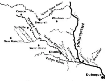
(4) J. Behmanesh et al.. J Fundam Appl Sci. 2015, 7(1), 91-102. 94. words, this study links the water management concept to the runoff control by using three different modeling techniques in modeling the rainfall-runoff process.. 2. MATERIALS AND METHODS 2.1. Description of study area In this study, modeling techniques were employed for the Turkey River watershed in order to model for the rainfall-runoff process. Turkey river length is 246Km which is a branch of Mississippi river. Turkey river watershed area is 4384 Km2. Figure (1) shows the situation of Turkey river. The data used in this study obtained from the web site of United State Geological Survey organization (USGS) in Spilliville station. The mentioned daily data have been recorded from 2011/10/6 to 2013/2/16. The statistical properties of rainfall-runoff for the Turkey River in the range of 6/10/2011 to 16/2/2013 have been shown in Table 1.. Fig.1. Watershed of Turkey River. Table 1 The estatistical properties of rainfall-runoff for the Turkey River in the range of 6/10/2011 to 16/2/2013 Daily Rainfall (mm/day) 490 1.4 46.7 0. Daily Runoff (cms) 490 1.8 25.08 0.26. Statistical characteristics The number of data Average Max Min.

(5) J. Behmanesh et al.. J Fundam Appl Sci. 2015, 7(1), 91-102. 95. 2.2. Back propagation artificial neural network Back Propagation Artificial Neural Networks (BPANN) include layers which have elements with parallel functions. Each of those elements is called a Neuron and data is processed within them. Each layer is different with the previous and the next layer but it is in connection with them. WIH and WHO indices are important which indicate the weight of the joints between the layers. Initial estimations will improve following the development of the model. As a result, the necessary correction value is determined in order to minimize the error. There are some advantages attributed to BPANNs such as adaptive learning, which means self-correction of the network, self-organization, which means that the neurons will adopt themselves to the new regulations and the respond to the input will change, immediate performance, which means that computations can be conducted in a parallel manner, error tolerance, which means the overall performance of the model remains unscathed if a small part faces an error, Grouping, which is the ability of categorizing the inputs in order to find an appropriate output, generalization, which is the ability of the model to generate a general rule by facing only a few species and expand the results to new inputs and finally the sustainability and flexibility of the technique. Two last abilities cause the technique to save the previous data and accept new inputs while saving time. In this study, Q-net software was employed to model the rainfall-runoff relationship in the Turkey River using ANN. Three hidden layers with three neurons and sigmoid function are used for each used model. Since the river flow rate depends upon pervious days data, modeling was conducted using present and pervious days data. Consequently ANN was created as dynamic network. 2.3. Adaptive Neuro Fuzzy Inference System (ANFIS) Fuzzy logic and fuzzy set theory have been widely used to simulate the ambiguity and uncertainty in various engineering problems. ANFIS techniques expands the quantity of the answers of the problem to a numerical category with range of 0 to 1 rather than a true/false answer. The governing rule of ANFIS is ‘if X is small, then Y is large’. This rule is applied to the neural network in order to enable the application of artificial networks in the model. The advantage of this model is its ability to explain the solution, while other models fail to provide an explain of the solution. The MATLAB software was used to model the river flow.

(6) J. Behmanesh et al.. J Fundam Appl Sci. 2015, 7(1), 91-102. 96. in ANFIS method. In modeling by ANFIS, 1000 epoch was used and input data were entered to model with similar weighing.. 2.4. Evaluation criteria In order to evaluate the used models, the statistical parameters as coefficient of determination (R2), Root Mean Square Error (RMSE) and Mean Absolute Error (MAE) were calculated. To calculate R2, RMSE and MAE, equations 1 to 3 were used respectively: 2   Qe  Qo  2 R  1   Qo  Qo .   Qe  Qo  RMSE  N. MAE . 1 N. | Q  Q e. o. (1). 2. |. (2). (3). where N is number of data and Qe and Qo stand for estimated and observed data respectively.. 2.5. Data collection The daily data in this research included the rainfall and the river flow rate which had been recorded in a period of 16 months. Two variables including rainfall runoff were employed to determine the river flow using lag-time methods. Table 2 shows the combination of input data. The subscripts t, t-1 and … indicate the input data corresponding to present time, one day ago and … respectively. For example M4 model states that there are five input data including Rt, Rt-1, Rt-2, Rt-3 and Qt-1 so that R and Q indicate runoff and flow rate respectively. Table 2: Combination of the inputs of different models Model output Input M1 Qt Rt Rt-1 M2 Qt Rt Rt-1 Rt-2 M3 Qt Rt Rt-1 Rt-2 Rt-3 M4 Qt Rt Rt-1 Rt-2 Rt-3 Qt-1 M5 Qt Rt Rt-1 Rt-2 Rt-3 Qt-1 Qt-2 M6 Qt Rt Rt-1 Rt-2 Rt-3 Qt-1 Qt-2 Qt-3.

(7) J. Behmanesh et al.. J Fundam Appl Sci. 2015, 7(1), 91-102. 97. 80% and 20% data were used in train and verification process. In order to create the regression relationship between rainfall and runoff for the Turkey river, the SPSS software was employed using mention input data in table 2. 3. RESULTS AND DISCUSSION 3.1. Numerical modeling Table 3 shows the statistical parameters for ANN model in train and verification stages. Table 3: Results of AAN model (Train: modeling with 80% of data. Test: modeling with 20% of data to test the Train model results) Models Train Test R2. MAE. RMSE. R2. MAE. RMSE. M1. 0.120 47.989 105.075 0.046 34.889 56.632. M2. 0.327 44.485. 87.026. 0.225 35.032 53.447. M3. 0.479 41.470. 69.346. 0.246 35.312 50.768. M4. 0.916 10.409. 14.382. 0.646 14.203 38.521. M5. 0.925 10.167. 7.022. 0.695 13.456 28.211. M6. 0.913 10.203. 5.023. 0.668 13.757 35.558. As it can be seen from table 3, the M5 model has the best results in the comparison of other employed models. In mentioned model RMSE and MAE have the lowest value and R2 has the highest amount. The statistical results by using ANFIS method has been presented in table 4.. Table 4: Results of ANFIS Model (Train: modeling with 80% of data. Test: modeling with 20% of data to test the Train model results) Train Test Models R2 MAE RMSE R2 MAE RMSE M1. 0.186 47.142 103.053 0.1146 34.4972 51.245. M2. 0.415 42.183. 77.562. 0.2511 34.4772 51.710. M3. 0.627 35.409. 61.897. 0.3046 34.9765 53.754. M4. 0.985. 5.062. 12.097. 0.6143 15.6610 32.710. M5. 0.994. 3.919. 7.425. 0.7727 11.7010 24.427. M6. 0.998. 5.209. 4.342. 0.5818 14.6903 35.495.

(8) J. Behmanesh et al.. J Fundam Appl Sci. 2015, 7(1), 91-102. 98. As it can also be seen from table 4, the ANFIS model has the best results and M5 model is presented as the best model. RMSE values in ANN and ANFIS models were obtained 28.211m3/sec and 4.428m3/sec respectively in the verification stage by M5 models. Having the best results of M5 model Shows that the present flow rate has the best fit with Rt, Rt-1, Rt-2, Rt-3, Qt-1 and Qt-2. In fact, up to M3 models, the models accurate is not acceptable due to using only rainfall as input data but for models from M4 to M6, the model accuracy was improved because of using the flow rate data in previous days. The comparison of M5 and M6 models shows that M5 has better result than M6 model. This result can be explained from the concentration time consideration which can be about two days. Figure 2 shows the variations of determination coefficient for ANN and ANFIS models.. Fig.2. Comparison of the results of application of two techniques It can be seen from Figure 2 that the ANFIS model has better results than ANN models. Figures 3 and 4 show the results of M5 model in verification stage for ANN and ANFIS modeling respectively. Figures 3 and 4 also show that ANFIS model present better results than ANN model. Figure 5 shows the comparison of observed and simulated data..

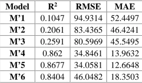
(9) J. Behmanesh et al.. J Fundam Appl Sci. 2015, 7(1), 91-102. 99. Fig.3. Results of M5 model in verification stage for ANN modeling. Fig.4. Results of M5 model in verification stage for ANFIS modeling. Fig.5. Comparison of observed and simulated data. 3.2. Regression modeling Equations 4 to 9 show the results of linear regression using different input data. These equations were obtained by using the SPSS software. The released statistical parameters due to regression analysis have been showed in table 5. M’1: f(Qt)=52.599Rt+165.183Rt-1+56.380. (4). M’2: f(Qt)=56.476Rt+138.906Rt-1+175.346Rt-2+44.782. (5).

(10) J. Behmanesh et al. 100. J Fundam Appl Sci. 2015, 7(1), 91-102. M’3: f(Qt)=55.816 Rt+139.739Rt-1+164.545Rt-2+123.619Rt-3+38.507. (6). M’4: f(Qt)=20.531 Rt+91.905 Rt-1+40.462Rt-2-32.399Rt-3+0.866Qt-1+1.313 (7) M’5: f(Qt)=19.572 Rt+89.193 Rt-1+24.538Rt-2-35.251Rt-3+1.073Qt-1-0.194Qt-2+2.917 (8) M’6: f(Qt)=20.363 Rt+89.256 Rt-1+23.381Rt-2-16.645Rt-3+1.122Qt-1-0.477Qt-2+0.252Qt-3+0.820. (9). Table 5 statistical parameters for regression analysis Model M’1 M’2 M’3 M’4 M’5 M’6. R2 0.1047 0.2061 0.2591 0.862 0.8677 0.8404. RMSE 94.9314 83.4365 80.5969 34.8461 34.0581 46.0482. MAE 52.4497 46.4241 45.5495 13.9632 12.6648 18.3503. It’s clear from Table 5 that M’5 has the best results. Therefore, to predict the flow rate in Turkey river, the M’5 model can be selected. Figure 6 shows the comparison of Regression modeling with observed data.. Fig.6. Comparison of Regression modeling with observed data.

(11) J. Behmanesh et al. 101. J Fundam Appl Sci. 2015, 7(1), 91-102. 4. CONCLUSIONS In this research the relationship between rainfall and runoff in Turkey River was modeled using ANN, ANFIS and linear regression. The result of this study showed that the ANFIS model had the best results. M5 model among other models was presented as a selected model which was using four rainfalls and two flow rates as input data. Comparing M5 and M6 models in ANFIS modeling showed that the watershed concentration time for studied area was about two days. This conclusion can be obtained from the results obtained from M5 models.. 5. REFERENCES [1] Hundecha, Y. Bardossy, A. Theisen, HW. 2001. Development of a fuzzy logic-based rainfall-runoff model. Hydrologic Sciences Journal 46(3): 363–376. [2] Babovic, V. Keijzer, M. Rainfall runoff modeling based on genetic programming. Water Resources Research Nordic Hydrology, 33 (5), 2002,33 1-346 [3] Agarwal, A. Singh, RD. 2004. Runoff modeling through back propagation artificial neural network with variable rainfall-runoff data. Water Resources Management,18: 285–300. [4] Nayak, PC. Sudheer, KP. Rangan, DM, Ramasastri, KS. 2004. A neuro-fuzzy computing technique for modeling hydrological time series. Journal of Hydrology. Volume 291, Issues 1–2, 31 May 2004, Pages 52–66. [5] Ahmad, S. Simonovic, P. 2005. An artificial neural network model for generating hydrograph from hydro-meteorological parametrs. Journal of hydrology .vol, 315: 236-251. [7] Kalteh, A M. 2008. Rainfall-runoff modeling using artificial neural networks (ANNs): modeling and nderstanding. Caspian J. Env. Sci. Vol. 6 No.1 pp.53-58. [9] Lohani, L K. 2010, Hydrological processes, Wiley Online Library, 25, 175–193 2011. [10] Mukerji, A. Chatterjee, C. Raghuwanshi, N. 2009. Flood forecasting using ANN, neuro-fuzzy, and neuro-GA models. J. Hydrol. Eng., 14(6), 647–652..

(12) J. Behmanesh et al. 102. J Fundam Appl Sci. 2015, 7(1), 91-102. [11] Kumar, P. Kumar, D. 2012. Rainfall-runoff modeling of a watershed. Civil and Environmental Research ,Vol 2, No.2, 2012. [12] Taheri, H. Ghafouri, MR. Bagheri, S. Saghafian, B. Nasseri, M. 2012. Comparison between active learning method and support vector machine for runoff modeling. J. Hydrol. Hydromech, 60, 2012, 1, 16-32 [13] Kakaei Lafdani, E. Moghaddam Nia, A. Pahlavanravi, A. Ahmadi, A. Jajarmizadeh, M. 2013. Daily Rainfall-Runoff prediction and simulation using ANN, ANFIS and conceptual hydrological MIKE11/NAM models. International Journal of Engineering & Technology Sciences (IJETS) 1 (1): 32-50, 2013. How to cite this article Behmanesh J, Ayashm S. Rainfall-runoff modeling in the turkey river using numerical and regression methods. J Fundam Appl Sci. 2015, 7(1), 91-102..

(13)