THESIS PRESENTED TO
ÉCOLE DE TECHNOLOGIE SUPÉRIEURE
IN PARTIAL FULFILLMENT OF THE REQUIREMENTS FOR A MASTER’S DEGREE IN ELECTRICAL ENGINEERING
M. A. Sc.
BY
Nasim OLIAZADEH
DEVELOPMENT AND PERFORMANCE ANALYSIS OF AN ATTITUDE
DETERMINATION SYSTEM USING MULTIPLE GPS RECEIVER CONFIGURATION
MONTREAL, MARCH 9th 2016
© Copyright
Reproduction, saving or sharing of the content of this document, in whole or in part, is prohibited. A reader who wishes to print this document or save it on any medium must first obtain the author’s permission.
BY THE FOLLOWING BOARD OF EXAMINERS
Prof. René Jr. Landry, Thesis Supervisor
Department of Electrical Engineering at École de technologie supérieure
Prof. Rachid Aissaoui, Chair, Board of Examiners
Department of Automated manufacturing Engineering at École de technologie supérieure
Prof.Christian Gargour, Member of the jury
Department of Electrical Engineering at École de technologie supérieure
Mr.Eric Gagnon, External Evaluator
Defence Scientist, Valcartier Research Centre
THIS THESIS WAS PRESENTED AND DEFENDED
IN THE PRESENCE OF A BOARD OF EXAMINERS AND THE PUBLIC FEBRUARY 25 th 2016
Foremost, I would like to express my sincere gratitude to my advisor Prof. René Jr. Landry to give me the opportunity to work on this project and for the continuous support during my master study, and also for his patience and motivation.
My sincere thanks also go to Dr. Omar Yeste Ojeda and Dr.Mohammad Ali Goudarzi for their insightful comments and guidance during my master. I would like also to thank the professional researcher of LASSENA, Adrien Mixte for assisting me to acquire real data and for his guidance during my master.
And an especial thanks to our industrial partner, Numerica.Inc and Fonds de recherche du Québec – Nature et technologies (FRQNT) for funding this project, without whom this work was not possible.
Last but definitely not least, I would like to thank my family, my dear sister and my brother in law with their continuous love and support during my master, where I was far from my hometown. Especial thanks goes to my wonderful mom and dad for their unconditional love and support.
DEVELOPMENT AND PERFORMANCE ANALYSIS OF AN ATTITUDE DETERMINATION SYSTEM USING MULTIPLE GPS RECEIVER
CONFIGURATION
Nasim OLIAZADEH
SUMMARY
Up to now, attitude determination systems are using high cost GNSS receivers or the combination of both GNSS receivers and other sensors mainly Inertial Navigation Systems. The problem is, the INS systems are either high cost or they suffer from increasing drift over the time. Nowadays the cost, weight, flexibility of use and small aperture of the attitude determination system are the main concerns. The main objective of this thesis is to get 3-D attitude angles by designing a low cost attitude determination system which processes raw GPS measurements.
To make this goal happen, we designed a recursive least-squares algorithm by combining both code and carrier phase measurements and fixing the ambiguity parameters with least-squares ambiguity decorrelation adjustment method. In order to achieve robust attitude estimation, we used singular value decomposition method that is an estimator for Wahba’s loss function. Then, in order to analyze the performance of the designed ADS, we prepared different test cases in both simulation and real data sets. The baseline is qualified as an ultra-short baseline and the only measurement used is the GPS L1 signal.
By using a GPS simulator and two u-blox LEA-6T receivers synchronized together and without the presence of multipath, an accuracy of 0.03° and 0.06° for heading and elevation has been achieved. For an overall, even though LAMBDA method improved the solution accuracy in all test cases, in the presence of the multipath error, it does not converge to the right solution. Synchronizing all clock receivers by hardware and avoid the multipath are the main limitations of this work. Such a light weight and low cost system with the accuracy of millidegree in the attitude angles can be used in a wide range of applications consisting civil and military applications.
DÉVELOPPEMENT ET ANALYSE DES PERFORMANCES D'UN SYSTÈME DE DÉTERMINATION DE L'ATTITUDE D'UN MOBILE UTILISANT PLUSIEURS
RÉCEPTEURS GPS
Nasim OLIAZADEH
RÉSUMÉ
Jusqu'à présent, les systèmes de détermination d'attitude utilisent des récepteurs GNSS haut de gamme ou une combinaison de récepteurs GNSS avec d'autres capteurs tels que les centrales inertielles (INS). Cependant, les systèmes INS ont un coût plus élevé ou alors ils souffrent d’une dérive importante au cours du temps. De nos jours, le coût, la taille, le poids et la flexibilité d’utilisation sont des éléments importants pour les industriels. L’objectif principal de cette thèse est d’obtenir l’attitude en 3D d’un mobile grâce à la conception d’un système de détermination d’attitude à faible coût basé sur l’utilisation de mesures GNSS brutes.
Afin de répondre à cet objectif, nous avons conçu un algorithme récursif utilisant la méthode des moindres carrés en combinant les mesures de code et de phase de la porteuse. On peut ainsi fixer les paramètres d’ambigüité avec la méthode d’ajustement de la décorrélation d’ambiguïté des moindres carrés. Afin de parvenir à une estimation robuste de l’attitude, nous avons utilisé la méthode de décomposition de valeur singulière qui est un estimateur de la fonction de perte de Wahba. Puis, afin d'analyser la performance des ADS conçus, nous avons préparé différents cas de test à la fois en simulation et avec des données réelles. Le vecteur de baseline est de faible distance et les mesures utilisées proviennent du signal GPS L1.
En utilisant un simulateur de GPS et deux récepteurs u-blox LEA-6T, nous avons obtenu une précision de 0,03° et de 0,06° respectivement pour l’angle du cap et pour l’élévation, ceci sans la présence de trajets multiples. Dans l’ensemble, la méthode LAMBDA permet d’améliorer la précision de la solution, cependant en présente d’erreurs de multi-trajets, la solution ne converge pas. L’absence de synchronisation des différentes horloges des récepteurs ainsi que le multi-trajet a limité les performances des algorithmes. Malgré tout, le faible poids ainsi que le faible coût du système, fonctionnant avec une précision d’attitude en millidegree, peut être utilisé dans de nombreuses applications dans le domaine civil et militaire.
TABLE OF CONTENTS Page CHAPTER 1 INTRODUCTION ...1 1.1 Research problems ...3 1.2 Research objectives ...4 1.3 Research methodology ...4 1.4 Contributions...6 CHAPTER 2 GPS OVERVIEW ...9 2.1 GPS segments ...9
2.2 GPS signal and data characteristics ...11
2.2.1 Navigation data structure ... 13
2.3 Mathematical modelling of GPS measurements and errors ...15
2.3.1 GPS measurement and associated errors ... 15
2.3.1.1 Code measurement and associated errors ... 15
2.3.1.2 Carrier phase measurement ... 16
2.3.1.3 Doppler ... 17
2.3.2 Differential GPS... 18
2.3.2.1 Single difference ... 18
2.3.2.2 Double difference ... 20
2.3.2.3 Triple difference ... 21
2.3.3 Other residual errors ... 21
2.3.3.1 Phase center variation ... 21
2.3.3.2 Multipath ... 22
2.4 Important parameters in satellite geometry ...25
2.4.1 Elevation and azimuth ... 25
2.4.2 Quality metrics of GNSS constellation ... 26
2.5 Important references for GNSS navigation ...28
2.5.1 Earth centred earth fixed reference frame ... 29
2.5.2 Local frame ... 29
2.5.3 Body frame and Euler angles ... 30
2.6 Rotation Matrix ...31
CHAPTER 3 LITERATURE REVIEW ...33
3.1 Methods of GPS ambiguity resolution ...33
3.1.1 Ambiguity function method ... 35
3.1.2 Least-squares ambiguity search technique ... 36
3.1.3 Fast ambiguity resolution approach ... 37
3.1.4 Fast ambiguity search filter ... 37
3.1.5 Least-squares ambiguity decorrelation adjustment ... 38
3.1.6 Summary ... 41
3.2 Attitude determination methods ...42
3.2.2 Baseline method for attitude determination ... 45
3.2.2.1 Quaternion method for attitude determination ... 47
3.2.2.2 QUEST method for attitude determination ... 49
3.2.2.3 SVD method for attitude determination ... 50
3.2.2.4 FOAM method for attitude determination ... 52
3.2.2.5 ESOQ method for attitude determination ... 52
3.2.2.6 ESOQ2 method for attitude determination ... 53
3.2.3 Summary of attitude determination algorithms ... 54
3.3 GPS and GLONASS integration ...55
3.4 Conclusion ...62
CHAPTER 4 ADS ALGORITHM DESIGN ...63
4.1 Data selection ...64
4.2 Single point positioning algorithm with pseudorange ...65
4.3 Presentation of designed baseline estimation algorithm ...68
4.3.1 General optimization problem ... 68
4.3.1.1 RLS mathematical procedure ... 70
4.3.2 Ambiguity resolution using LAMBDA method ... 77
4.3.3 Check the constraint ... 78
4.4 Attitude determination using the SVD method ...78
CHAPTER 5 IMPLEMENTATION AND ANALYSIS OF THE RESULTS ...81
5.1 ADS performance analysis, test case 1 ...81
5.2 ADS performance analysis, test case 2 ...92
5.3 ADS performance analysis, test case 3 ...99
5.4 ADS performance analysis, test case 4 ...103
CHAPTER 6 CONCLUSION AND FUTURE WORKS ...113
6.1 Conclusion ...113
6.2 Future works ...115
LIST OF TABLES
Page
Table 3.1 Attitude determination method comparison ...55 Table 3.2 Mathematical models for combined GPS and GLONASS positioning ...60 Table 5.1 Variance comparison in test case 1 ...85 Table 5.2 Variance comparison for Euler angles estimation ...88 Table 5.3 A summary of different test cases ...111
LIST OF FIGURES
Page
Figure 1.1 Geometry of the defined project ...2
Figure 2.1 Control segment ...10
Figure 2.2 GPS signals generation ...12
Figure 2.3 BPSK modulation with C/A code and navigation message ...13
Figure 2.4 GPS navigation data structure ...14
Figure 2.5 Doppler effect ...17
Figure 2.6 Multipath effect ...23
Figure 2.7 Azimuth and elevation angles ...26
Figure 2.8 Effect of signal geometry on the position accuracy ...26
Figure 2.9 Satellite geometry ...27
Figure 2.10 ECEF frame axis ...29
Figure 2.11 Local frame, ENU ...30
Figure 2.12 Body frame ...31
Figure 3.1 GPS phase difference geometry ...44
Figure 3.2 Baseline vectors of our defined project ...45
Figure 4.1 Global ADS algorithm flowchart ...63
Figure 4.2 Master antenna position error by using SPP algorithm ...67
Figure 4.3 Geometry for two receivers and one satellite ...70
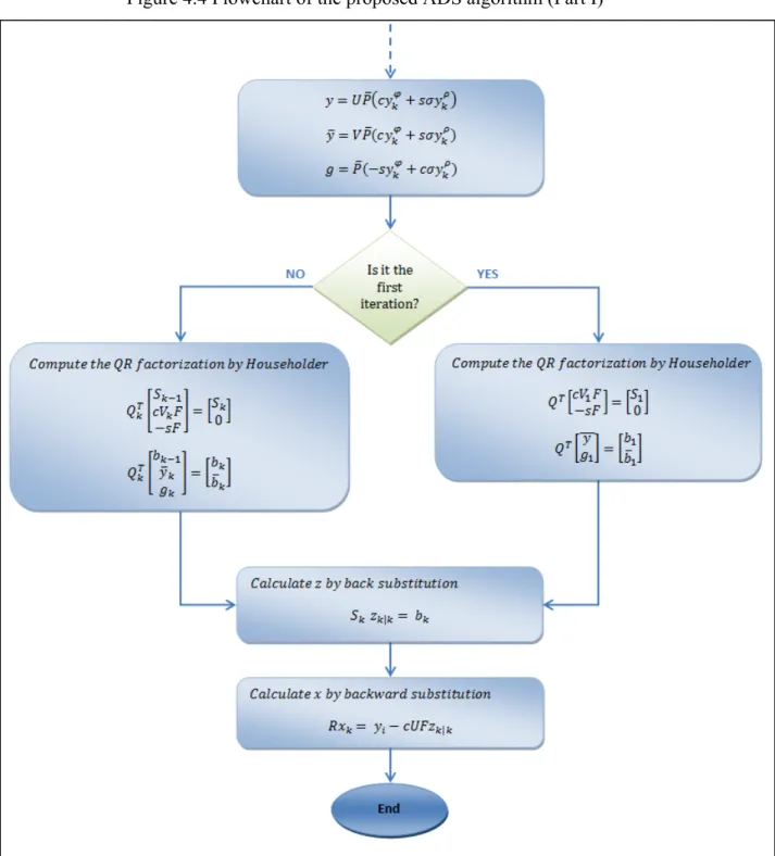
Figure 4.4 Flowchart of the proposed ADS algorithm (Part I) ...76
Figure 4.5 Flowchart of the proposed ADS algorithm (Part II) ...76
Figure 5.2 Baseline estimation error before convergence in test case 1 ...83
Figure 5.3 Baseline estimation error after convergence test case 1 ...84
Figure 5.4 Baseline estimation variance ...85
Figure 5.5 Euler angles error before convergence in test case 1 ...86
Figure 5.6 Euler angles error after convergence in test case 1 ...87
Figure 5.7 Euler angles estimation variance ...87
Figure 5.8 Baseline estimation error comparison before convergence comparison in test case 1 ...89
Figure 5.9 Baseline estimation error comparison after convergence in test case 1 ....89
Figure 5.10 Pitch estimation error comparison before convergence in test case 1...90
Figure 5.11 Pitch estimation error comparison after convergence in test case 1 ...91
Figure 5.12 Comparison between designed ADS and previous works in literature test case 1 ...91
Figure 5.13 Estimated baseline components, test case 2 ...93
Figure 5.14 Relation between the estimation error, GDOP and the ambiguities in test case 2 ...94
Figure 5.15 Heading estimation intest case 2 ...95
Figure 5.16 Elevation estimation in test case 2 ...95
Figure 5.17 Heading estimation and the detected outliers in test case 2 ...97
Figure 5.18 Elevation estimation and the detected outliers in test case 2 ...97
Figure 5.19 The least-squares moving ramp passed through the heading estimation ..98
Figure 5.20 The least-squares moving ramp passed through the elevation estimation 99 Figure 5.21 Data record configuration with two u-blox LEA-6T and two G5Ant-4AT1 ...100
Figure 5.22 Baseline estimation in test case 3 ...101
Figure 5.23 Relation between the estimation error, GDOP and the ambiguities in test case 3 ...101
Figure 5.24 Estimation error in test case 3 ...102 Figure 5.25 Data record configuration in test case 3 ...104 Figure 5.26 Baseline 1 estimation in test case 4 ...105 Figure 5.27 Relation between the estimation error, GDOP and the ambiguities
in test case 4, baseline 1 ...106 Figure 5.28 Baseline 2 estimation in test case 4 ...107 Figure 5.29 Relation between the estimation error, GDOP and the ambiguities
in test case 4, baseline 2 ...108 Figure 5.30 Baseline 3 estimation in test case 4 ...108 Figure 5.31 Relation between the estimation error, GDOP and the ambiguities
in test case 4, baseline 3 ...109 Figure 5.32 Attitude angles error versus baseline estimation error ...110 Figure 6.1 Global ADS flowchart ...114
LIST OF ABREVIATIONS, INITIALS AND ACRONYMS
AFM Ambiguity Function Method
AFSCN Air Force Satellite Control Network
C-LAMBDA Constrained Least-Square AMBiguity Decorrelation Adjustment BPSK Binary Phase Shift Keying
CDMA Code Division Multiple Access
CS Control Segment
DD Double Difference
DGPS Differential GPS
DOP Dilution Of Precision E East ECEF Earth Centered Earth Fixed EKF Extended Kalman Filter
FARA Fast Ambiguity Resolution Approach FASF Fast Ambiguity Search Filter
FDMA Frequency Division Multiple Access
FIR Finite Impulse Response
FOAM Fast Optimal Attitude Matrix
FOC Full-Operational-Capability
FRQNT Fonds de Recherche du Québec – Nature et Technologies
FT Fourier Transform
GDOP Geometry Dilution Of Precision GLONASS GLObal NAvigation Satellite System
GLONASST GLONASS Time
GNSS Global Navigation Satellite System GPS Global Positioning System
GPST GPS Time
HDOP Horizontal Dilution Of Precision
IID Identically Independently Distributed
ILS Integer Least-Squares
IMU Inertial Measurement Unit INS Inertial Navigation System
LAMBDA Least-squares AMBiguity Decorrelation Adjustment
LOS Line Of Sight
LSAST Least-Squares Ambiguity Search Technique MILS Mixed Integer Least -Squares
N North
NGA National Geospatial-intelligence Agency
OTF On The Fly
PCV Phase Center Variation
PDOP Position Dilution Of Precision PNT Positioning, Navigation, and Timing PZ90 Parametry Zemli 1990
OUEST QUaternion ESTimator
RINEX Receiver INdependent EXchange format
RLS Recursive Least-Squares
RMSE Root Mean Square Error
SBAS Satellite Based Augmentation System
SD Single Difference
SNR Signal to Noise Ratio SPP Single Point Positioning
SS Space Segment
SVD Singular Value Decomposition
TD Triple Difference
US User Segment
USAF United State Air Force USG United State Government
UTC Universal Time Coordinated
UTC-SU Universal Time Coordinated, Soviet Union standard WGS84 World Geodetic System 84
CHAPTER 1 INTRODUCTION
A simple definition of navigation can be described as the best possible estimate of the position, velocity, and attitude of a moving object. Historically, navigation has been associated with guiding ships through the desired route using compass. However, nowadays navigation is an extensive field which can be found everywhere from cell phones and wristwatches to aviation, mapping, surveying and search and rescue. The most effective way to achieve a robust and consistent navigation system is through the technology of the Global Positioning System (GPS). The GPS offers an accurate, free, continues, weather-proof, and globally available satellite-based navigation services, which makes it a seamless tool to satisfy many of needs for navigation purposes. The accurate determination of position, velocity, acceleration, and time, in both relative and absolute sense, construct the main applications of this technology.
Among recent applications of such a system is to determine the orientation of the object’s body frame with respect to a known reference frame. This is called attitude determination. By using high-cost receivers and antennas, as well as high-frequency signal transmission rates (e.g., P-code), this technology provides highly precise measurements, and has been used in high sensitivity applications such as military applications. Nevertheless, these systems are commonly expensive and large in size and the use of such systems may be restricted by governments. For example, the P-code is only available for the USA armed forces.
The overall objective of this thesis is to provide an inexpensive and light-weight alternative to conventional attitude determination systems using the GPS technology. In particular, we are interested in low-cost and light-weight receivers and antennas in a compact configuration with civil frequency ranges (i.e. L1 frequency).
This work tries to answer the following questions: What are the limitations of such a system? How much precision can be obtained? Is it possible to replace those expensive and heavy systems with such a low-cost and light-weight system? Such an attitude determination system is an opening window to a wide range of applications from smartphones in civil applications to military purposes and precise applications.
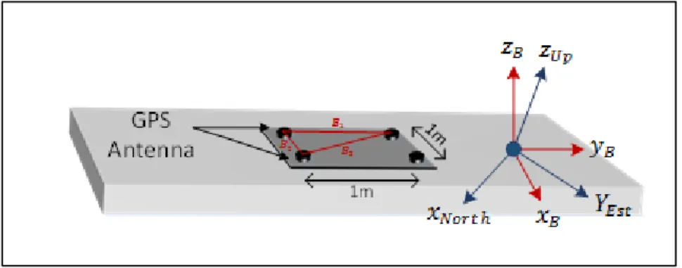
Our industrial partner Numerica.Inc searches for a low-cost and light weight system to measure the position of an object1. This object is located within about 1 km distance from the observer and it needs to be located within an error of 1m. Such a system needs two measuring systems, one of them is to measure the distance between the object and the observer, and the other one to measure the 3-D attitude of the observer pointing system aiming the object. The focus of this work is to determine the attitude of the observer pointing system with precision of about 0.05° for the yaw, pitch, and roll angles so the object can be located within 1m error, Figure 1.1.
1m
1 km
0.05°
Figure 1.1 Geometry of the defined project
This thesis has the following structure. This chapter present an overview of the research problem, objectives and methodology. Chapter 2 presents an overview of GPS constellation and signals, GPS segments and its data characteristics. This chapter also outlines the
1 This project is funded by Fonds de Recherche du Québec – Nature et Technologies (FRQNT) and our
mathematical modelling of GPS measurements and their associated errors as well as error cancelling techniques.
Chapter 3 provides a detailed literature review on the most challenging problems of the project, namely ambiguity resolution and attitude determination methods. Chapter 4 is dedicated to the proposed methodology for the Attitude Determination System (ADS), its mathematical procedure and algorithm. The details of the proposed ADS developments are explained extensively in this chapter.
Chapter 5 is dedicated to result presentation, comparison and discussion. In order to analyse the performance of the ADS, we designed different test cases with different configurations, receivers, antennas and record locations. Some concluding remarks as well as some future works to improve the proposed ADS are presented in chapter 6.
1.1 Research problems
The research problems of this project can be expressed as follows:
1. GPS has two main types of observables: pseudorange measurements which are the range between the receiver and the satellite, and carrier phase measurements which are measured as the phase difference of received signal and the replica in the receiver. In order to obtain a precise solution for attitude determination, using phase measurement that is about 100 times more precise than the code measurement is necessary. The main problem of using this measurement is its ambiguity resolution that needs to be solved and fixed. Ambiguity resolution will be explained in details in the next chapter;
2. A computational time reduction strategy needs to be applied in order to be able to use the designed ADS system real time;
3. To increase accuracy and availability of GNSS satellites, it is advantageous to incorporate other GNSS signals into the ADS algorithm. This needs to overcome the difference between GNSS constellation which needs to be studied.
In this research, the main research problematic is consist of solving ambiguity parameters of several low-cost GPS receivers which are synchronized together and to develop an attitude determination algorithm in order to compute the 3-D attitude angles precisely. The raw measurements are limited to GPS L1 and can be affected by noises as well as errors namely multipath error. Those effects will need to be processed according to the state-of-the-art processing techniques.
1.2 Research objectives
The main objective of this thesis is to determine the 3D attitude angles of a moving platform using four low-cost GPS receivers attached to the platform with an attitude resolution better than 50m degrees. This resolution is necessary to secure the localization of an object at 1km within an error of 1 meter. In accordance with and to fulfill the main objective of this research, there are 4 defined specific objectives. The first one is to fix the ambiguity parameters as an integer. The second one is to synchronize several receivers by hardware or software algorithm. The third one is to investigate the processing load of the designed system in order to use the developed attitude determination system in real-time applications. The last objective is to investigate theoretically how to incorporate measurements of the Global Navigation Satellite System (GLONASS) of the Russian federation into the system.
1.3 Research methodology
In order to fulfil the research objectives, we conduct our work in four algorithm modules which are:
1. Data selection: An algorithm is designed to filter the data based on satellites
of compromising between number of satellites and duration of satellite visibility depends on the user’s choice in order to get a proper period of data for analysis;
2. Single point positioning: We calculate the master antenna position with Single Point
Positioning (SPP) algorithm. This algorithm uses only pseudorange measurements in order to have an approximate position of the master antenna. In this module, we also calculate satellite positions as well as calculating receiver and satellite’s clock errors;
3. Baseline estimation: In order to estimate the baseline vectors, a Recursive
Least-Squares (RLS) method is designed and developed by combining both code and carrier measurements. By taking advantage of the structure of the problem, we try to decrease the computational cost of the algorithm as well as preserving the accuracy. All the three aspects of computer implementation, namely numerical reliability, computational, and storage efficiency have been considered in this method. We also use the configuration information, baseline length, and fix the ambiguity with Least-squares AMBiguity Decorrelation Adjustment (LAMBDA) method;
4. Attitude determination: In this module we developed Singular Value
Decomposition (SVD) method which is an estimator for Wahba’s loss function. This algorithm does not need a-priori information for dynamic applications.
Along with the mentioned methodology for the designed algorithm, the research methodology is as follows:
1. Development a complete attitude determination system consisting 4 main mentioned modules of the algorithm in Matlab. The inputs are GPS L1 raw measurements and the outputs are the 3-D attitude angles;
2. Test the complete designed system using simulated data (in Matlab and with GPS simulator). This step is designed to validate the developed algorithms;
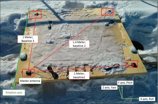
3. Build a platform and mounting four low-cost receivers and antennas to acquire sufficient GPS raw measurements. In order to compare the results, two pairs of low-cost receivers and high-low-cost antennas are mounted on the platform as well;
4. Analyze the performance of the ADS algorithm using real GPS L1 measurements for all the test cases.
Furthermore, a detailed theoretical research is done to incorporate GLONASS measurements into this system in order to achieve much precise and reliable system even without a suitable visibility for GPS constellation.
1.4 Contributions
The contributions of this research can be summarized as follows:
1. Designing an ADS algorithm and system combining four main modules:
to read, to filter and to synchronize the incoming raw measurements from 4 GPS L1 receivers. The input of this module is raw measurements from 4 GPS L1 receivers and the outputs are four set of filtered data based on the chosen criteria by the user, which are synchronized together in ms precision. The user can choose the analysis duration, the minimum used satellites, minimum
⁄ and the mask angle;
to estimate the position of GPS satellites using the SPP algorithm proposed by (Borre, 2003) and to compute the best geolocation position of the master antenna. The input of this module is the filtered data from previous step and the output is satellite positions and master antenna position;
to compute precise baseline vectors by the RLS algorithm. By having the master antenna position and satellite position, now we can compute the baseline vectors;
to compute precise Euler angles using the SVD method. The input of this module is 3 baseline vectors and the output is 3-D attitude angles.
2. Combining the RLS algorithm with the LAMBDA method according to (Joosten, 2001) in order to fix the float solution. Constrain the solution by using the prior configuration information. In this work we used baseline length to constrain the baseline estimation solution.
This research allows the publication of the following conference paper:
Oliazadeh, Nasim; Landry, Rene Jr; Yeste-Ojeda, Omar A; Gagnon, Eric and Wong, Franklin 2015. «GPS-based attitude determination using RLS and LAMBDA methods». In
Localization and GNSS (ICL-GNSS), 2015 International Conference on. p. 1-7. IEEE. doi:
CHAPTER 2 GPS OVERVIEW
In this chapter, we present an overview of GPS and navigation principals in order to give the reader a better understanding of the rest of thesis.
In the first section, we present a brief review on GPS constellation and segments. Then a comprehensive introduction on GPS measurements, common techniques and errors will be presented. Afterwards, we go through the most commonly used navigation frames and transformation matrices followed by a discussion about the satellite geometry in space and its impact on the solution accuracy.
2.1 GPS segments
Navstar Global Positioning System known as GPS, owned by the United States Government (USG) and operated by the United States Air Force (USAF), is the earliest and the most accurate space-based radio-navigation system of the world. This project, which has been started in 1973 and completed in 1994, provides accurate Positioning, Navigation, and Timing (PNT) 24 hours a day, in all weather and all over the world. GPS consists of three main segments: Space, Control and User segments.
The Space Segment:
The Space Segment (SS) consists of six orbital planes at an altitude of about 20,200 km above the earth's surface at an inclination angle of 55° with respect to the equatorial plane.
Each orbit has four equally-spaced slots for satellites, which is covered by at least one operational satellite all the time. For global coverage, USAF ensures availability of at least 24 satellites for 95% of the time. With this arrangement we always have at least 4 visible satellites, which is the minimum required number of satellites to calculate 3D position and time. GPS satellites carry atomic clocks with nanosecond accuracy and broadcast continues
radio frequency signals on the two carrier frequencies of L1 (1575.42 MHz) and L2 (1227.6 MHz).
The Control Segment:
The Control Segment (CS) is a ground-based global network to track and monitor GPS satellites consisting two master control stations, 16 monitoring stations including six from the Air Force and 10 from the National Geospatial-Intelligence Agency (NGA), 4 ground antennas and 8 Air Force Satellite Control Network (AFSCN).
Figure 2.1 Control segment Taken from Force (2015)
The monitoring stations collect data from each visible satellite and send them to the master control stations. The master control stations are responsible for computing extremely precise satellite orbits and send them, as an updated navigation massages, to the ground antennas. Then the ground antennas send updated navigation massage to each visible satellite. Finally in order to increase tracking robustness, the control segment is tracked by eight AFSCN remote tracking stations.
The User Segment:
User Segment (US) consists of all GPS receivers which receive and process GPS signals in order to calculate position and time.
2.2 GPS signal and data characteristics
The GPS signals are transmitted on two radio frequencies, L1 and L2 in L band. L1 and L2 are both derived from a common frequency called :
= 10.23 (2.1)
= 150 = 1575.42 MHz (2.2)
= 120 = 1227.60 MHz (2.3)
Each of these signals is consist of three parts:
• carrier: The carrier wave with and frequency;
• navigation message: This message is about satellite orbits and clock errors, which
are uploaded from the ground base control segment with 50 bps rate;
• spreading sequence: Each satellite has two unique spreading sequences. The first
one is Coarse Acquisition (C/A) code with 1.023 MHz frequency, and encrypted Precision (P(Y)) code with 10.23 MHz frequency. The C/A code is only modulated on L1 frequency while P(Y) is modulated on both L1 and L2.
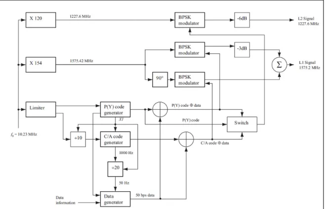
Figure 2.2 GPS signals generation Adapted from Benedetto et al. (2013)
Figure 2.2 is a detailed description of signal generation. At the left the main clock is supplied to three blocks which generate , and to the limiter to stabilize the clock signal. At the very bottom, the data generator generates the navigation data that is synchronized with code generators by X1 supplied by P(Y) generator. Afterwards, the generated codes through an exclusive OR operation, are combined with the navigation data. The resulted signals are modulated onto the carrier signal by Binary Phase Shift Keying (BPSK) method and with 90°
shift between two codes. As summary, the transmitted signal from satellite can be described as follows:
( ) = 2 ( )⨁ ( ) cos(2 )
(2.4)
+ 2 ( )⨁ ( ) sin(2 )
where , , and are the powers of the signals, ( ) is the C/A code of satellite , and ( ) is the navigation message.
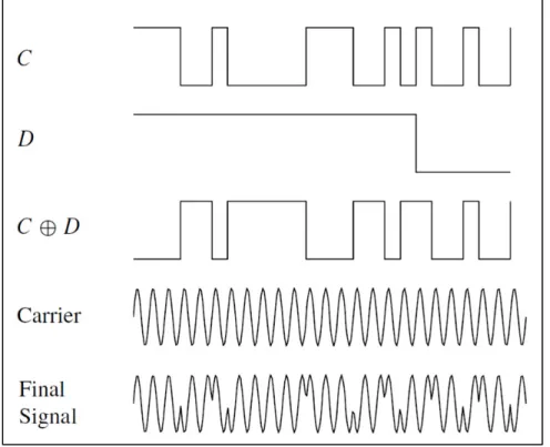
Figure 2.3 BPSK modulation with C/A code and navigation message Adapted from Benedetto et al. (2013)
Figure 2.3 shows the final signal modulation with BPSK after C/A code and navigation addition. Phase is shifted by 180° when the chip changes.
2.2.1 Navigation data structure
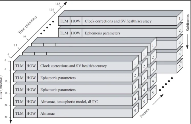
Navigation data with 50 bps rate is a 1500 bit-long frame which is consists of 5 subframes and each 300 bits long. Each subframe contains 10 words and each of them has 30 bits length. By 50 bps rate, a transmitted subframe lasts 6 s, one frame lasts 30 s and one entire navigation massage lasts for 12.5 minutes, Figure 2.4.
Figure 2.4 GPS navigation data structure Adapted from Benedetto et al. (2013)
Each subframe contains 10 words which always starts with two words, the telemetry and
handover word followed by 5 subframes as follows:
• telemetry (TML) is the first word that is repeated every 6 s. TML contains 8-bit
preamble and 16 reserved bit and parity which are used for frame synchronization;
• handover (HOW) contains of 17-bit of time of week and antispoofing flag followed
by the subframe ID;
• satellite clock and health is used to calculate navigation message transmission time
and satellite information is used to inform whether the data can be trusted or not;
• support data subframe is contained almanac, ionospheric model, UTC parameters,
etc. The almanac data is the ephemeris data with reduced precision. Each satellite send almanac data for all GPS satellites while each satellite only transmits ephemeris data for itself.
2.3 Mathematical modelling of GPS measurements and errors
This section presents the GPS measurements and their mathematical modelling briefly. Then three kinds of differential techniques and their equations will be presented. In the last section, the most common errors in these measurements will be discussed.
2.3.1 GPS measurement and associated errors
Most of the GPS receivers provide three types of measurements: Pseudorange, Carrier phase, and Doppler. These measurements can be used either directly or using differential techniques to calculate Position, Navigation and Timing (PNT) parameters, (Scaccia, 2011).
2.3.1.1 Code measurement and associated errors
The earliest and the easiest GPS positioning method is based on the code measurement. Receiver counts the amount of chips of the received C/A code and the one which is generated by its oscillator. Then it can calculate time difference of the corresponding GPS satellite and itself. By multiplying the radio signal’s speed in vacuum, the distance between the receiver and the GPS satellite (pseudorange) can be computed. Each satellite transmits its Keplerian elements in the World Geodetic System established in 1984 (WGS-84) reference system to calculate its position in the orbit. So we have a sphere with the center of satellite and the radius of pseudorange. Therefore by using a least-squares method or Kalman filter, with at least four satellites a 3D position and the receiver clock error can be computed, (Delaporte, 2009; Lu, 1995; Scaccia, 2011).
= − + + + + (2.5)
where is geometric range between receiver position and satellite position ( ), is the measured range ( ), is the satellite, is the receiver, is the speed of light ( ⁄ ), is the clock error ( ), is the ionospheric error ( ), is the tropospheric error ( ), and is the code measurement noise and other errors ( ).
2.3.1.2 Carrier phase measurement
The GPS satellites have two constant carrier frequencies which are centered at 1575.42 and 1227.60 MHz. In order to track satellite signals, a receiver first establishes a carrier and code phase lock so that it can measure the range difference over time. Then not only the receiver can measure difference between the received phase signal and the generated one, but also it can measure the phase difference over time as long as it does not lose the lock. By this way, the receiver can track the range changing with respect to the satellite, however, it contains environmental errors. As a result, the true range between the receiver and the satellite must be estimated or inferred. Since this method use pure carrier frequency, and all cycles are the same, there is no way for receiver to distinguish one cycle to another and in order to count the number of travelled signal cycles. This ambiguous number is known as integer ambiguity, which is needed to be solved in a quick and reliable method for each epoch.
Carrier phase measurement can be modelled as:
= − + + − + + (2.6)
where is the measured phase ( ), is the satellite, is the receiver, is the speed of light ( ⁄ ), is the clock error ( ), is GPS signal wavelength ( ), is the integer ambiguity (cycle), is ionospheric error ( ), is Tropospheric error ( ), and is the carrier phase measurement noise and other noises ( ).
2.3.1.3 Doppler
The phase rate or the Doppler frequency is another GPS observable, which is the time derivative of phase and measures the relative motion between the receiver and the satellite. This is based on the frequency shift of the electromagnetic signals caused by relative motion, as the familiar acoustics version. The radial velocity of the satellite with respect to the receiver can be modelled as, (Xu, 2007):
= . = cos( ) (2.7)
where is the velocity of the satellite related to the receiver, is the unit vector in the direction from the receiver to the satellite, is the projection angle of to and subscript
is the distance from the receiver to the satellite, Figure 2.5.
Figure 2.5 Doppler effect Adapted from Xu (2007)
The frequency of the received signal is:
= 1 + ≃ 1 − (2.8)
= = − ≃ = (2.9)
where is the nominal frequency, is the phase of the received signal, and is the signal wavelength. This measurement can be used in the following model (Delaporte, 2009):
= − + − + + (2.10)
where is the Doppler measurements ( ⁄ ), is the relative velocity between satellite and receiver , is the satellite clock drift, is the receiver clock drift, and are the ionospheric and tropospheric drift respectively, and is the carrier phase noise drift ( ⁄ ).
2.3.2 Differential GPS
One of the most effective ways to remove or reduce common errors in GPS measurements is to use Differential GPS (DGPS) method. By differencing two GPS measurements with respect to a common error source, the common error sources can be removed without extra computation.
For both code and carrier phase measurements, there are three types of DGPS methodologies: single, double and triple.
2.3.2.1 Single difference
Single Difference (SD) involves two receivers which are usually called Station (reference) and Rover (slave) receivers. This naming does not necessarily mean that one of them is moving and the other one is static, but it only means that the relative position with respect to the reference one is interested, (Zheng, 2010).
This method takes one common visible satellite measurement from two receivers at the same epoch. In order to eliminate common errors such as satellite clock errors and orbital errors, measurements can be modelled as a differential method known as single difference.
Single difference of the code measurement can be modelled as:
Δ , = −
(2.11)
= − + ( − ) + − + − + , − ,
= , + ( − ) + , + , + ,
By neglecting the ionospheric and tropospheric errors in ultra-short baseline applications, which is our application, the simplified model can be written as:
Δ , ≃ Δ , + ( − ) + Δ , (2.12)
and the carrier phase single difference can be written as:
, = −
(2.13)
= − + ( − ) + − − + + − + , − ,
= , + ( − ) + , + , + , + ,
, ≃ , + ( − ) + , + , (2.14)
where the term Δ represents differential parameter between the stationary and the rover receiver.
Even though ionospheric, tropospheric, and, satellite clock error will be eliminated or greatly reduced in SD method, receiver clock error is one of the main error that is still remaining in this method. Double difference can eliminate this error.
2.3.2.2 Double difference
The standard Double Difference (DD) involves two receivers and two satellites. This will be done by taking two receivers measurements with respect to a common satellite and repeating this procedure for another common satellite. By taking a difference between the results, common errors between receivers can also be eliminated or greatly reduced. In other words, this method is a second difference of the SD method with respect to two satellites which eliminates the common errors between two receivers namely the receiver clock error.
The mathematical model of DD pseudorange can be written as:
∆ ,, = , − , + , − , + , − , + , − ,
(2.15) = ∆ ,, + ∆ ,, + ∆ ,, + ∆ ,,
Where ∆ is the single difference and the ∇ is the double difference operator.
In the case of short baseline applications such as attitude determination applications, the differential ionospheric and tropospheric errors are negligible. This assumption is based on having approximately the same atmospheric conditions over a short distance.
The final equation is then:
∆ ,, ≃ ∆ ,, + ∆ ,, (2.16)
The DD of carrier phase measurement can be modelled as:
∆ ,, = , − , + , − , − , + ,
(2.17)
+ , − , + , − ,
= ∆ ,, + ∆ ,, + ∆ ,, + ∆ ,, + ∆ ,,
∆ ,, ≃ ∆ ,, + ∆ ,, + ∆ ,, (2.18)
2.3.2.3 Triple difference
The Triple Difference (TD) technique is actually the difference of two double differences at two adjacent epochs. This method is mainly used for the elimination of ambiguity parameters and consequently the cycle slip. From the equation (2.18), we have:
∆ ,, ( ) − ∆ ,, ( ) = ∆ ,, ( ) − ∆ ,,( ) = ∆ ,, ( − ) (2.19)
2.3.3 Other residual errors
Study of the carrier phase measurement characteristics and errors can lead us to specifically define, model, and finally correct the errors. In this section, other errors that cannot be canceled out using any differential methods will be discussed.
2.3.3.1 Phase center variation
The exact point on the antenna in which carrier phase measurement is received, is known as the phase center. The Phase Center Variation (PCV) is an important error source in ultra-short baseline (less than 1 meter), as even one centimeter error in baseline estimation can cause several degree of error in attitude determination, (Zheng, 2010). The baseline vector is actually a vector between phase centers of two antennas. The problem is that the geometric antenna center is not necessarily at the antenna phase center. This problem will be more complicated to solve with the fact that the phase center is a function of the direction of received signal, its power density, and frequency. This is not only different in different types of antennas but it is also different in antennas of the same model from the same company as well (Zheng, 2010).
• experimental approach: this method can be done by isolating the antenna from all
errors and putting it in an exactly predefined position. Then the phase center error can be modelled using spherical harmonics or polynomial function of elevation and azimuth angle. This method is mainly used for relative calibration between two antennas;
• laboratory approach: in this approach the antenna is placed in an anechoic table
which rotates the antenna to change received signal direction. Despite the other approach, the absolute PCV can be modelled in this method;
Comparison of these two method showed that these two approaches have approximately the same results, less than 2 mm difference, (Zheng, 2010).
2.3.3.2 Multipath
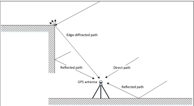
This phenomenon that distorts the signal with one or more replicas (depends on the environment) from nearby objects such as walls, buildings, vehicles, trees, water or ground surfaces, etc is called multipath. This means that, the receiver receives a sum of the original signal with other replicas with a different amplitude and phase. Because the multipath error depends on the antenna environment, this error is not consider as common source error and cannot be cancelled with the differential techniques. So this error is still a dominant error source in the precise GNSS based applications.
Figure 2.6 Multipath effect Adapted from Hannah (2001)
Multipath causes inaccurate measurement and even loss of lock on the signal. Two of the earliest methods in multipath elimination which are not always feasible, are the installation of antennas away from buildings, and using choke ring antennas, (Vaillon et al., 2000).
Apart from these two general methods which can be used in both static and dynamic modes, in this work we categorized solutions in two groups, stationary receiver and dynamic receiver. Some of previous works are as follows:
Stationary receiver:
• due to the repetition of geometry between GNSS satellites and receiver every sidereal day, the multipath pattern is also repeated in the same way. This fact can be used to mapping multipath error based on elevation and azimuth satellite angles. Another factor that helps to formulate and recognize this kind of error is that the replicated
signals always have a delay with respect to the Line Of Sight (LOS) signal. This is because of the longer path due to the reflection;
• another method is to use an adaptive filter to extract multipath error base on the GNSS repetition noise factor, (Ge, Han et Rizos, 2002).
Dynamic receiver:
• Excluding invisible satellites from the positioning computation is one way to mitigate the multipath error. Invisible satellite means a satellite that has been detected by the receiver but without LOS. This technique calculate the geometrical relation between satellites and the receiver by observing satellite positions using a satellite orbit simulator, (Marais, Berbineau et Heddebaut, 2005; Meguro et al., 2009). Additionally by calculating body frame heading angle with gyro or Inertial Measurement Unit (IMU) and observing obstruction position for example with an omnidirectional camera one can achieve a more accurate solution, (Meguro et al., 2009);
• Using a bandpass Finite Impulse Response (FIR) to extract multipath from the LOS signal is another method to mitigate the multipath error, (Han, Dai et Rizos, 1999);
• another method is based on signal to noise ratio value analysis, because not only the phase, but also the amplitude of the carrier phase signal is affected by multipath. So the SNR and the known antenna gain can be used for multipath mitigation, (Axelrad, Comp et Macdoran, 1996);
• another method is to use of Wavelet Transformation (WT), which is the transformation for non-stationary signals like GPS instead of Fourier Transform (FT). This method is close to the time-frequency analysis based on the Wigner-Ville distribution, (Chui, 2014; Satirapod et Rizos, 2005);
• various correlator techniques like narrow correlator can also reduce multipath errors, (Dierendonck, Fenton et Ford, 1992; Fenton et al., 1991).
2.4 Important parameters in satellite geometry
Apart from GPS measurements errors, satellite geometry and its associated parameters, is another important factor in the positioning solution accuracy. In this section, we discuss how to calculate satellite elevation and azimuth angle and quality metrics in the GPS constellation.
2.4.1 Elevation and azimuth
The azimuth and elevation angles are describe as the orientation of the line of sight vector with respect to the north, east and down of the user.
= [ ] (2.20)
where is the line of sight unit vector. Then:
= −arcsin( ) (2.21)
= arctan2( , ) (2.22)
Down East North Projection of line of sight in horizontal plane Line-of-sight vector Azimuth Elevation Ψ θ D u E u N u
Figure 2.7 Azimuth and elevation angles Adapted from Groves (2008)
2.4.2 Quality metrics of GNSS constellation
The position accuracy not only depends on the measurement accuracy and receiver quality but also depends on the satellite geometry. Figure 2.8 and Figure 2.9 clearly show the meaning of satellite geometry.
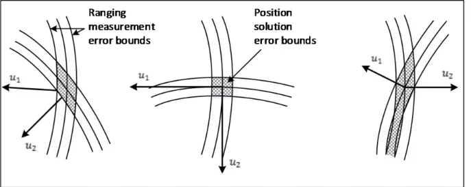
Figure 2.8 Effect of signal geometry on the position accuracy Adapted from Groves (2008)
In Figure 2.8, arcs show the average and the error bound for each ranging measurement, the shaded areas show the uncertainty bounds for the position solution and the vectors are the
line of sight vectors from user to satellites. The position solution is optimum when lines of sights are perpendicular. This effect is called Dilution Of Precision (DOP). Figure 2.9 shows the position of satellites in a poor and a good geometry.
Figure 2.9 Satellite geometry Adapted from Groves (2008)
In order to calculate DOP, a matrix of unit vectors line of sights for each satellite is created as follows: = −1 −1 −1 −1 (2.23) Q = (A A) = σ σ σ σ σ σ σ σ σ σ σ σ σσ σσ (2.24)
• Horizontal Dilution of Precision (HDOP):
= + (2.25)
• Position Dilution of Precision (PDOP):
= + + (2.26)
• Geometry Dilution of Precision (GDOP):
= + + + (2.27)
The GDOP lower than 1 is considered as a high level of confidence of data. Considering the calculated DOP values can help to interpret the achieved result.
2.5 Important references for GNSS navigation
Navigation in science terminology has two different meanings; the first one is to determination position or velocity of a moving object with respect to a known reference. The second one is to lead a moving user, a car, vessel or an airplane, from one location to another which is known as autopilot or guidance. In order to understand clearly the implementation part of this work, the more important navigation basics that have been used in this project is presented in this section.
Due to the importance of comparison between two frames in navigation, it is important to have a good understating of each frame. Some of important frames in navigation are as follows:
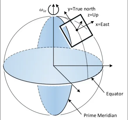
2.5.1 Earth centred earth fixed reference frame
The Earth Centred Earth Fixed (ECEF) reference frame is a commonly used navigation frame, on which their axis are fixed with respect to the earth and its origin is the mass center of the earth. The axis is pointing toward true North Pole (not the magnetic pole). The axis points toward the intersection of the equator and International Earth Rotation and Reference Systems Service (IERS) reference meridian which defines the zero degree longitude. The axis completes the right handed orthogonal set. This is an important reference frame in navigation because the axis is fixed with respect to the earth.
Figure 2.10 ECEF frame axis Adapted from Groves, 2008
2.5.2 Local frame
The local frame is a frame that is fixed with respect to a chosen position and its origin is the desired position (i.e. navigation system position or user position or the mass center of an object). The axis is always pointing toward the East and it is known as E axis. The axis is
the projection of the vector pointing to the North Pole into the orthogonal plane to the earth surface and it is known as North (N) axis. The z axis completes the right handed rule and it is known as Up (U) axis. This frame is an important frame in navigation because it is convenient to know the user's position with respect to the East, North, and Up.
Equator
Prime Meridian x=East y=True north
z=Up
Figure 2.11 Local frame, ENU Adapted from Groves (2008)
2.5.3 Body frame and Euler angles
This frame remains fixed with respect to the object body and its origin is at the mass origin of the object. The axis is in the direction of movement. The axis is the direction of gravity vector and the axis is the right handed orthogonal set. For the Euler angles, rotation about the axis is roll, the rotation about the axis is pitch and the rotation about the axis is yaw angle, Figure 2.12.
Figure 2.12 Body frame
2.6 Rotation Matrix
Rotation matrix is a 3 × 3 matrix which transforms a vector from a frame to another. In navigation this matrix defines a rotation from the body frame to the reference frame or vice versa which contains Euler angles as well.
A rotation matrix in general is called matrix and is defined as follow:
=
. . .
. . .
. . . (2.28)
=
cos cos cos
cos cos cos
where the upper index refers as "To" and the lower case refers to "From". is the unit vector of different axis [ , , ] and , is the angle between axis and .
For example the rotation matrix between ECEF and local navigation frame is as follows:
=
−sin cos −sin sin cos
−sin cos 0
−cos cos −cos sin −sin
(2.29)
In this thesis the rotation matrix will be frequently used in order to convert the baseline vectors from the ECEF frame to the local frame, from the local frame to the body frame and vice versa.
Now that an overview of the GPS, its measurements and associated errors, as well as the important references are presented, we go through different methods in the literature in order to choose the appropriate method. The next chapter presents an extensive literature review on the main challenging problems of this project namely ambiguity resolution and attitude determination.
CHAPTER 3 LITERATURE REVIEW
As we need a high precision solution for attitude determination, using carrier phase measurement which is more precise than the code measurements is necessary. The first important aspect to be able to use this measurement is to estimate the ambiguity parameter. The carrier phase measurement is ambiguous by an integer number of cycles from the satellite to receiver which remains constant until loss of lock. The section 3.1 presents the evolution of the GPS ambiguity resolution methods, as it is the first challenging problem in this scope. Then in the section 3.2, in order to find an appropriate method to estimate the attitude angles, a survey of attitude determination methods and comparison is presented. Finally, in the section 3.3, for increasing the solution accuracy and system reliability, a detailed study on how to incorporate the GLONASS measurements into the system is explained. For each module, first we go through the literature review of different methods and approaches then, summary for all the studied methods will be presented. At the end, a conclusion is provided for the findings of the entire chapter in the section 3.4.
3.1 Methods of GPS ambiguity resolution
Carrier phase measurement is the result of the phase difference of the received signal relative to the replica that is generated by the receiver. Therefore the fractional part of the phase difference can be measured within a millimetre accuracy (Verhagen et Teunissen, 2006), which is the reason why carrier phase measurement is much more accurate than code measurement. However the initial number of wavelengths from satellite to receiver is unknown and needs to be estimated for each satellite in view.
Since calculating the ambiguity of the carrier phase measurement is the key to use in high accuracy applications, we review here the most commonly used methods in literature.
Based on the literature, there are two main categories of ambiguity resolution methods consisting of (Crassidis, Lightsey et Markley, 1999; Teunissen, Giorgi et Buist, 2011):
• dynamic or motion-based;
• search-based, motionless or instantaneous.
The first category is dynamic or motion-based which uses a collected data set in a certain period in which the ambiguity remains constant and provides a batch solution. These methods are based on the satellite and body frame motion. These methods are not fast and they need high amount of memory to save the collected data and non-coplanar baselines, (Wang et al., 2009b). Despite these disadvantages, this method is highly reliable because of several criteria to accept the solution. Statistical checks of the error and considering the closeness of the floating point solution and the actual integers are among those criteria (Crassidis, Lightsey et Markley, 1999).
The second category which is usually called motionless or instantaneous or search-based methods are based on estimating a set of integers of one epoch and search for the best solution, (Hatch, 1991; Park et Teunissen, 2003). Due to the high convergence speed, this method is a suitable method for real time applications, (Li et al., 2004; Park et Teunissen, 2003), but since it can converge to an incorrect solution in the presence of noise especially multipath, all solutions should be checked several times before selecting the final solution, (Teunissen, 1997; Yoon et Lundberg, 2002). The instantaneous category, consists of three steps: float solution, integer ambiguity resolution and integer ambiguity validation. The first step usually is the result of an estimation process consisting of estimation the ambiguity in real numbers. The second step can be done with three types of methods: Simply rounding,
integer bootstrapping and Integer Least-Squares (ILS) estimator, (Zheng, 2010). The
instantaneous category can be divided into three types of search domains, (Kim et Langley, 1999):
1. The measurement domain: It uses the C/A code or P-code directly to calculate the integer ambiguity of the corresponding carrier phase measurement. In order to
achieve this ambiguity with a proper accuracy, usually observation combination of L1 and L2 is needed, (Cocard et Geiger, 1992; Collins, 1999);
2. The coordinate domain: The coordinate domain is the biggest subcategory in the instantaneous category. Many ambiguity search methods are in this category such as: Least-Squares Ambiguity Search Technique (LSAST), Fast Ambiguity Search Filter (FASF), Ambiguity Function Method (AFM), Fast Ambiguity Resolution Approach (FARA), (Kim et Langley, 2000);
3. The ambiguity domain: The ambiguity domain is known as an efficient with high success rate method and has recently received lots of attention. This method is based on the original search domain transformation in ambiguity domain which is easier and faster to solve, (Teunissen, Giorgi et Buist, 2011). LAMBDA is the most important and well known method in the ambiguity domain.
The different methods of ambiguity resolution are not comparable and even is not always feasible, (Kim et Langley, 2000). We describe all these methods briefly as follows:
3.1.1 Ambiguity function method
(Counselman et Gourevitch, 1981) has proposed this technique and (Remondi, 1991) has improved it. Since the Ambiguity Function Method (AFM) uses the fractional value of the carrier phase, and triad positions are searched instead of triad ambiguity set, it is insensitive to cycle slip which makes it different from other methods, (Hofmann-Wellenhof, Lichtenegger et Collins, 2013; Kim et Langley, 2000; Park et al., 1996).
This technique is based on geometric change between satellite and receiver, (Hofmann-Wellenhof, Lichtenegger et Collins, 2013). In case of cycle slip, despite other methods, AFM can continue the calculation without any interruption or reinitialisation. As a result, this feature significantly improves the computational time of this method.
It is proved that the effectiveness and accuracy of the solution barely changes with loss of lock and even when data is absent for a long time, which means a few minutes of data at any time plus a few minutes one hour later is almost the same with one hour data without interruption, (Lu, 1995). However, this method takes high computational time, 1 to 2 minutes and consequently it is not a suitable method for real time applications, (Lu, 1995).
3.1.2 Least-squares ambiguity search technique
The early studies in this method is done by (Beutler et al., 1984) and (Wei, 1986). In this method, each double difference ambiguity term from each satellite is considered as an independent parameter. All these unknown parameters, take time for finding a search space and the fixed number.
One of the main disadvantages of this method is its heavy computational burden, which makes it unusable method for On-The-Fly (OTF) ambiguity resolution. (Hatch, 1989) and (Hatch, 1991) proposed a method to overcome this inconvenience by limiting the number of independent parameters to three and adding one check before acceptance of the solution. For satellite, there are − 1 double difference ambiguity parameters, so for example, for having three independent ambiguities, four satellites have to be chosen based on the PDOP value. The search space cube is calculated by theses four satellites which are known as primary satellites. The rest of satellites which are called secondary satellites are usually used as to check on each potential ambiguity set in the search space. Chi-square test usually is applied for each ambiguity set. If more than one ambiguity set is passed, due to the noise or bad geometry of satellites, this test can help to approve the solution for the next epoch. Gaussian error distribution is assumed in this method. Due to 3 dimensional ambiguity search space regardless of the number of tracked satellites, this method is fast in computational time, thus it is suitable for real time application, (Lu, 1995).
3.1.3 Fast ambiguity resolution approach
This technique is proposed by (Frei et Beutler, 1989) and it consists of four steps to obtain the solution:
1. First Step is to estimate the ambiguity based on the carrier phase measurement and
by an adjustment procedure with corresponding covariance matrix of the unknown parameters and the standard deviation of the ambiguity numbers,
(Landau et Euler, 1992);
2. Second Step is to determine the search space based on standard deviation and
ambiguity correlation. This means by having as standard deviation of ambiguity , ± is the search range for this ambiguity where is statistically calculated from Student’s t-distribution;
3. Third step is to perform a least-squares adjustment for each ambiguity set that is
accepted statistically;
4. Final step is to pick the solution with smallest variance and compare it with the float
solution. If the solution is compatible, this set will be accepted.
3.1.4 Fast ambiguity search filter
(Chen, 1993) proposed this method and further investigations were made by (Chen et Lachapelle, 1995). This method uses Kalman filter as an estimator with the ambiguity parameters in the state vector. As soon as the ambiguity parameters are set with a proper level of confidence, they are treated as fix known integers. After that, in order to determine the search space, for example for the second ambiguity parameter, the first ambiguity is considered as known integer and removed from the state vector. For determining the third ambiguity search space, the first and the second ambiguities are considered known and fix integers. This procedure will be performed for all the ambiguities, one by one, and because of that, it is called a recursive method.
After fixing all the ambiguities, they are treated as known parameters and they will be removed from the state vector. Other unknown parameters, which are the coordinates of the receivers, will be replaced then into the state vector, unknown parameter. So the receiver's coordinates can be calculated more precisely.
This technique uses full information of satellite geometry and the ambiguity search space for each satellite is calculated not only recursively but also based on other integer ambiguities. Consequently, two important factors to OTF ambiguity resolution which are computational and observational time, are significantly reduced compare to the least-squares method, (Chen et Lachapelle, 1995).
3.1.5 Least-squares ambiguity decorrelation adjustment
One of the most powerful ambiguity resolution method is LAMBDA, which was proposed by (Teunissen, 1995). This method is different from FASF, FARA, and AFM in search space transformation and it is known as an efficient method with maximum success rate, (Teunissen, 1995; Zheng, 2010).
In this method, each baseline can be written in a linearized model as, (Wang et al., 2009a):
= + + (3.1)
where is the measured minus computed double difference GPS carrier phase measurement, is the double difference ambiguity vector, is the baseline component, is the noise vector, and and are the design matrices.
First and with their covariance matrices should be estimated with least-squares method as:
a b
Q Q
Q Q (3.2)
Then the optimal solution of the Equation (3.1) will be:
min‖ − ‖ , ∈ ℤ (3.3)
Due to the cross-correlation of the ambiguities in the original search space, the search space is extremely elongated and it takes a long time to determine the ambiguity with high level of accuracy. This dependency can be seen as a discontinuity in the spectrum of ambiguity conditional variances, and it will be far more problematic in the short observation time span and in the absence of the P-code, (Teunissen, 1995).
LAMBDA overcomes this problem by performing a Z-transformation in order to decorrelate the cross-correlation between ambiguities while preserving the integer nature of the problem. This method reformulates the original search space by decorrelating via a Z-transformation into another search space, which is easier to solve and it is faster. LAMBDA converts the elongated space to a round (spherical) space, the search space then will be aligned to the grid axes and can be simply estimated by rounding to the nearest integer, (Teunissen, 1995). The transformed search space of Equation (3.3) can be written as:
( ̂ − ) ̂ ( ̂ − ) ≤ (3.4)
where ̂ = and the ̂ = and the is the size of the search ellipsoid. The size
of is determined by = [ ]. The boundary of the search space is an ellipsoid centered at ̂, its shape is defined by covariance matrix ̂ and its size is determined by , (Zheng, 2010).
The idea of the search strategy is the same with other search-based methods but it is different in integer ambiguity resolution (second step). After the transformation, a sequential conditional least-squares is then performed.
Size of the search space is a critical issue because the small one may not contains the correct integer ambiguity and the large one takes a long time to converge. However, this method has been developed for unconstrained or linearly constrained, which is not necessarily optimal for GNSS attitude determination specially for those with rigid platform, (Teunissen, Giorgi et Buist, 2011).
Some notes about ambiguity resolution methods:
• according to (Kim et Langley, 2000), there is another way to categorize the ambiguity resolution method. We can split up the problem into all ambiguity search method like FARA, FASF, LAMBDA, modified Cheloskey decomposition method and independent ambiguity search method like LSAST. In the first category, all the ambiguity parameters will be searched but in the second category, first independent ambiguities should be fixed and dependent ambiguities will be fixed after based on independent parameters;
• a long time span is usually needed to converge the ambiguity solution especially in single frequency and low-cost system because the observations are taken at low rate and errors are highly correlated, (Zheng, 2010);
• there are three fundamental properties that should be targeted, in order to select a suitable method, (Campo-Cossio et al., 2009):
- initial attitude independent;
- high success rate estimation;