HAL Id: hal-01025664
https://hal.archives-ouvertes.fr/hal-01025664
Submitted on 18 Jul 2014HAL is a multi-disciplinary open access archive for the deposit and dissemination of sci-entific research documents, whether they are pub-lished or not. The documents may come from teaching and research institutions in France or abroad, or from public or private research centers.
L’archive ouverte pluridisciplinaire HAL, est destinée au dépôt et à la diffusion de documents scientifiques de niveau recherche, publiés ou non, émanant des établissements d’enseignement et de recherche français ou étrangers, des laboratoires publics ou privés.
In vitro Analysis of Localized Aneurysm Rupture
Aaron Romo, Pierre Badel, Ambroise Duprey, Jean-Pierre Favre, Stéphane
Avril
To cite this version:
Aaron Romo, Pierre Badel, Ambroise Duprey, Jean-Pierre Favre, Stéphane Avril. In vitro Analysis of Localized Aneurysm Rupture. Journal of Biomechanics, Elsevier, 2014, 47 (3), pp.607-616. �hal-01025664�
In vitro Analysis of Localized Aneurysm Rupture
1
2 3 4
Aaron Romo1, Pierre Badel1, Ambroise Duprey2, Jean-Pierre Favre2, Stéphane Avril1
5
1
Ecole Nationale Supérieure des Mines de Saint-Etienne, CIS-EMSE, CNRS:UMR5146, LCG, F-42023 Saint Etienne, France
6
2
Hôpital Nord, Cardiovascular Surgery Service, CHU de Saint Etienne, F-42055 Saint-Etienne cedex 2, France.
7 8 9 10 Corresponding author: 11 Aaron Romo 12
Center for Health Engineering
13
Ecole Nationale Supérieure des Mines
14
158 cours Fauriel
15
42023 SAINT-ETIENNE CEDEX 2 France
16 Phone: +33477429329 17 Fax: +33477499755 18 Email: romo@emse.fr 19 20 21 22 KEYWORDS 23 24
Aneurysm, human aorta, inflation test, rupture, ultimate stress.
25 26 27 28
word count (introduction through acknowledgments): 3511
29 30
ABSTRACT
3132
In this study, bulge inflation tests were used to characterize the failure response of 15 layers of
33
human ascending thoracic aortic aneurysms (ATAA). Full field displacement data were collected
34
during each of the mechanical tests using a digital image stereo-correlation (DIS-C) system. Using the
35
collected displacement data, the local stress fields at burst were derived and the thickness evolution
36
was estimated during the inflation tests. It was shown that rupture of the ATAA does not
37
systematically occur at the location of maximum stress, but in a weakened zone of the tissue where
38
the measured fields show strain localization and localized thinning of the wall. Our results are the
39
first to show the existence of weakened zones in the aneurysmal tissue when rupture is imminent.
40
An understanding these local rupture mechanics is necessary to improve clinical assessments of
41
aneurysm rupture risk. Further studies must be performed to determine if these weakened zones can
42
be detected in vivo using non-invasive techniques.
43 44 45 46 47 48 49
INTRODUCTION
5051
Each year thoracic aneurysms are diagnosed in approximately 15,000 people in the United States and
52
more than 30,000 people in Europe (Clouse 1998). Of this number 50-60% are ascending thoracic
53
aortic aneurysms (ATAA) (Isselbacher 2005). However the rupture of the ATAA remains an almost
54
unexplored topic. ATAAs are caused by the remodeling of the arterial wall and they rupture when the
55
stress applied to the aortic wall locally exceeds its capacity to sustain stress (Vorp et al., 2003).
56 57
In an attempt to understand the mechanical behavior of the aortic tissue; different authors have
58
performed mechanical tests. Uniaxial tensile tests were performed by (Mohan and Melvin, 1982) on
59
healthy descending aortic specimens; they concluded that the most reasonable failure theory for
60
aortic tissue was the maximum tensile strain theory. (He and Roach, 1994) also performed uniaxial
61
tensile tests and showed that aneurysms were less distensible and stiffer than healthy tissues. Using
62
uniaxial tensile tests to compare healthy tissues with ATAA specimens (Garcia-Herrera et al., 2011)
63
concluded that the age, beyond the age of 35, was the cause of significant decrease of rupture load
64
and elongation at failure. They found no significant differences between the mechanical strength of
65
aneurysms and healthy tissues. In contrast, (Vorp et al., 2003) found a significant decrease in the
66
tensile strength of the ATAA specimens and concluded that its formation was associated with the
67
stiffening and weakening of the aortic wall. Providing data on the mechanical behavior in the
68
physiological range, (Duprey et al., 2010) found that the aortic wall was significantly anisotropic with
69
the circumferentially oriented samples being stiffer than the axial ones.
70
71
The biaxial mechanical behavior of the aortic tissue has been investigated with bulge inflation tests.
72
Dynamic and quasi-static bulge inflation tests (Mohan and Melvin, 1983) were performed on healthy
73
descending aortas. The failure of the aortic tissue always took place with a tear in the circumferential
74
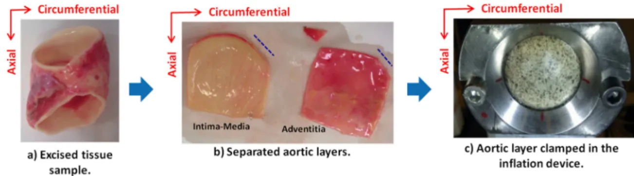
direction. Similarly, (Marra et al., 2006) performed inflation tests using porcine healthy aortic tissues,
showing that the rupture occurs with a crack oriented in the circumferential direction of the artery.
76
More recently (Kim et al., 2012) performed inflation tests using ATAA specimens. Material
77
parameters were identified using the virtual fields method (Grédiac et al., 2006; Avril et al., 2010)
78
and the average Cauchy stress values at which the rupture occurred were derived for all the
79
specimens.
80 81
None of the studies mentioned above analyzed locally the rupture of the tissue from its first
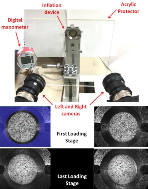
82
initiation. Moreover, all these studies derived an average stress estimation across the specimens and
83
none were able to show if the rupture initiates at the location of maximum stress or if the rupture
84
was triggered by the existence of weakened parts within the tissue. Our objective was to address
85
this issue by carrying out full-field measurements in human ATAA specimens tested in a bulge
86
inflation test up to failure. In order to determine the cause and location of the rupture, thickness
87
evolution estimations and local stress distributions were calculated during the inflation of the
88
specimens.
89 90 91
METHODS
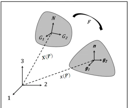
9293
Sample Preparation and Experimental Protocol
94
ATAA specimens were obtained from donor patients who underwent surgical replacement of their
95
ATAA with a synthetic graft. The collection of the aortic tissues was done in accordance with the
96
guidelines of the Institutional Review Board of the University Hospital Center of Saint-Etienne.
97
Specimens were kept at 4 °C in 0.9% physiological saline solution and testing was completed within
98
24 hours of tissue harvest (Adham et al. 1996). Table 1 lists the demographic information for the
99
collected ATAA specimens.
100
101
Each ATAA (Fig. 1-a) was cut into square specimen approximately 45 x 45 mm. Each specimen was
102
then separated into two layers: intima-media and adventitia (Fig. 1-b). The average thickness of each
103
layer was measured using digital calipers; the layer of interest was put between two plastic plates
104
and the thickness of the layer and the plates was measured. Then the thickness of the two plates was
105
subtracted from the measured value. The ATAA layer was clamped in the inflation device so that the
106
luminal side of the tissue faced outward and the circumferential direction of the artery coincided
107
with the horizontal axis of the clamp (Fig. 1-c). Finally a speckle pattern was applied to each sample
108
using black spray paint (Fig. 1-c). Note that the luminal side of each layer was chosen to face outward
109
since the adventitial surface was highly irregular making difficult for the speckle pattern to adhere to
110
the surface.
111 112
A hermetically sealed cavity was formed between the clamped ATAA layer and the inflation device.
113
During the inflation test, water was injected at a constant rate by pushing a piston pump at 15
114
mm/min until the tissue ruptured. Simultaneously, the pressure was measured with a digital
115
manometer (WIKA®, pressure gauge DG-10). Images were recorded using a commercial DIS-C system
116
(GOM®, ARAMIS 5M LT) at every 3 kPa, until the sample ruptured (Fig. 2). The DIS-C system was
composed of two 8-bit CCD cameras equipped with 50 mm lenses (resolution: 1624 x 1236 px). In
118
this study, 15 ATAA layers were successfully tested until rupture. Only the specimens that ruptured in
119
their central area (without touching the boundaries of the inflation device) were used.
120 121
Data Analysis
122
Once the experimental procedure was completed, image processing was performed using Aramis®
123
software. In each of the acquired images (Fig. 2), the area of interest (AOI), which was a circle
124
measuring 30 mm diameter, was identified. A facet size of 21 px and a facet step of 5 px were chosen
125
based on the speckle pattern dot size, distribution, and contrast. The selected facet size and step
126
yielded a resolution of 0.54 µm for in-plane displacements and 1.5 µm for the out-of-plane
127
displacement.
128
129
To capture the kinematics of the membrane (Naghdi 1972; Green and Adkins 1970; Lu et al., 2008)
130
we define the position vectors for a material point in the initial and deformed configurations as
131
( ) and ( ), respectively (Fig. 4). The surface is parameterized using a pair of surface coordinates
132
( ) = ( ) ∙ where are the basis vectors of the global coordinate system GCS (Fig. 3) and
133
= 1,2. The local covariant basis vectors and for the deformed and initial configurations,
134
respectively, are found using the following relationships:
135 136
= ξ = ξ (1)
137
The local contravariant basis vectors and are then defined as:
138 139
= ξ = ξ (2)
The two-dimensional deformation gradient, , is calculated from the current and initial basis vectors:
141 142
= ⊗ (3)
143
Then, at each material point, the two- dimensional Green-Lagrange strain, , is determined:
144 145
=12 ( − ) (4)
146
To define the three-dimensional deformation, we set = ℎ ℎ⁄ , where ℎ and ℎ are the thicknesses
147
in the deformed and undeformed configurations, respectively, and required the transverse shear
148
strains to vanish. It follows that the three dimensional deformation gradient and Green-Lagrange
149
strain tensor are given by:
150 151
= ⊗ + " ⊗ # =$%& ' ⊗ '+ % # ⊗ # − ( (5)
152
where " and # are outward unit normals to the surface in the current and initial configurations,
153
respectively.
154 155
Determination of the Local Stress Fields
156
The aneurysm wall is modeled as a nonlinear elastic membrane. A unique feature of modeling the
157
aneurysm wall as a nonlinear elastic membrane is that the tension in the vessel wall can be
158
determined without the use of a constitutive model to describe the elastic properties of the wall (Lu
159
et al., 2008). The local equilibrium equations for the elastostatic problem may be written as (Lu et
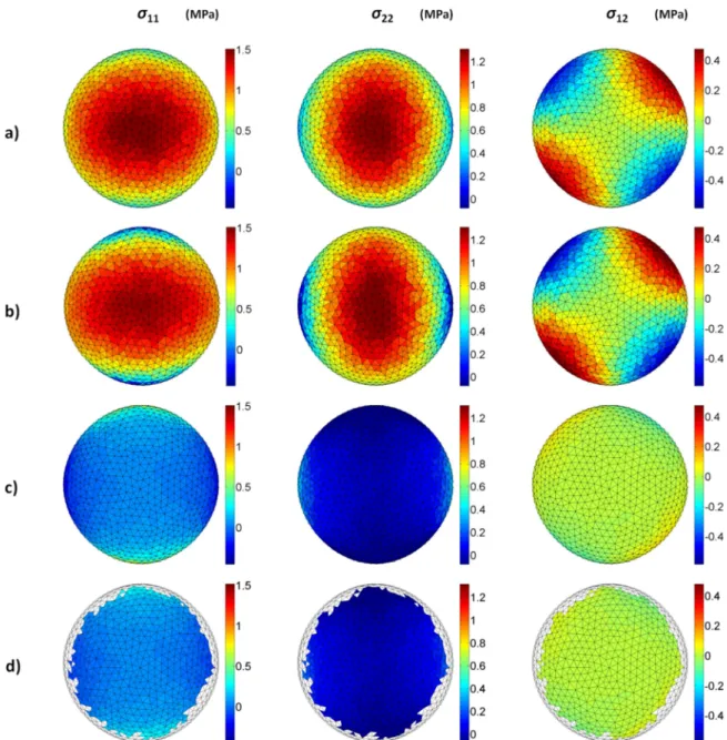
160
al., 2008; Zhao 2009):
161 162
1
) &) ℎ* ' (,'+ +" = , (6)
163
where = det ( . ') is the determinant of the metric tensor, ℎ is the current thickness, + is the
164
internal pressure applied for the inflation and * ' are the unknown components of the Cauchy
165
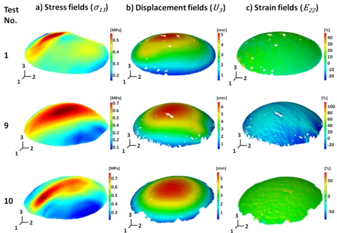
stress tensor 1 in the local covariant basis. Note that Eq. (6) is in tensorial form and the Einstein
166
summation convention is used. Then, we approximate the spatial variations of all the quantities of
167
Eq. (6) using linear shape functions of the surface coordinates which take on a null value at all nodes
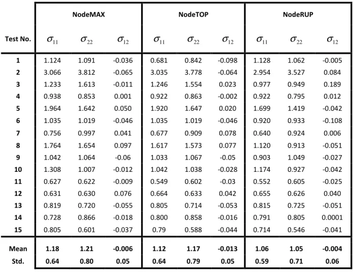
168
of the mesh except at node 2 where it is 1. The shape functions are defined on a triangular finite
169
element mesh having 3 elements and 4 nodes (Fig. 5).
170 171
Using this approximation scheme, Eq. (6) is written at the centroid of each element, which yields:
172 173 1 1 3 ∑78$) ( 7) 9 :) ( 7)ℎ(;7)* '( 7) ( 7)<=< '7> 78$ + +13 9 "( ?) 78$ = , (7) 174 where @AB
@CD are the shape function derivatives at the centroid of the element and where the Einstein
175
summation convention still applies for indexes and E. Eq. (7) is then projected into the GCS and the
176
procedure is repeated for each triangular element. A linear system of 33 equations is produced. It
177
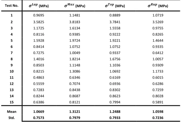
contains 34 unknowns which are the 3 components of the Cauchy stress tensor in the local covariant
178
basis at the 4 nodes of the mesh. A convergence study showed that a mesh with 3=1203 elements
179
and 4=644 nodes was a good compromise between precision and time of calculation.
180 181
The system was completed by a set of equations on the boundaries of the tested area, where it was
182
assumed:
183 184
(1 ∙ F) ∙ " = 0 (8)
(1 ∙ F) ∙ H = 0 (9)
185
where H, F, " defines a local basis at the boundaries (Fig. 5-b) with I is tangent to the boundary, " is
186
an outward unit normal vector to the surface and F = "⊗ H is chosen to make the local coordinate
187
system right-handed. Along the boundaries, Eq. (8) sets the traction vector perpendicular to ,
188
allowing in-plane tractions only and Eq. (9) sets the traction vector perpendicular to I , allowing no
189
shear on the boundary. The resultant boundary traction automatically balances the total pressure
190
applied on the wall due to the local equilibrium equation (Eq. (6)) written for each element. The final
191
over-determined linear system of equations was solved in the least-squares sense.
192 193
The calculated components of the stress tensor are finally projected in the orthonormal local
194
coordinate system (LCS) ( JK, JL, JM ) defined such that:
195 196 J = " J%=‖ % %‖ (10) J$= J% ⊗ J 197
where " is again the outward unit normal to the surface.
198 199
The stress was analyzed at three locations:
200 201
• NodeMAX: node with the largest stress eigenvalue
202
• NodeTOP: node at the top of the inflated membrane
203
• NodeRUP: node where rupture initiates
205
At NodeMAX and NodeTOP locations, the largest eigenvalue of the Cauchy stress tensor (largest
206
principal stress) were found and denoted *OPQ and * RS, respectively. At NodeRUP, the stress in the
207
direction perpendicular to the crack that occurs at rupture was computed:
208 209
*TUS= (1 ∙ VW) ∙ VW (11)
210
where VW is the unit vector perpendicular to the rupture (Fig. 8c). It is derived for each specimen
211
using the images obtained from the DIS-C system at the moment of the rupture. Using a custom
212
MatLab® code, a series of points were manually placed on an image of the ruptured edge. A linear
213
regression was then performed using those points and the angle between the fit line and the
214
horizontal axis was calculated.
215 216
Finite Element Validation Study
217
Using a mesh size of 3=1203 elements and 4=644 nodes, a validation analysis was performed (see
218
Appendix A for details). The stress distributions obtained from a finite element analysis (FEA) were
219
defined as reference values and compared with the stress distributions obtained using the present
220 approach. 221 222 Thickness Evolution 223
At every pressure step, the current thickness of each element was calculated. The aneurysmal tissue
224
was modeled as incompressible membrane therefore the following relationship holds between the
225
initial thickness, ℎ , and the current thickness, ℎ.
226 227
ℎ =X ℎ
$$X%%− X%$X$% (12)
228
We note that the ex vivo thickness, ℎ , was assumed to be initially homogeneous and that X$$, X%%,
229
X%$ and X$% are the components of the deformation gradient tensor (Eq. (3)).
230 231
Laplace’s Law
232
Laplace’s Law (Peterson et al., 1960; Humphrey 2002) was used to calculate a global estimate of the
233
ultimate stress for each ATAA layer by assuming the sample was a hemisphere
234 235
*YPS= +Z
2ℎ (13)
236
where + was the inflation pressure, Z was the radius of curvature estimated using a least-squares
237
surface fitting of the inflated shape, and ℎ was the average current thickness of the elements in the
238 mesh. 239 240 241
RESULTS
242 243The stress distributions obtained from the FEA simulation (Fig. 6-a) were compared with the stress
244
distributions obtained using the present approach (Fig. 6-b). The mean absolute error (Fig. 6-c) was
245
calculated revealing that the largest errors occurred at the boundaries. Ignoring the elements at the
246
boundaries, the average error was significantly reduced to 0.8%, 1.4%, and 0.8% for *$$, *%%, and
247
*$%, respectively (Fig. 6-d). This showed that the stress estimates contain some errors along the
248
border due to the assumed boundary conditions but these errors vanish rapidly away from the
249
border. For this reason, only the tests where the rupture occurred at a distance of more than three
elements away from the border were included in this study.
251 252
Using the approach we have presented, the components of the Cauchy stress tensor were calculated
253
at every node for each 3 kPa pressure step until the sample ruptured (Fig. 7-a). The displacement
254
(Fig. 7-b) and strain fields (Fig. 7-c) used to calculate the stress and thickness evolution are also
255
shown.
256 257
In Table 2 we report the three components of the Cauchy stress tensor. Our results (mean ± std) for
258
*$$ were 1.18 ±0.64 MPa at NodeMAX, 1.12 ±0.64 MPa at NodeTOP and 1.06 ±0.59 MPa at
259
NodeRUP. The values for *%% were 1.21 ±0.80 MPa at NodeMAX, 1.17 ±0.79 MPa at NodeTOP and
260
1.05 ±0.71 MPa at NodeRUP.
261 262
In Fig. 8-a, we show the thickness distribution (Eq. (12)) one pressure step before rupture for five
263
tests. For each of the samples thick (dark red) and thin (dark blue) regions can be identified. The
264
locations of NodeMAX, NodeTOP, and NodeRUP for these five tests are also shown in Fig. 8-b.
265
Contrary to the generally accepted theory that the rupture occurs at the location of the maximum
266
stress, the experimental results show that rupture often initiates at a different location (NodeRUP),
267
possibly due to the non-homogeneous strength of the tissue. An image of the ruptured layer is
268
shown in Fig. 8-c, where the magenta points and the blue regression line were used to determine the
269
rupture angle, [.
270 271
Table 3 and Fig. 9 summarize the three ultimate stress values (*OPQ, * RS, and *TUS) calculated at
272
their corresponding locations (NodeMAX, NodeTOP and NodeRUP) compared with *YPS (Eq. (13)).
273
For the six adventitia layers, the average stress values (mean ± std) were 1.49 ±1.06 MPa, 1.76 ±1.07
274
MPa, 1.69 ±1.10 MPa, and 1.46 ±1.03 MPa for *YPS, *OPQ, * RS, and *TUS, respectively. For the
275
remaining nine media layers, the average stress values were found to be 0.78 ±0.26 MPa, 1.01 ±0.36
MPa, 0.95 ±0.31 MPa, and 0.78 ±0.20 MPa for *YPS, *OPQ, * RS, and *TUS, respectively. The four
277
calculated ultimate stress values were higher for the adventitia layers, confirming its role of
278
structural support of the artery (Fung, 1993).
279 280 281
DISCUSSION
282 283Comparison with Existing Literature 284
Other investigators performing inflation tests have reported rupture stresses between 0.751 and
285
1.75 MPa (Kim et al., 2012, Mohan and Melvin, 1983, Marra et al., 2006). In the present study the
286
rupture stress, *TUS, was on average 1.46 MPa for the adventitia layers and 0.72 MPa for the media
287
layers. The results obtained from our analysis were reasonable and lie within the range of reported
288
values in the literature. It must be noted that our results were twice as large of those of Kim et al.
289
(2012) who found 0.751 MPa for adventitia layers and 0.39 MPa for media layers. This can be
290
explained by the different methods used to calculate the rupture stress. While Kim et al. (2012)
291
assumed a constant thickness throughout the inflation, the present method was capable of
292
estimating the thickness evolution of the sample (Eq. (12)). Based on the large changes in thickness
293
observed in the samples (Fig. 10), it was expected that our values would be significantly larger than
294
those reported by Kim et al. (2012).
295 296
Comparison of the Ultimate Stress at Different Locations 297
The stress found using Laplace’s Law, *YPS, in Eq. (13) was considered a global estimate of the
298
rupture stress, since it was computed using a global radius of curvature and the mean thickness of
299
the inflated ATAA layer. A comparison between this global stress value and the calculated local stress
300
values, *OPQ, * RS, and *TUS, was done as the majority of published studies have not calculated
301
local stress distributions. The stress calculated from Laplace’s Law was frequently smaller than the
other local stress values. The difference can likely be explained by differences in the thickness
303
calculation. On the one hand Laplace’s Law uses the average current thickness of the entire inflated
304
aortic layer while the three local stress values use the current local thickness of the element where
305
the node concerned was located.
306 307
Detection of Weakened Zones in the Tissue 308
In every test rupture was preceded by significant local deformation and reduction of the thickness.
309
This phenomenon was clearly illustrated in Fig. 8, where local thinning was observed at the rupture
310
location. Occasionally the maximum stress value was located in the weakened area, but more
311
frequently it was located elsewhere. This led us to hypothesize that the ATAA layers had weakened
312
regions that caused the localized thinning of the layer during the inflation test. When observing the
313
evolution of the ATAA layer thickness (Fig. 10), the region where the rupture was most likely to occur
314
could be observed many stages before the rupture. Moreover, the orientation of the rupture always
315
appeared in the same direction as the thickness heterogeneity in the inflated ATAA layer.
316 317
Main Sources of Variability 318
It was noticed that test number 2, an adventitia layer, had by far the highest ultimate stress values.
319
Possibly explained because this layer was the thinnest of all the tissue samples and the donor patient
320
was 36 years old, which made him by far the youngest patient donor (mean age: 66 years).
321 322
Limitations 323
a) Comparison with healthy tissue 324
Due to the difficulty of obtaining healthy ascending aortic specimens, there was no comparison
325
between healthy aorta and ATAA specimens. As many authors have noticed (Choudhury et al., 2008;
326
Cinthio et al., 2006; Prehn et al., 2009), this comparison can help understanding the causes of the
327
pathology.
329
b) Initial thickness measurement 330
The measurement of the ex vivo initial thickness ℎ of the ATAA tissue was an average estimate of
331
the thickness of the tissue. Measuring the thickness of the specimen at various locations in the tissue
332
was precluded as the sharp shape of the caliper can easily penetrate the soft tissue and damage the
333
tissue. The tests method could be further improved in the future by incorporating a technique
334
capable of capturing the location dependent thickness of the tissue. Other techniques such as, for
335
example, a PC-based video extensometer (Sommer et al., 2008) or a non-contact laser beam
336
micrometer (Iliopoulos et al., 2009) could be used to measure the thickness of the aortic tissue at
337
multiple locations.
338 339
c) Effect of the loading conditions 340
A finite element study was undertaken to show that the traction boundary conditions used in our
341
simulation (Eqs. 9-10) only minimally affected the stress calculations in the center region of the
342
specimen. Due to boundary effects, the present approach is limited to characterizing rupture
343
phenomenon occurring far from the boundaries. In the future it would be useful to improve the
344
precision by implementing an approach similar to Zhao (2009) who defined a boundary-effect-free
345
region where the calculated stress distribution remains invariant.
346 347
d) Pure membrane assumption 348
Using the present approach, the average stress across the thickness of the inflated ATAA layer was
349
calculated. The assumption of a pure membrane behavior is justified when the concerned tissue is
350
subjected to tensile extension, and is physically thin enough so the transverse shear and the
across-351
thickness stress variation are safely ignored (Horgan and Saccomandi 2003, Lu et al. 2008). Based on
352
the validation analysis (Appendix A), the stress distribution calculated using the present approach
353
was in very good agreement with the average stress distribution calculated between the outer and
inner surface using Abaqus® software. This indicates that the pure membrane assumption does not
355
affect the reconstruction of this average stress across the thickness.
356 357 358
CONCLUSIONS
359 360In this manuscript, we have used a straight forward approach to investigate the in vitro rupture
361
behavior of ATAA layer during an inflation test. The main advantage of our approach was that local
362
stress field for the ATAA layer was obtained without requiring any material properties. Our results
363
showed that rupture in the ATAA inflated layers was more prone to occur in regions where the layer
364
was weakened. The majority of the time, rupture occurs where the thickness of the layer has been
365
reduced the most. Using maps of the local thickness as a function of pressure one can easily predict
366
the rupture location. Future studies must be conducted to determine if the localized thinning
367
observed in these experiments can also be observed in vivo using techniques such as magnetic
368 resonance imaging. 369 370 371
ACKNOWLEDGEMENTS
372 373The authors would like to acknowledge the National Council on Science and Technology of Mexico
374
(CONACYT) for funding Mr. Romo’s scholarship. We also would like to thank Dr. Frances Davis for her
375
helpful suggestions to improve the quality of the paper.
376 377 378
CONFLICT OF INTEREST
379380 None 381 382 383
REFERENCES
384 385Adham, M., Gournier, J., Favre, J., De La Roche, E., Ducerf, C., Baulieux, J., Barral, X., Pouyet, M.,
386
1996. Mechanical characteristics of fresh and frozen human descending thoracic aorta.
387
Journal of Surgical Reaserch, 64(1), 32-34.
388
Avril, S., Badel, P., Duprey, A., 2010. Anisotropic and hyperelastic identification of in vitro human
389
arteries from full-field measurements. Journal of Biomechanics 43(15), 2978-2985.
390
Choudhury, N., Bouchot, O., Rouleau, L., Tremblay, D., Cartier, R., Butany, J., Mongrain, R., Leask, R.,
391
2008. Local mechanical and structural properties of healthy and diseased human ascending
392
aorta tissue, Cardiovascluar Pathology 18, 83-91.
393
Cinthio, M., Ahlgren, A., Bergkvist, J., Jansson, T., Persson, H., Lindstrom, K., 2006. Longitudinal
394
mouvements and resulting shear strain of the arterial wall. American Journal of Physiology -
395
Heart and Circulatory Physiology 291, H394-H402.
396
Clouse, W., Hallett, J., Schaff, H., Gayari, M., Ilstrup, D., Melton, L., 1998. Improved prognosis of
397
thoracic aortic aneurysms: a population-based study. Journal of the American Medical
398
Association 280, 1926-1929.
399
Duprey, A., Khanafer, K., Schlicht, M., Avril, S., Williams, D., Berguer, R., 2010. In vitro
400
characterization of physiological and maximum elastic modulus of ascending thoracic aortic
401
aneurysms using uniaxial tensile testing. European Journal of Vascular and Endovascular
402
Surgery 39, 700-707.
403
Fung Y., 1993. Biomechanics: mechanical properties of living tissues. Springer, New York.
404
Garcia-Herrera, C., Atienza, J., Rojo, F., Claes, E., Guinea, G., Celentano, D., Garcia-Montero, C.,
405
Burgos, R., 2012. Mechanical behaviour and rupture of normal and pathological human
406
ascending aortic wall. Medical & Biological Engineering & Computing 50, 559-566.
407
Grédiac, M., Pierron, F., Avril, S., Toussaint, E., 2006. The virtual fields method for extracting
408
constitutive parameters from full-field measurements: a review. Strain 42(4), 233-253.
409
Green, A., and Adkins, J., 1970. Large elastic deformations. Clarendon Press, Oxford.
410
He, C.M., Roach, M.R., 1994. The composition and mechanical properties of abdominal aortic
411
aneurysms. Journal of Vascular Surgery 20, 6-13.
412
Holzapfel, G., Gasser, T., Ogden, R., 2000. A New Constitutive Framework for Arterial Wall Mechanics
413
and a Comparative Study of Material Models. Journal of Elasticity, 61(1), 1-48.
414
Horgan, C., and Saccomandi, G., 2003. A description of arterial wall mechanics using limiting chain
415
extensibility constitutive models. Biomechanics and modeling in mechanobiology 1(4),
251-416
66.
417
Humphrey, J., 2002. Cardiovascular solid mechanics: cells, tissues, and organs. Springer, New York.
418
Iliopoulos, D., Deveja, R., Kritharis, E., Perrea, D., Sionis, G., Toutouzas, K., Stefanadis, C., Sokolis, D.,
419
2009. Regional and directional variations in the mechanical properties of ascending thoracic
420
aortic aneurysms. Medical Engineering & Physics 31, 1-9.
421
Isselbacher, E., 2005. Thoracic and abdominal aortic aneurysms. Circulation 111, 816-828.
422
Kim, J., Avril, S., Duprey, A., Favre, J., 2012. Experimental characterization of rupture in human aortic
423
aneurysms using a full-field measurements technique. Biomechanics and Modeling in
424
Mechanobiology 6, 841-853.
Lee, J., Langdon, S., 1996. Thickness measurement of soft tissue biomaterials: a comparison of five
426
methods. Journal of Biomechanics 29(6), 829-832.
427
Lu, J., Zhou, X., Raghavan, M., 2008. Inverse method of stress analysis for cerebral aneurysms.
428
Biomechanics and Modeling in Mechanobiology 7, 477-486.
429
Marra, S., Kennedy, F., Kinkaid, J., Fillinger, M., 2006. Elastic and rupture properties of porcine aortic
430
tissue measured using inflation testing. Cardiovascular Engineering 6(4), 123-131.
431
Mohan, D., Melvin, J., 1982. Failure properties of passive human aortic issue. I—uniaxial tension
432
tests. Journal of Biomechanics 15, 887-902.
433
Mohan, D., Melvin, J., 1983. Failure properties of passive human aortic tissue. II—biaxial tension
434
tests. Journal of Biomechanics 16, 31-44.
435
Naghdi, P., 1972. The Theory of Shells and Plates. In: C. Truesdell (ed.) Encyclopedia of Physics.
436
Springer, New York.
437
Peterson, L., Jenesen, R., Parnell, J., 1960. Mechanical properties of arteries in vivo. Circulation
438
Research 8, 622-639.
439
Prehn, J., Herwaarden, J., Vincken, K., Verhagen, H., Moll, F., Bartels, L., 2009. Asymmetric aortic
440
expansion of the aneurysm neck: Analysis and visualization of shape changes with
441
electrocardiogram-gated magnetic resonance imaging. Journal of Vascular Surgery 49,
1395-442
1402.
443
Sommer, G., Gasser, T., Regitnig, P., Auer, M., Holzapfel, G., 2008. Dissection properties of the human
444
aortic media : an experimental study. ASME Journal of Biomechanical Engineering 130,
445
021007-1 - 021007-12.
446
Vorp, D., Schiro, B., Ehrlich, M., Juvonen, T., Ergin, M., Griffith, B., 2003. Effect of aneurysm on the
447
tensile strength and biomechanical behavior of the ascending thoracic aorta. The Annals of
448
Thoracic Surgery 75(4), 1210-1214.
449
Zhao, X., 2009. Pointwise identification of elastic properties in nonlinear heterogeneous membranes,
450
and application to soft tissues. Dissertation, University of Iowa. http://ir.uiowa.edu/etd/222.
List of Tables
Table
1 Demographic information for the collected ATAA specimens.
2 Components of the Cauchy stress tensor reported at the NodeMAX, NodeTOP and NodeRUP locations (in MPa). Test No. 1 to 6 were adventitia layers and Test No. 7 to 15 were media layers.
3 Comparison between four different ultimate stress values calculated at different locations within the same tissue. Test No. 1 to 6 were adventitia layers and Test No. 7 to 15 were media layers. 452 453 454 455 456 457 458 459 460 461 462 463 464 465 466 467 468 469 470 471 472 473 474 475 476 477 478 479 480 481 482 483
List of Figures
Figure
1 ATAA specimen preparation for the inflation test
2 View of the experimental set-up and the inflation of the ATAA layer through the left and right cameras of the DIS-C system. An image is recorded every loading stage defined at 3 kPa, for the duration of the test. Note that the acrylic protector is used to prevent water from reaching the cameras when the specimen bursts.
3 Reconstructed shape of the ATAA layer at the final inflation stage. The 3D coordinates of each material point were used to reconstruct the shape.
4 Schematic of the kinematics and base vectors.
5 Discretization of the surface. The unchanged mesh is deformed from a) the initial to b) the current configuration. For one boundary element the local (I, \, ]) Cartesian frame used to define the boundary conditions is shown.
6 Top view of the element by element comparison between stress fields calculated by a) the FEA simulation (reference) and b) our approach. The absolute error (in MPa) between a) and b) is presented in c) and in d) where the boundary elements are neglected.
7 The a) stress field (*$$), b) displacement field (^ ) and c) strain field (_%%) for three ATAA specimens all at a pressure of 0.027 MPa.
8 ATAA rupture. For each test, a) the color map of the thickness measurement, b) the deformed mesh ( = NodeMAX, = NodeTOP, = NodeRUP) and c) the rupture picture where `W is the unit vector perpendicular to the rupture.
9 Four different ultimate stresses for each of the 15 ATAA samples where *YPS is the Laplace stress calculated from Eq. (13), *OPQ is the maximum principal stress, * RS is the maximum principal stress at the node of the top, and *TUS is the rupture stress calculated from Eq. (11).
10 Local thickness evolution (Eq. (12)) in mm. for one representative ATAA sample (Test No. 14). Top view from the initial stage (0.003 MPa) until the final stage (0.057 MPa) and the image captured by the DIS-C system at rupture are presented.
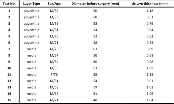
TABLE 1. Demographic information for the collected ATAA specimens.
Test No. Layer Type Sex/Age Diameter before surgery (mm) Ex vivo thickness (mm)
1 adventitia M/67 50 1.18 2 adventitia M/36 50 0.51 3 adventitia M/55 53 0.79 4 adventitia M/81 54 0.64 5 adventitia M/76 52 0.62 6 adventitia M/71 48 0.55 7 media M/70 63 0.89 8 media M/67 50 0.68 9 media M/54 60 0.98 10 media M/55 53 1.09 11 media F/76 55 1.15 12 media M/81 54 0.91 13 media M/68 59 1.02 14 media M/69 51 1.09 15 media M/71 48 1.04
TABLE 2. Components of the Cauchy stress tensor reported at the NodeMAX, NodeTOP and NodeRUP locations (in MPa). Test No. 1 to 6 were adventitia layers and Test No. 7 to 15 were
media layers.
NodeMAX NodeTOP NodeRUP
Test No.
σ
11σ
22σ
12σ
11σ
22σ
12σ
11σ
22σ
12 1 1.124 1.091 -0.036 0.681 0.842 -0.098 1.128 1.062 -0.005 2 3.066 3.812 -0.065 3.035 3.778 -0.064 2.954 3.527 0.084 3 1.233 1.613 -0.011 1.246 1.554 0.023 0.977 0.949 0.189 4 0.938 0.853 0.001 0.922 0.863 -0.002 0.922 0.795 0.012 5 1.964 1.642 0.050 1.920 1.647 0.020 1.699 1.419 -0.042 6 1.035 1.019 -0.046 1.035 1.019 -0.046 0.920 0.933 -0.108 7 0.756 0.997 0.041 0.677 0.909 0.078 0.640 0.924 0.006 8 1.764 1.654 0.097 1.617 1.573 0.077 1.120 0.913 -0.051 9 1.042 1.064 -0.06 1.033 1.067 -0.05 0.903 1.049 -0.027 10 1.308 1.007 -0.012 1.042 1.038 -0.028 1.174 0.927 -0.042 11 0.627 0.622 -0.009 0.549 0.602 -0.03 0.552 0.605 -0.025 12 0.631 0.630 0.076 0.664 0.633 0.042 0.655 0.626 0.040 13 0.819 0.720 -0.055 0.805 0.714 -0.053 0.815 0.725 -0.051 14 0.728 0.866 -0.018 0.800 0.858 -0.016 0.791 0.805 0.0001 15 0.805 0.601 -0.037 0.79 0.588 -0.044 0.714 0.546 -0.041 Mean 1.18 1.21 -0.006 1.12 1.17 -0.013 1.06 1.05 -0.004 Std. 0.64 0.80 0.05 0.64 0.79 0.05 0.59 0.71 0.06TABLE 3. Comparison between four different ultimate stress values calculated at different locations within the same tissue. Test No. 1 to 6 were adventitia layers and Test No. 7 to 15 were
media layers.
Test No. (MPa) (MPa) (MPa) (MPa)
1 0.9695 1.1481 0.8889 1.0719 2 3.5825 3.8183 3.7841 3.5269 3 1.1725 1.6134 1.5558 0.9755 4 0.8116 0.9385 0.9222 0.8265 5 1.5928 1.9724 1.9221 1.4644 6 0.8414 1.0752 1.0752 0.9335 7 0.7275 1.0049 0.9337 0.6412 8 1.4016 1.8214 1.6756 1.0057 9 0.8503 1.1148 1.1036 0.9309 10 0.8215 1.3086 1.0692 1.1733 11 0.4863 0.6346 0.6169 0.6015 12 0.5559 0.7074 0.6936 0.6286 13 0.7283 0.8438 0.8302 0.7259 14 0.8244 0.8687 0.8623 0.8028 15 0.6386 0.8121 0.7994 0.5891 Mean 1.0669 1.3121 1.2488 1.0598 Std. 0.7573 0.7979 0.7933 0.7236
Fig. 2. View of the experimental set-up and the inflation of the ATAA layer through the left and right cameras of the DIS-C system. An image is recorded every loading stage defined at 3 kPa, for the duration of the test. Note that the acrylic protector is used to prevent water from reaching the
Fig. 3. Reconstructed shape of the ATAA layer at the final inflation stage. The 3D coordinates of each material point were used to reconstruct the shape.
Fig. 5. Discretization of the surface. The unchanged mesh is deformed from a) the initial to b) the current configuration. For one boundary element the local ( , , ) Cartesian frame used to define
Fig. 6. Top view of the element by element comparison between stress fields calculated by a) the FEA simulation (reference) and b) our approach. The absolute error (in MPa) between a) and b) is
Fig. 7. The a) stress field ( ), b) displacement field ( ) and c) strain field ( ) for three ATAA specimens all at a pressure of 0.027 MPa.
Fig. 8. ATAA rupture. For each test, a) the color map of the thickness measurement, b) the deformed mesh ( = NodeMAX, = NodeTOP, = NodeRUP) and c) the rupture picture where
Fig. 9. Four different ultimate stresses for each of the 15 ATAA samples where is the Laplace stress calculated from Eq. (12), is the maximum principal stress, is the maximum principal stress at the node of the top, and is the rupture stress calculated from Eq. (10).
Fig. 10. Local thickness evolution (Eq. (11)) in mm. for one representative ATAA sample (Test No. 14). Top view from the initial stage (0.003 MPa) until the final stage (0.057 MPa) and the image
APPENDIX A
1To validate the membrane assumption the stress fields calculated by our approach on a pre-defined
2
geometry were compared to reference stresses provided by a finite element analysis (FEA) on the
3
same reference geometry. In order to compare exactly the data at the same points, we used the
4
same nodal arrangement for both methods, which means that we had to interpolate the reference
5
FEA results into our own predefined mesh used in our approach (644 nodes and 1203 elements).
6 7 8 Validation Process 9 10
A FEA simulation of the inflation process was performed with the aim to numerically reproduce an
11
experimental dataset. Using the Abaqus® software we created a 0.85 mm thick circular patch of 30
12
mm of diameter, corresponding to the area of interest (AOI) for an inflated of the experimental aortic
13
layers. In order to perform the numerical simulation it was necessary to define the material
14
properties of the circular patch, which were based on the anisotropic hyperelastic
Holzapfel-Gasser-15
Ogden (HGO) model (Holzapfel et al. 2000). The material properties defined for the FEA simulation
16
were obtained from the literature: density= 5.0e-4 , C10= 0.0764 MPa, D= 1.e-8 , k1= 0.0839611 MPa,
17
k2= 1.2644611 , κ= 0 and β= 41 °.
18 19
The nodes on the boundary of the circular patch were pinned allowing their rotation. The applied
20
load was defined as a uniform pressure of 0.06 MPa, applied to the inner surface of the circular patch
21
(Fig. A1). Finally the mesh size of the simulation was defined by 10119 nodes and 19887 shell
22
elements.
23 24
25
The FEA simulation provided the displacement and stress distributions at the end of the inflation. The
26
stress fields provided by this FEA simulation were then used as a reference for the validation of our
27
approach and the final geometry provided by this FEA was also used as the reference geometry for
28
validating our approach.
29 30
For our simulation, we used shell elements which yielded two sets of stress fields in the results, one
31
located at the inner surface (Fig. A2-a) and another located at the outer surface (Fig. A2-b) of the
32
inflated membrane. The stress at the inner surface was slightly lower than the stress at mid-thickness
33
and the stress at the outer surface was slightly higher than the stress at mid-thickness. For a 0.85 mm
34
thick sheet, it was estimated that the mean absolute difference between the stress at the inner and
35
outer surface was 0.32 MPa for σ , 0.26 MPa for σ and 0.0013 MPa for σ . In contrast, our
36
approach provides directly the stress field at mid-thickness. Knowing this, the two stress fields, outer
37
and inner, obtained from the FEA simulation were averaged to provide an accurate comparison with
38
our approach.
39 40
Fig. A1. Lateral view of the circular patch created in Abaqus® software. Boundary conditions allow the rotation. A uniform pressure is applied to the inner surface of the patch.
41
After extracting the nodal displacements, we interpolated the values across a grid of pixels in order
42
to create a dataset with the same spatial resolution as the experimental data (Fig. A3). Then we
43
applied our approach to these experimental-like data in order to reconstruct the maps of the Cauchy
44
stress tensor. Using the Abaqus® output file, we interpolated the stress values at the same nodes
45
that we reconstructed them. Afterwards our Cauchy stress estimates, from applying our approach to
46
the experiment-like data, were compared to the Cauchy stress values provided by the FEA
47
computation.
48
49
Fig. A2. FEA computation (Abaqus® software top view) provided stress fields located at a) the inner surface and b) the outer surface of the inflated membrane.
50
Therefore, we were able to compare, element by element, the results of our approach and those of a
51
reference FEA simulation. In Figure A4-a the reference stress distribution from the FEA simulation is
52
shown and in Figure A4-b the stress distribution from our approach is displayed. The difference
53
between both was calculated at each element and is presented in Figure A4-c. Mean absolute errors
54
of 0.031 MPa for , 0.002 MPa for , and 0.005 MPa for .were calculated between our
55
approach and the FEA simulation. These mean absolute errors are equivalent to mean relative errors
56
of 3.5% for , 0.3% for and 0.5% for . 57
58
Fig. A3. The 3D deformed geometry (surface) obtained with the FEA simulation (blue) was imported into Matlab®
a) Nodes where the Cauchy stress will be estimated are defined (red dots) across this surface b) The surface is meshed using the Delaunay triangulation.
59
The differences in the results are due to the different boundary conditions used for each method (i.e.
60
pinned for the FEA approach and traction boundary conditions for our approach). An interesting
61
result was that the boundary conditions only affected the estimated stress near the border. After
62
removing the three first stripes of triangles adjacent to the border (Fig. A4-d), the mean absolute
63
errors were reduced to 0.008 MPa for , 0.013 MPa for , and 0.008 MPa for . These mean
64
absolute errors are equivalent mean relative values of 0.8% for , 1.4% for and 0.8% for ,
65
indicating that the stress estimates contain some errors along the border due to the assumed
66
Fig. A4. Top view of the element by element comparison between stress fields calculated by a) the FEA simulation (reference) and b) our approach. The absolute error (in MPa) between a) and b) is
boundary conditions but these errors vanish rapidly away from the border.