HAL Id: hal-00462786
https://hal.archives-ouvertes.fr/hal-00462786
Submitted on 10 Mar 2010
HAL is a multi-disciplinary open access
archive for the deposit and dissemination of
sci-entific research documents, whether they are
pub-lished or not. The documents may come from
teaching and research institutions in France or
abroad, or from public or private research centers.
L’archive ouverte pluridisciplinaire HAL, est
destinée au dépôt et à la diffusion de documents
scientifiques de niveau recherche, publiés ou non,
émanant des établissements d’enseignement et de
recherche français ou étrangers, des laboratoires
publics ou privés.
Some Interval Approximation Techniques for MINLP
Nicolas Berger, Laurent Granvilliers
To cite this version:
Nicolas Berger, Laurent Granvilliers. Some Interval Approximation Techniques for MINLP. SARA
2009: The Eighth Symposium on Abstraction, Reformulation and Approximation, Jul 2009, Lake
Arrowhead, California, United States. pp.26-33. �hal-00462786�
Some Interval Approximation Techniques for MINLP
Nicolas Berger and Laurent Granvilliers
Universit´e de Nantes – CNRS – France
2, rue de la Houssini`ere – BP 92208 – F-44322 Nantes Cedex 3 nicolas.berger, [email protected]
Abstract
MINLP problems are hard constrained optimization problems, with nonlinear constraints and mixed dis-crete continuous variables. They can be solved using a Branch-and-Bound scheme combining several methods, such as linear programming, interval analysis, and cut-ting methods. Our goal is to integrate constraint pro-gramming techniques in this framework. Firstly, global constraints can be introduced to reformulate MINLP problems thus leading to clean models and more precise computations. Secondly, interval-based approximation techniques for nonlinear constraints can be improved by taking into account the integrality of variables early. These methods have been implemented in an interval solver and we present experimental results from a set of MINLP instances.
Introduction
Mixed Integer Nonlinear Programming (MINLP) prob-lems are constrained optimization probprob-lems with both discrete and continuous variables, where the objective function may be nonconvex, and the constraints may be nonlinear (Grossmann 2002; Tawarmalani & Sahinidis 2004). They can be found in many application domains such as engineering design, computational biology, and portfolio optimization.
The integrality of variables and the nonconvexity of functions make MINLP problems difficult to solve. The general Branch-and-Bound scheme is a method of choice, provided bound constraints on the variables. The main principle is to divide the initial problem into a set of subproblems by enumerating discrete domains or bisecting continuous domains. Bounding techniques are used to compute lower and upper bounds on the objective function, thus allowing the rejection of sub-problems proved to be non optimal.
Two kinds of bounding techniques may be combined. Interval methods (Moore 1966) can derive improved bounds on domains from relaxed NLP problems, lo-cally considering discrete variables as continuous. Up-per bounds on the objective function can also be calcu-lated, possibly using a local optimizer to find feasible Copyright c 2009, Association for the Advancement of Ar-tificial Intelligence (www.aaai.org). All rights reserved.
points (Neumaier 2004). Linear methods can compute global optima over relaxed LP problems, requiring non-linearities to be reformulated and linearized (Sherali & Adams 1999). This way, lower bounds on the objective function can be obtained. It turns out that these tech-niques complement each other. Reducing the domain bounds leads to tighter linear relaxations, and then to more precise lower bounds. Several solvers integrate these techniques, such as Couenne (Belotti et al. 2008), which is part of the COIN-OR infrastructure.
We focus on improving state-of-the-art interval-based bounding techniques for MINLP problems. Our start-ing point is the interval constraint propagation frame-work (Cleary 1987; Lhomme 1993; Van Hentenryck, Michel, & Deville 1997). Constraint propagation is a general bounding algorithm where contracting op-erators are applied on domains until they are not re-fined enough. These operators are based on interval arithmetic, numerical methods for differentiable prob-lems, and projection techniques to tackle nonlinear con-straints. They require functions and constraints to be expressed as combinations of arithmetic operations and elementary functions.
In this paper, we propose two kinds of improve-ments. Firstly, the integrality constraints can be taken into account during constraint propagation to reinforce domain contractions, as done by Apt and Zoeteweij (Apt & Zoeteweij 2007) for pure integer prob-lems. Secondly, MINLP problems may be reformulated by means of so-called global constraints such as the fa-mous alldifferent constraint stating that a set of in-teger variables must all have different values. These constraints give a better expressiveness at modeling time. Moreover, they are associated with specialized domain contraction algorithms. In fact, we investigate the well-known approach of mixing constraints and op-timization techniques (Hooker 2007) for MINLP prob-lems.
The remaining of this paper is organized as follows. The following section introduces MINLP problems. Re-formulations using global constraints are illustrated for two non trivial problems. Interval approximation tech-niques and proposed improvements are described in the third section. The next section reviews several ways of
processing the alldifferent constraint. An experi-mental study and a conclusion follow.
MINLP and Reformulations
The notion of MINLP problem is introduced in this section and we show how to reformulate two real-world problems using the alldifferent global constraint.
Definition
Consider the MINLP problem min
x∈Ωf (x)
such that Ω is the feasible region defined by (P) gj(x) = 0 ∀j ∈ J
xl
i6xi6xui ∀i ∈ I
xk∈ Z ∀k ∈ K ⊆ I
where f and the gj are possibly nonconvex functions
and x is the vector of variables such that the xk are
integer variables for all k ∈ K. The goal is to find the feasible points x minimizing f .
Example 1 Consider the constraint x2− x21+ 1 = 0
and let the objective be min(x2+1.1(x1−1)). Solving the
first-order optimality conditions leads to the global min-imum (−0.55, −0.6975) with objective −2.4025 (white point).
Now suppose that x is an integer variable. The global minimum becomes (−1, 0) with objective −2.2 (black point).
b
c
b
Considering integrality constraints make problems more complex to solve. In particular, the optimality conditions do not hold at local optima.
Reformulations
We first introduce Montemanni’s mixed-integer pro-gramming formulation for the total flow time single machine robust scheduling with interval data (Monte-manni 2007), where an interval of equally possible pro-cessing times is considered for each job. Optimization is carried out according to a robustness criterion: we want to find the schedule that performs the best under the worst case scenario.
Each of some N tasks must be assigned a distinct processing order, which models in MINLP using binary variables: xik is true when task i is processed in kth
position under the constraints that each job is given exactly one position and each position is given to ex-actly one job:
N X i=1 xik= 1, N X k=1 xik= 1.
This scheme perfectly fits with the purpose of the alldifferent global constraint. Given a set of inte-ger variables ti ranging in {1, . . . , N}, the two above
constraints can be reformulated into an alldifferent global constraint:
alldifferent([t1, . . . , tN]).
The model we give here for the robust scheduling problem results from a well-known technique that ex-ploits the unimodularity property of the nested maxi-mization problem. min N X i=1 ηi+ N X k=1 τk subject to : (1) alldifferent(t1, . . . , tN), (2) ti = N X k=1 xi,k· k, (3) N X k=1 xik = 1, (4) ηi+ τk > pi k X j=1 (k − j)xij + pi N X j=k (k − j)xij, xik ∈ {0, 1}, ti ∈ {1, . . . , N}, ηi ∈ R, τk ∈ R.
Constraint (1) expresses that each task must have a distinct processing order; (2) channels this value to binary variables as needed by constraint (4). Con-straint (3) forbids this channeling to imply more than one binary variable set to true. Finally, (4) simply links the variables we maximize the sum of with the arithmetic expression of the regret cost of the worst case scenario for this schedule.
We now introduce a part of the simplified yet realis-tic model for the nuclear reactor core optimal reload pattern problem (Quist et al. 1999) that can be found in the MINLPLib collection of MINLP prob-lems (Bussieck, Drud, & Meeraus 2003).
The nuclear reactor reloading problem consists in finding the optimal fuel reloading pattern for a nuclear
reactor core. In the model we consider here, the ob-jective is to maximize the end-of-cycle ratio of neutron production rate over neutron loss rate —what is called the reactivity of the core— while satisfying some secu-rity constraints, given that the position of fuel bundles at the end of a cycle determines their initial properties for the next cycle.
The trajectory of the bundles in the core from cycle to cycle can be represented by a matrix of the following kind:
4 → 7 → 3 → 1
2 → 8 → 10 → 12
5 → 11 → 6 → 9
We see here a possible 4 cycles long trajectory, for a core of 12 nodes in which 3 bundles —a quarter of the bundles— are discharged at each end-of-cycle. Each number refers to a different node of the core. According to this matrix, the bundles located at nodes 1, 12 and 9 are discharged at each reloading while fresh bundles are inserted into nodes 4, 2 and 5. The bundle in node 7 is moved to node 3, the bundle in node 10 is moved to node 12, etc.
Here again, the classical MINLP approach to model-ing the assignment of a node to a cell of the matrix is to use binary variables: xi,l,m is true when the bundle in
node i is affected to column l and row m in the trajec-tory matrix. We then have to constrain these variables so as exactly one will be set to true for a given i —each node must appear exactly once in the matrix. Recip-rocally, exactly one variable must be set to true for a given position l, m in the matrix, as each cell of the matrix must be assigned to exactly one node. Thus we have: N X i=1 xi,l,m= 1, L X l=1 M X m=1 xi,l,m= 1.
It turns out that the problem of assigning each node a position in the trajectory matrix can be expressed by means of the alldifferent global constraint. Given the following indexing of the cells:
1 2 3 4
5 6 7 8
9 10 11 12
each node i must be assigned a distinct position num-ber ni, ranging in {1, . . . , 12}, which fits perfectly with
the purpose of this global constraint. Then the tra-jectory matrix assignment constraint models simply as following:
alldifferent([n1, . . . , nN]).
Interval Approximation Techniques
Interval constraint propagation can be applied on NLP problems defined from MINLP problems by relaxing the integrality constraints. Some interval solvers are able
to tackle these constraints by regularly truncating the bounds of integer domains. In this section, we propose to take them into account in the early phases of interval calculations, leading to stronger domain contractions.
Interval arithmetic
Interval arithmetic is an arithmetic over real intervals. For instance we have:
[a, b] + [c, d] = [a + c, b + d] [a, b] − [c, d] = [a − d, b − c] [a, b]3 = [a3, b3]
These operations can be used to enclose the range of a real function over an interval domain (Moore 1966). For instance, let f (x) = x3
+1 and let x ∈ Dx= [−2, 2].
Then we have:
f (x) ∈ F (Dx) = Dx3+ [1, 1] := [−7, 9]
where F is an interval extension of f .
Constraint propagation
Interval arithmetic can be used to implement contract-ing operators of domains of variables occurrcontract-ing in linear or nonlinear constraints. For instance let x+y = 1 with x ∈ [0, 2] and y ∈ [0, 2]. It is immediate to rewrite the constraint as x = f (y) = 1 − y. Then the domain of x can be contracted as follows:
Dx := hull(Dx∩ F (Dy)) := [0, 1]
where hull computes the interval enclosure of a set of real numbers. This operation is necessary in some cases, when F results in a union of intervals, as we will see later.
This operator computes the projection of constraint x + y = 1 over x within the given interval domain using a constraint inversion method. A very similar opera-tor can be associated to the projection over y. This idea originates from (Cleary 1987) and it has been ex-tended to efficiently cope with arbitrary complex con-straints (Benhamou et al. 1999).
Given a constraint system, a set of contracting oper-ators can be defined from the set of constraint projec-tions. They have to be iteratively applied to reach a stable state where no domain can be reduced enough, in a so-called constraint propagation algorithm.
Handling integrality constraints
As said before, some interval solvers are able to apply integrality constraints during constraint propagation. The common way consists in implementing, for every integer variable x, a contracting operator truncating the domain bounds, as follows:
Dx:= hull(int(Dx))
where int takes the integral part of a set of real numbers. This operator is regularly applied during constraint propagation, allowing to maintain integer bounds for the integer variables. In fact, it is possible to perform truncation directly in contracting operators (next para-graph) and to improve interval arithmetic to cope with integer data (last paragraph).
Early truncation Let x = f (y) be a projection con-straint and let x be an integer variable. Then the do-main of x can be reduced as follows:
Dx← hull(int(Dx∩ F (Dy))) (1)
where the integral part of the set Dx∩ F (Dy) happens
before the hull. This operator may replace the classi-cal implementation of integrality constraints, which is equivalent to:
Dx := hull(Dx∩ F (Dy))
Dx := hull(int(Dx)) (2)
where the processing of the integrality constraint is done after the domain contraction wrt. the constraint.
We have the following proposition. Proposition 1 Let D1
x be obtained from equation (1)
and let D2
xbe obtained from equation (2). Then we have
D1 x⊆ Dx2.
As a consequence, every contracting operator for the domain of an integer variable must compute integral sets before returning interval hulls.
Example 2 Let y = x2 such that y ∈ [2, 3] is a real
variable and x ∈ [−2, 2] is an integer variable. The domain of x is computed by means of the inverse of the square operation applied on y. It follows that x must belong to [−√3, −√2] ∪ [√2,√3]. Then we have:
hull(int(hull([−√3, −√2] ∪ [√2,√3])) = [−1, 1] hull(int([−√3, −√2] ∪ [√2,√3]) = ∅
which shows that the integrality constraint must be con-sidered as soon as possible during interval computa-tions.
Improved arithmetic Interval arithmetic can be improved by means of integrality constraints. For in-stance, let x be an integer variable and suppose that Dx strictly contains 0. Then we have:
1/x ∈ [−1, 1/ min(Dx)] ∪ [1/ max(Dx), 1] (3)
This new operation may be compared with the original definition of the division when the integrality constraint is relaxed, as follows:
1/x ∈ [−∞, 1/ min(Dx)] ∪ [1/ max(Dx), +∞] (4)
It is clear that equation (3) leads to a more pre-cise interval wrt. equation (4), by tightening the ex-tremal bounds. In fact, there is no real number within [−∞, −1) ∪ (1, +∞] obtained as 1/x with x integer.
The purpose here is not to present the full interval arithmetic extended to mixed-integer problems. How-ever, let us remark that the division is much useful, in particular for polynomial problems, as illustrated in the following example.
Example 3 Let x ∈ [−10, 10] be an integer variable
and let y ∈ [−10, 10] be a real variable. Consider the system xy = 1, x + y = 2.
1. By using Algorithm (4) of the interval division the first equation becomes useless. Only the second equa-tion is useful to contract the domains, as follows:
Dx := hull(Dx∩ (2 − Dy)) := [−8, 10]
Dy := hull(Dy∩ (2 − Dx)) := [−8, 10]
2. Considering now the integrality of x, Algorithm (3) can be enforced. As a consequence, the first equa-tion leads to contract the domain of y and to prop-agate through the system, eventually computing the only solution, as follows:
Dy := hull(Dy∩ (1/Dx)) := [−1, 1]
Dx := hull(int(Dx∩ (2 − Dy))) := [1, 3]
Dy := hull(Dy∩ (1/Dx)) := [13, 1]
Dx := hull(int(Dx∩ (2 − Dy))) := 1
Dy := hull(Dy∩ (1/Dx)) := 1
Taking integrality of variables into account early dur-ing arithmetic evaluation not only leads to stronger domain reductions as shown above, but also can help achieving exponential solving time gains.
Example 4 Let x be an n-dimensional real vector and let y be an n-dimensional integer vector. Suppose that each variable lies in [−108, 108] and consider the
follow-ing system: xiyi = 1, i = 1, . . . , n n X i=1 x2i = 2n
If Alg. (3) is implemented then the constraint propaga-tion algorithm alone is able to prove inconsistency. The new division method allows domains to be contracted with respect to the constraint xiyi= 1.
Only weak contractions are obtained by means of Alg. (4). To prove inconsistency, constraint propaga-tion must be combined with a bisecpropaga-tion technique. How-ever, it requires an exponential number of bisections, exactly 2n−1.
Example 5 Let x be a n-dimensional real vector and let y be a n-dimensional integer vector. Suppose that each variable lies in [−108, 108] and consider the
fol-lowing system: (xi− 1)yi = 1, i = 1, . . . , n log( n Y i=1 yi) = 1
The following table shows the number of bisections re-quired to prove inconsistency, using the two different algorithms of the division.
n Alg. (3) Alg. (4) Ratio
3 7 16 2.3 4 23 71 3.1 5 63 288 4.6 6 159 1099 6.9 7 383 4016 10.5 8 895 14223 15.9 9 2047 49216 24.0
Once again, the new algorithm is shown to be more ef-ficient. We obtain an exponential gain in the number of bisections, where the ratio can be expressed as the function f (n) = 1.4n.
Processing Global Constraints
In this section, we present several ways of processing the alldifferentconstraint, either transforming it into a set of constraints supported by the solver, or imple-menting specialized algorithms.
Techniques
Clique of disequalities A naive implementation of the alldifferent constraint for n variables uses a clique of disequalities on pairs of variables, thereby adding in the background O(n2) new constraints to the
model. Many opportunities for filtering the domains of the variables are lost during such a translation; on the other hand, it only requires that the solver provides a disequality constraint.
Inter-distance constraints When the solver does not implement a disequality constraint, we can model each disequality between two integer variables as a greater or equal to one distance constraint:
{|xi− xj| > 1 | 1 6 i < j 6 n}.
where the absolute can also be replaced with a square (xi− xj)2. This way, we still have the ability to express
some model making use of the alldifferent constraint in a solver that does not implement a disequality con-straint.
Sum constraint We can strengthen the clique mod-elind above with the help of the convex hull relaxation of the alldifferent constraint as defined in (Hooker 2002) for integer interval domains:
n X j=1 xj = n(n + 1) 2 X j∈J xj >|J|(|J| + 1) 2 , ∀J ⊂ {1, . . . , n} with |J| < n provided that xj ∈ [1, n]. If we have xj ∈ [a, b] with
a 6= 1, it suffices to consider the translation yj = xj−
a + 1 ∈ [1, b − a + 1].
However, the number of constraints in the relaxation constraints set described by the formula above grows exponentially with the number of variables in use in the model, and it easily becomes impractical to use this set as is. Still, our experiments showed that the fastest minimal subset of the convex hull relaxation was the one consisting only of the equality constraint summing all variables.
Domain cardinality We introduce here a domain cardinality operator # applying on a union of integer intervals and returning the number of distinct values in
it. Now suppose that a alldifferent constraint on a set of variables x1, . . . , xn holds true. Then we have
# (Dx1∪ · · · ∪ Dxn) > n
where Dxi is the domain of xi for every i. This is in
fact the well-known necessary condition based on the Hall interval associated with the whole set of variables. The following specialized algorithm is implemented. First, if the domain cardinality operator calculates an integer smaller than n then the constraint fails. Sec-ond, when a variable is fixed to some value, this value is removed from the domains of all the other variables for which it is a bound value. This later technique cor-responds to the classical processing of disequality con-straints: given x 6= y and x = a then remove a from the domain of y.
Bound consistency We can also implement a ded-icated, state-of-the-art bound consistency filtering al-gorithm such as the one given in (L´opez-Ortiz et al. 2003).
Experiments
In this section are presented our experimental results on both generated and real-world problems.
Academic problems We designed three problems with different features. The first one int-frac is a purely discrete problem:
alldifferent(x1, . . . , xn), x1 x2 + . . . + xn−1 xn =1 2 + . . . + n − 1 n , xi+ 1 6 xi+2, 1 6 i 6 n, i odd, xi∈ {1, . . . , n}, 1 6 i 6 n.
The second one mixed-sin is a mixed-integer prob-lem with linear and non-linear constraints:
alldifferent(p1, . . . , pn), xipi + X j6=i xj= i, 1 6 i 6 n, sin(πxi) = 0, 1 6 i 6 n, pi∈ {1, . . . , n}, 1 6 i 6 n, xi∈ [−100, 100], 1 6 i 6 n.
The third one hard-mixed-sin is a mixed-integer problem generator inspired from mixed-sin but with harder non-linear constraints:
alldifferent(p1, . . . , pn), sin(xipi) + X j6=i xj= i, 1 6 i 6 n, sin(πxi) = 0, 1 6 i 6 n, pi∈ {1, . . . , n}, 1 6 i 6 n, xi∈ [−10, 10], 1 6 i 6 n.
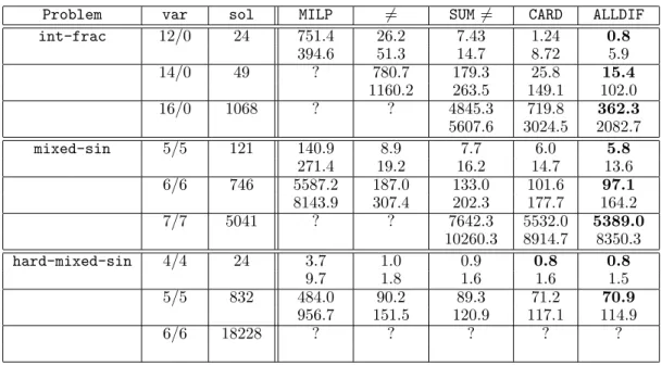
The experimental results are presented in Table 1. All the experiments were conducted on an Intel Xeon at 3 GHz with 16 GB of RAM, using the interval solver Realpaver 1.0 (Granvilliers & Benhamou 2006). For
every problem, var gives the number of discrete vari-ables and the number of continuous varivari-ables on the constraint model with alldifferent constraints and solstands for the number of solutions. The last four columns correspond to the different methods: MILP for the MILP problem formulation; 6= for the problem for-mulation with disequality constraints; SUM 6= for the problem formulation with disequality constraints and the convex hull relaxation; CARD for the problem for-mulation with cardinality constraints; ALLDIF for the problem formulation with the dedicated, state-of-the-art alldifferent global constraint filtering. The solv-ing times in seconds are given in the first row and the number of branching steps in thousands are given in the second row. A question mark stands for a method that cannot solve the problem in reasonable time.
First of all, it is clear that the MILP formulation is not efficient for those problems. For instance, let us consider the constraint b +P
ibi = 1 stating that
exactly one variable among a set of Boolean variables must be true —this is one of the Boolean constraints used to simulate the alldifferent constraint. Suppose that the domain of b is split. If b = 1 it is immediate to derive that each bi is equal to 0. However, if b = 0
nothing can be deduced for the other variables. That may explain the great number of splitting steps in the MILPcolumn.
The 6= formulation is more efficient than the MILP formulation but only for small problem instances: in case of larger problems, it does not permit to solve the problem in reasonable time. On the contrary, the SUM 6= formulation is able to solve all the instances in a significantly lower time. However, we can see that the harder the problem, the smaller the improvement wrt. the 6= formulation.
The CARD formulation is up to five times faster than the SUM 6= formulation, especially on instances of int-fracwhile in other cases, solving times are only re-duced in a factor up to a third. The ALLDIF formulation performs as good as CARD on instances of mixed-sin and hard-mixed-sin, but is a bit less than twice faster on instances of int-frac.
Real-world problems We solved several instances of the problems we described in Section 2: three of Scheduling with respectively 9, 10, 11 tasks; two of Nuclear, one with a trajectory matrix of size 3x3 with each cycle divided into 3 time steps —NuclearA— and one with a trajectory matrix of size 4x3 with each cy-cle divided into 2 time steps —Nucy-clearB. Experimental settings are the same than introduced in the previous subsection and the results are presented in Table 2.
The CARD formulation is always the fastest. Nonethe-less, for those instances the 6= formulation remains com-petitive which was clearly not the case for the generated problems in the previous subsection. An explanation for this can be that in these real-world problems, the alldifferent constraint yields not many domain re-ductions wrt. the other hard, many continuous
con-straints. In such a situation, the simpler the filtering, the faster the resolution. This should also explain that the MILP formulation for Nuclear instances surprisingly performs quite as well as the best formulation.
Another surprising result is the behavior of the ALLDIF formulation for all the tested instances. The MILP formulation on Schedule instances excepted, it is always slightly slower than the other formulations. An explanation could be that the dedicated filtering algorithm does not yield sufficiently many domain re-ductions wrt. its time cost, which makes the other for-mulations competitive.
To conclude, it seems that the CARD formulation is a good approach to implement the alldifferent con-straint in continuous concon-straint solvers. Its imple-mentation, which simply requires to compute domain unions and to remove values at domain bounds, is very easy. Furthermore, the resulting domain contractions can be much better than the other formulations.
Conclusion
Interval methods are designed to solve NLP problems using a branch-and-bound algorithm. In this paper, we have proposed several improvements for solving MINLP problems. We have shown that interval arithmetic can be extended to process problems with discrete and con-tinuous variables. The new operations handle the inte-grality constraints, resulting in tighter interval compu-tations for mixed nonlinear expressions.
We have also proposed to reformulate combinato-rial parts of MINLP problems using global constraints. Stronger domain contractions are obtained by means of specialized algorithms for processing these global straints. Several algorithms for the alldifferent con-straint have been compared. It reveals that simple tech-niques (MILP models and sum relaxations) are enough for small integer subproblems. However, bound consis-tency algorithms behave better in general. We believe that they must be implemented in efficient mixed con-straint solvers.
The next step will be to fully implement a mixed interval solver and to integrate it in a MINLP solver like Couenne.
Acknowledgments
We are grateful to Fr´ed´eric Goualard for interesting dis-cussions on these topics.
References
Apt, K., and Zoeteweij, P. 2007. An Analysis of Arith-metic Constraints on Integer Intervals. Constraints 12(4):429–468.
Belotti, P.; Lee, J.; Liberti, L.; Margot, F.; and Wacher, A. 2008. Branching and Bounds Tightening Techniques for Nonconvex MINLP. Submitted. Benhamou, F.; Goualard, F.; Granvilliers, L.; and Puget, J. 1999. Revising Hull and Box Consistency. In ICLP.
Bussieck, M. R.; Drud, A. S.; and Meeraus, A. 2003. Minlplib - a collection of test models for mixed-integer nonlinear programming. INFORMS Journal on
Com-puting 15(1).
Cleary, J. 1987. Logical Arithmetic. Future Computing
Systems 2(2):125–149.
Granvilliers, L., and Benhamou, F. 2006. Algorithm 852: Realpaver: an interval solver using constraint satisfaction techniques. ACM Trans. Math. Softw.
32(1):138–156.
Grossmann, I. 2002. Review of Nonlinear and Mixed Integer and Disjunctive Programming Techniques.
Op-timization and Engineering 3(3):227–252.
Hooker, J. N. 2002. Logic, optimization and con-straint programming. INFORMS Journal on
Comput-ing 14:295–321.
Hooker, J. 2007. A Framework for Integrating Opti-mization and Constraint Programming. In SARA. Lhomme, O. 1993. Consistency Techniques for Nu-meric CSPs. In IJCAI.
L´opez-Ortiz, A.; Quimper, C.-G.; Tromp, J.; and van Beek, P. 2003. A fast and simple algorithm for bounds consistency of the alldifferent constraint. In IJCAI. Montemanni, R. 2007. A Mixed Integer Program-ming Formulation for the Total Flow Time Single Ma-chine Robust Scheduling Problem with Interval Data.
Journal of Mathematical Modelling and Algorithms
6(2):287–296.
Moore, R. 1966. Interval Analysis. NJ: Prentice-Hall, Englewood Cliffs.
Neumaier, A. 1990. Interval methods for systems of equations. In Encyclopedia of Mathematics and its
Ap-plications, volume 37. Cambridge Univ. Press,
Cam-bridge.
Neumaier, A. 2004. Complete Search in Continu-ous Global Optimization and Constraint Satisfaction.
Acta Numerica 13:271–369.
Quist, A.; Geemert, R. V.; Hoogenboom, J.; Illest, T.; Klerk, E. D.; Roos, C.; and Terkaly, T. 1999. Finding Optimal Nuclear Reactor Core Reload Patterns Using Nonlinear Optimization and Search Heuristics.
Engi-neering Optimization 32(2):143–176.
Sherali, H., and Adams, W. 1999. A
Reformulation-Linearization Technique for Solving Discrete and Con-tinuous Nonconvex Problems. Kluwer Academic
Pub-lishers.
Tawarmalani, M., and Sahinidis, N. 2004. Global Optimization of Mixed Integer Nonlinear Programs: A Theoretical and Computational Study. Mathematical
Programming 99(3):563–591.
Van Hentenryck, P.; Michel, L.; and Deville, Y. 1997.
Numerica: a Modeling Language for Global Optimiza-tion. MIT Press.
Problem var sol MILP 6= SUM6= CARD ALLDIF int-frac 12/0 24 751.4 26.2 7.43 1.24 0.8 394.6 51.3 14.7 8.72 5.9 14/0 49 ? 780.7 179.3 25.8 15.4 1160.2 263.5 149.1 102.0 16/0 1068 ? ? 4845.3 719.8 362.3 5607.6 3024.5 2082.7 mixed-sin 5/5 121 140.9 8.9 7.7 6.0 5.8 271.4 19.2 16.2 14.7 13.6 6/6 746 5587.2 187.0 133.0 101.6 97.1 8143.9 307.4 202.3 177.7 164.2 7/7 5041 ? ? 7642.3 5532.0 5389.0 10260.3 8914.7 8350.3 hard-mixed-sin 4/4 24 3.7 1.0 0.9 0.8 0.8 9.7 1.8 1.6 1.6 1.5 5/5 832 484.0 90.2 89.3 71.2 70.9 956.7 151.5 120.9 117.1 114.9 6/6 18228 ? ? ? ? ?
Table 1: Solving time in seconds (first row) and number of branchings in thousands.
Problem var sol MILP 6= SUM6= CARD ALLDIF Schedule9 90/19 1 750.3 9.0 8.5 8.0 9.8 169.7 1.9 1.9 1.9 1.9 Schedule10 110/21 1 1 303.9 38.0 38.5 35.2 37.9 229.0 6.6 6.6 6.6 6.6 Schedule11 132/23 1 ? 205.0 197.6 186.3 228.6 25.5 25.5 25.5 25.5 NuclearA 90/57 1 78.7 79.2 79.0 78.0 81.0 6.4 6.4 6.4 6.4 6.4 NuclearB 156/50 1 659.7 660.8 671.3 658.2 693.0 12.7 12.7 12.7 12.7 12.7