Kinetostatic Performance of a Planar Parallel Mechanism with Variable Actuation
Texte intégral
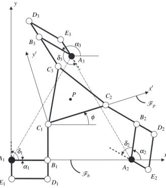
Figure

Documents relatifs
Based on our newly established shareholding classes, we compared performance of four different pair-classes: the state direct control versus the state indirect control, the
We shall see that this phenomenon coincides with an omnipresence of time in society where individuals, confronted with more time, in an ever more disturbing world, find refuge
Abstract—In this paper, we propose a successive convex approximation framework for sparse optimization where the nonsmooth regularization function in the objective function is
Due to the discrete nature of the charge carriers, the current presents some fluctuations (noise) known as shot noise , which we aim to characterize here (not to be confused with
represents an irrational number.. Hence, large partial quotients yield good rational approximations by truncating the continued fraction expansion just before the given
In section 3, we study the regularity of solutions to the Stokes equations by using the lifting method in the case of regular data, and by the transposition method in the case of
In Section 5, we give a specific implementation of a combined MRG of this form and we compare its speed with other combined MRGs proposed in L’Ecuyer (1996) and L’Ecuyer (1999a),
In any 3-dimensional warped product space, the only possible embedded strictly convex surface with constant scalar curvature is the slice sphere provided that the embedded
