Adaptive Wide-Area Closed-Loop Undervoltage
Load Shedding Using Synchronized Measurements
Mevludin Glavic, Senior Member, IEEE
Thierry Van Cutsem, Fellow, IEEE
Abstract—This paper proposes an emergency load shedding
scheme aimed at stopping a developing voltage instability before system disruption. The proposed scheme has a wide-area view of the system, adapts itself to the emergency situation to be handled, and works in closed-loop. It relies on the detection of voltage instability from synchronized measurements recently proposed by the authors. It inherits the assumptions of this detection method (availability of a rich phasor measurement set and communication infrastructure). The method is adaptive in so far as the voltage thresholds used by this undervoltage load shedding scheme are determined from the measurements of the system evolution itself, and the curtailed power is adjusted to the severity of the situation. The features of the proposed scheme are illustrated on a small but realistic system.
Index Terms—Voltage stability, emergency control, load
shed-ding, adaptive control, wide-area measurement system, synchro-nized measurements, sensitivity analysis
I. INTRODUCTION
V
Oltage instability is linked to the inability of the com-bined generation-transmission system to provide the power requested by loads, as a result of equipment outages and limitations of reactive power generation [1], [2]. The voltage instability can evolve in voltage collapse which further can result in partial or widespread system disruption.Different voltage collapse scenarios may evolve depending on the mechanism of load power restoration [2], [3]. In short-term voltage instability, induction motors try to recover their torque in a time frame of typically one second time after the disturbance. In long-term voltage instability, within a few minutes, transformers equipped with Load Tap Changers (LTCs) try to restore their secondary voltages, and hence the corresponding voltage-dependent load powers, while Over-Excitation limiters (OELs) restrict reactive power production from generators.
Control schemes to avoid low voltage situations or stop a de-veloping voltage instability can be categorized into preventive or corrective. Preventive voltage control is designed for a set of credible disturbances and is applied in the pre-disturbance state. These controls are costly since the credible disturbances may never occur in the system. Corrective control, on the other hand, is cost effective in so far as it is triggered when a disturbance actually occurs in the system.
Emergency control is a particular type of corrective control, and can be broadly classified into open loop and closed-M. Glavic (glavic@montefiore.ulg.ac.be) is a visiting professor at the Dept. of Electrical Engineering and Computer Science (Montefiore Institute) of the University of Li`ege, Sart Tilman B37, B-4000 Li`ege, Belgium.
T. Van Cutsem (t.vancutsem@ulg.ac.be) is research director of FNRS (Fund for Scientific Research) and adjunct professor at the same department.
loop [3], [4], [5]. Open-loop emergency control uses actions assessed off-line on the basis of simulations of postulated scenarios and does not re-adjust its actions to follow up the system evolution[1], [4]. On the other hand, closed-loop emergency control assesses the disturbance severity through measurements and adjusts its actions correspondingly, possibly repeating some actions if the previously taken ones are not enough. This allows compensating modelling inaccuracies, and hence makes the control scheme more robust.
Several controls are available to correct abnormal voltages: shunt compensation switching, adjustment of generation volt-age setpoints, modified LTC control, and load shedding [4], [5], [6], [7].
Load shedding is an effective countermeasure in situations when voltage collapse is anticipated [4], [5], [6], [8], [9], [10], [11]. Clearly, it should be used in the last resort, when other available corrective controls have been exhausted, and should be applied automatically, incorporated into a System Integrity Protection Scheme (SIPS) [3], [5], [12].
Most existing undervoltage load shedding schemes rely on local data only, typically one or several bus voltages, possibly complemented by other signals, for instance from neighbouring generators [4]. This makes the SIPS simple and thereby contributes to its reliability. However, the continuous development of communication and measurement technologies (most notably phasor measurement units) have opened new perspectives for designing wide-area monitoring, detection, protection and control systems [12], [13], [14], [15], [16].
In this paper we report on our research efforts to extend the method developed in [15], [16] in order to deploy efficient emergency controls against an impeding voltage instability. More precisely, we concentrate on the design of a closed-loop undervoltage load shedding scheme, leaving aside other possible emergency control actions.
The paper is organized as follows. Some previous develop-ments on voltage instability detection and fast identification of effective controls, are recalled in Section II. An adaptive, closed-loop load shedding scheme is described and illustrated in Section III. Section IV presents simulation results obtained on the Nordic-32 test system, while Section V offers conclu-sions and directions for future research.
II. INSTABILITY DETECTION FROM SYNCHRONIZED MEASUREMENTS
A. Recall of previous developments
In our previous publications [15], [16] we proposed a method for early detection of an impeding voltage instabil-ity from the system states provided by synchronized phasor
measurements. The method fits a set of algebraic equations to the sampled states. These equations are written as:
ϕ(z, s) = 0 (1)
where z is the system state vector and s the vector of active and reactive powers consumed by the loads. Let us emphasize that the method does not require any model of the load response to voltage, only the values of their powers.
Next, sensitivities are used to identify when a combination of load powers passes through a maximum. The sensitivities of the total reactive power generation Qg to individual load reactive powers are considered [2], [15], [16]. Let the reactive powers of the Nl loads be grouped into q = [Q1 . . . QNl]
T. The sought sensitivities are obtained from a general sensitivity formula [2] as: SQgq= −ϕ T q ¡ ϕT z ¢−1 ∇zQg (2)
where ∇zQgdenotes the gradient of Qgwith respect to z, and
ϕq is the Jacobian of ϕ with respect to q. The latter matrix merely includes 0’s and 1’s [15].
At the sought operating point, the above sensitivities change from large positive to large negative values. In theory they should tend to infinity but, in practice, discontinuities and trajectory sampling may prevent them from reaching very high values. What is sought is a sudden change in sign, i.e. we seek to identify a discrete time k such that:
SQgQj(k − 1) > d+ and SQgQj(k) < d− (3)
where d+ > 0 and d− < 0 are thresholds to be adjusted. In the sequel, the point where this condition holds true is referred to as critical point.
Computing SQgqmerely requires solving one linear system
with ϕz as matrix of coefficients and ∇zQg as independent term. The main computational effort lies in the factorization of ϕz, for which efficient sparsity programming packages are
available. Sparse vector techniques could take advantage of the zero components of ∇zQg. Finally, the Jacobian can be limited to the region prone to voltage instability, as shown in [15], [16] where more details about the model can be found.
The important effects of OELs are accounted for through changes in the ϕ function. As explained in [15], an estimate of Eq, the e.m.f. proportional to field current, is used to identify whether a synchronous generator operates under control of its Automatic Voltage Regulator (AVR) or has its field current limited by its OEL. Under AVR control, an equation such as:
Eq− G(Vo− q
v2
x+ vy2) = 0 (4)
is used, while under OEL control, it is replaced by an equation of the type:
Eq− Eqlim= 0 (5)
where G is the open-loop gain and Vo the voltage setpoint of the AVR, vx and vy are the rectangular component of the terminal voltage and Elim
q is proportional to the field current limit.
Furthermore, it is of interest to anticipate the effect of an approaching OEL activation. To this purpose, when Eq >
Elim
q + ², the OEL equation (5) is anticipatively substituted to the AVR equation (4) when evaluating the Jacobian ϕz.
This remains in effect as long as the OEL is acting, which is identified by Elim
q − ² ≤ Eq ≤ Eqlim+ ².
In practice, since Eq may undergo large but short-lasting changes under the effect of electromechanical transients, the inequality Eq> Eqlim+ ² has to hold true for some period of time before the equation is changed.
B. Illustrative example
We give hereafter a short illustrative example, obtained with the test system detailed in Section IV. The case involves a line tripping at t = 12s. The system evolves over some 120 seconds under the effect of LTCs (trying to restore distribution voltages) and OELs acting over several generators. The long-term voltage instability results in a loss of short-term stability in the form of a field current limited generator loosing synchronism. The evolution of the voltage at the bus that experiences the largest drop is shown in Fig. 1.
0 20 40 60 80 100 120 0.7 0.75 0.8 0.85 0.9 0.95 1 Time (s) V (pu) V 1044 A B Pre−alarm (anticipation) Alarm
Fig. 1. Voltage at the transmission bus experiencing the largest drop (uncontrolled system)
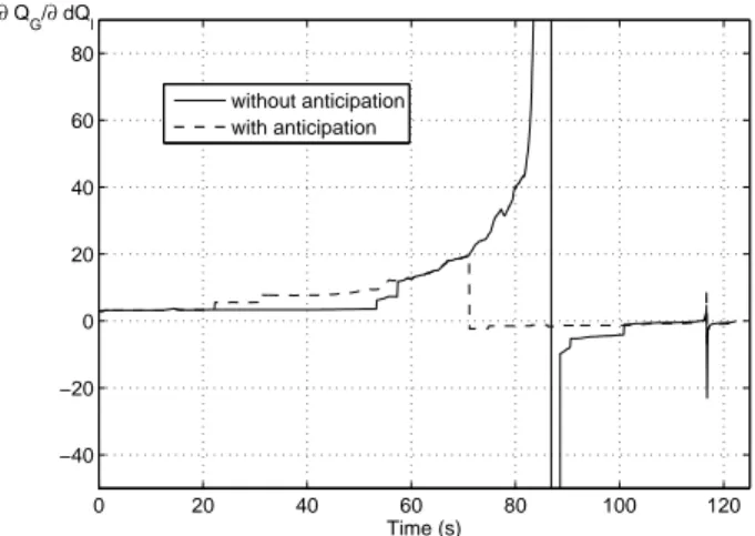
The time evolution of one sensitivity SQgQl, with and
with-out the above mentioned anticipation, is shown in Fig. 2. The change in the sign takes place at t = 71.1 s when anticipation is considered and at t = 86.9 s without anticipation (i.e. 60 and 74.8 seconds after the disturbance, and 51.4 and 35.6 seconds before the collapse). Note that all sensitivities change sign at the same time [15]; only one is shown here for the sake of clarity.
In Fig. 1, the corresponding points are marked A and B, respectively. As can be seen, an early warning of the developing instability is obtained, since at the time of detection the transmission voltages still have acceptable values.
III. ADAPTIVE CLOSED-LOOP UNDERVOLTAGE LOAD SHEDDING
A. Undervoltage load shedding
The type of undervoltage load shedding controller consid-ered in this work obeys the logic shown in Table I, where
0 20 40 60 80 100 120 −40 −20 0 20 40 60 80 Time (s) ∂ QG/∂ dQl without anticipation with anticipation
Fig. 2. Sensitivity at the transmission bus experiencing the largest drop (uncontrolled system)
V is the measured voltage, Vth a threshold value, τ the load shedding delay and ∆P the amount shed at each step.
TABLE I
PSEUDO-CODE OF THE UNDERVOLTAGE LOAD SHEDDING LOGIC
If V drops below Vth at t = t o: repeat at t = to + τ : shed a power ∆P ; set to:= t; until V > Vth endif
The above undervoltage load shedding is simple and works satisfactorily provided appropriate values are chosen for Vth,
τ and ∆P [4], [5], [6], [8], [9]. In some systems, however, it may be delicate to cover a wide range of possible situations with a single value for each parameter, more particularly for Vth. This is where the synchronized measurement based detection outlined in Section II may prove useful. Using this technique, we propose a load shedding scheme that retains the simplicity of the above logic but adapts Vth and ∆P to the situation under concern, as detailed in the remaining of this section.
B. Choosing the voltage threshold Vth
We propose to take for Vth the value of the transmission voltage when crossing the critical point. More precisely, when the sensitivities change sign, a snapshot of each transmission voltage is taken in the region of interest, and the load shedding controller is let to act until all voltages recover above their respective Vth values. The rationale behind this choice is inspired of the simple one-generator one-load system, where it is easily shown that the best strategy is to bring the load voltage at the value where load power is maximum in the post-disturbance configuration [2].
As illustrated in Fig. 2, we have two possible choices, namely with and without anticipation, identified by points A and B, respectively. In fact, point A allows anticipating the
instability but it is at point B that a combination of load powers effectively passes through a maximum. Furthermore, considering the seriousness of a load shedding decision, it is appropriate to have a confirmation that an instability does develop. This confirmation comes from point B following point A. This suggests to “arm” the load shedding controller when crossing point A but activate this emergency control when crossing point B only. In between points A and B, “cheaper” emergency control actions can be deployed, such as LTC blocking, locking, or reversing, shunt capacitors switch-ing, generator setpoints adjustments, etc. This combination of actions is not considered in this paper, which focuses on load shedding.
In practice, it is convenient to compute the sensitivities with anticipation, until reaching point A, from where they can be computed without anticipation, until point B is reached. As already mentioned, this is a matter or choosing between Eqs. (4) and (5) for those generators with the field current exceeding its permanent limit.
C. Choosing the loads to curtail
Various indices can be calculated for ranking buses with respect to their efficiency in boosting voltages through load shedding. In this work, we re-used the sensitivities considered in [17]. They involve the bus voltage Vl that experiences the largest drop at the critical point identified as explained in the previous section. The loads whose change have the greatest impact on Vlare then identified by computing the sensitivities of Vl to the load active powers :
SVlp= −ϕ T p ¡ ϕT z ¢−1 ∇zVl (6) where p = [P1 . . . PNl]
T is the vector of load active powers, and the other symbols have been already defined. Some properties of the above sensitivities have been shown in [17]. They are computed just after crossing the point, before being normalized for ranking purposes.
The loads being ranked by decreasing SVlPi values, the
shedding of a power ∆P will be most effective if applied to the first ranked load, up to the interruptible amount of the latter, then to the second ranked load, and so on until the sum of all interrupted powers reaches the targeted ∆P value [9]. D. Choosing the amount of curtailed power
Information brought by the critical point can be further exploited to estimate the amount of load power to be cut, again with reference to the simple one-generator one-load example. We propose to link the amount of load shedding to the “unrestored power” at the critical point, i.e.
∆Pun = X i∈I
Plipre− Pcrit
li (7)
where Plipreis the pre-disturbance power consumed by the i-th load, Pcrit
li the corresponding value at the critical point, and the sum extends over the set of buses I experiencing voltage drops. This allows the controller to adjust to the severity of the situation. An alternative measure of severity could involve the average voltage drop as in [8], [9], [10].
Let us emphasize that the load shedding controller works in closed-loop by repeating its actions until all voltages are restored (see Table I). Due to this feature, and because ∆Pun may be only a rough estimate of the load to be curtailed, it is appropriate to shed load in successive steps
∆P = α∆Pun 0 < α ≤ 1 (8)
where the α factor should be large enough to avoid delaying the load shedding (and hence either taking the risk of not saving the system, or shedding too much) and small enough to avoid undue shedding and overvoltages. Further considerations on the choice of α and illustrations of its impact are given in the next section.
In the absence of detailed information about the load composition, reactive power was reduced together with active power so as to keep the power factor unchanged, under the pre-disturbance voltage (which is close to the 1 pu setpoint imposed by each distribution LTCs).
E. Choosing the delay τ
The primary purpose of the delay τ is to prevent the controller from reacting to a nearby fault [10]. A larger value may be selected if it is found to yield a smaller total load shedding. However, through studies on real-life systems (e.g. [7], [10]), we observed that in almost all cases shedding small blocks after small delays yielded the smallest total curtailed power. Therefore, in this work, we chose to keep τ as small as possible and set it to 3 seconds in all our simulations.
IV. SIMULATION RESULTS A. Test system and scenarios
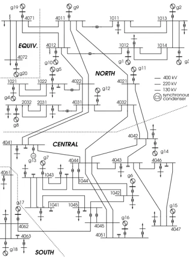
We demonstrate the capabilities of the proposed load shed-ding scheme on the Nordic32 test system, already used in [15], [16]. This is a slightly modified version of the test system detailed in [18].
The one-line diagram of this 52-bus, 20-machine system is shown in Fig. 3.
The model includes for each generator:
• a standard synchronous machine model with 3 or 4 rotor windings (sub-transient time constants taken into account);
• a simple governor (for generators in the North and Equiv areas; the other ones do not participate in frequency control);
• a simple AVR including an OEL.
Each load is represented by an exponential model with ex-ponent 1 (constant current) for the active power and exex-ponent 2 (constant admittance) for the reactive power. In addition, each load is fed through a transformer with automatic LTC. The transformer is assumed ideal for simplicity. There is a delay of 30 seconds on the first tap change and a shorter delay on the subsequent steps.
The model has been implemented in the SIMULINK envi-ronment. A variable step size method is used to simulate its dynamics. Interpolation is used in order to get the system states at regular time intervals (every 100 ms). We do not consider
g20 g16 g17 g18 g2 g9 g1 g3 g10 g5 g4 g12 g8 g13 g14 g7 g6 g15 g11 g19 4011 4012 1011 1012 1014 1013 1022 1021 2031 cs 4046 4043 4044 4032 4031 4022 4021 4071 4072 4041 1042 1045 1041 4063 4061 1043 1044 4047 4051 4045 4062 400 kV 220 kV 130 kV synchronous condenser CS NORTH CENTRAL EQUIV. SOUTH 4042 2032
Fig. 3. Nordic-32 test system
the presence of a (linear) state estimator to process the phasor measurements; we merely use as incoming measurements the projections of each bus voltage phasor on orthogonal axes rotating at the nominal angular speed (these projections are readily available as algebraic variables in the model).
In order to illustrate the adaptiveness of the proposed load shedding, two disturbances are considered (see Fig. 3):
• Case 1: tripping of line 4032-4044
• Case 2: tripping of one of the two parallel circuits between buses 4031 and 4041
both taking place at t = 12 s (for easy visualization of pre-disturbance values). Due to a high power transfer from North to Central areas, the system is not secure with respect to these N-1 contingencies.
B. Results for Case 1
The uncontrolled, unstable system response in terms of voltage at bus 1044, as well as sensitivities with and without anticipation, were given in Figs. 1 and 2, respectively.
The system evolves under the effect of:
• LTCs trying unsuccessfully to restore the distribution voltages (and hence the load powers)
• OELs acting over several machines successively (namely machines: g14 at t = 53.4s, g12 at t = 57.5s, g11 at t = 88.7s, g6 at t = 90.7s and eventually g15 at t =
101.8s), thereby further reducing the power that can be transmitted to loads
• a loss of synchronism of generation g6 leading to the final collapse.
The load ranking outlined in Section III-C is determined just after crossing the critical point B in Fig. 1. The results are given in Table II (see column ”Case 1”). The table also indicates the interruptible power assumed for each load (which is 30 % of the initial load power).
TABLE II
RANKING AND INTERRUPTIBLE POWER OF LOADS Bus ∂V1041/∂p ∂V1041/∂p MW/M var Case 1 Case 2 1041 1.0000 1.0000 180 / 54 1043 0.9135 0.9130 78 / 30 1045 0.8281 0.8303 216 / 69 4051 0.8109 0.8136 240 / 90 1044 0.7874 0.7866 252 / 90
A snapshot of the voltages at the critical point provides the Vth thresholds shown in Table III (see column “Case 1”).
TABLE III
CASE1: VOLTAGE THRESHOLDSVthAT5TRANSMISSION BUSES Bus Case1 Case2
1041 0.9447 0.9710 1043 0.9652 0.9890 1045 0.9484 0.9731 4051 1.0275 1.0419 1044 0.9346 0.9610
The response of the system controlled by load shedding is shown in Fig. 4, in terms of voltage magnitude at bus 1044. The blocks of load shed correspond to two different fractions of ∆Pun, namely α = 1 and α = 0.3. 0 50 100 150 200 250 0.9 0.92 0.94 0.96 0.98 1 Time (s) V (pu) α =1 α =0.3 Load shedding
Fig. 4. Case 1, load shedding with α = 1 and α = 0.3: Voltage at bus 1044 When α = 1.0 the controller acts in a single step on the load at bus 1041 only. On the other hand, Fig. 5 shows how the interrupted power at buses 1041 and 1043 evolves with time, when α = 0.3. These buses are the first two ranked, as shown in Table II. In this case, the controller acts in four
0 50 100 150 200 250 0 20 40 60 80 100 120 140 160 180 Time (s) ∆ P (MW) 1041 1043
Fig. 5. Case 1, load shedding with α = 0.3: interrupted power at two buses
successive steps and disconnects the maximum interruptible part of the load at bus 1041, before resorting to the load at bus 1043. Buses having their voltage below threshold at the succession shedding steps are given in Table IV. The progressive restoration of the voltage profile is easily seen.
TABLE IV
CASE1: BUSES WITHV < VthAT SUCCESSIVE SHEDDING STEPS 1st 2nd 3rd 4th
step step step step 1041 1041 1042 1042 1044 1044 1045 1045 4041 4043 4044 4051
The controller relies on sensitivities until reaching the critical point; beyond that point the voltages are used for simplicity and reliability. It is of interest, however, to see how sensitivities evolve under the effect of load shedding. This is shown in Figs. 6 and Fig. 7, corresponding to α = 1 and α = 0.3, respectively. The sensitivities have been determined without anticipation (as in point B of Fig. 1). It can be seen that restoring all voltages above Vth also restores positive values for the sensitivities. However, it takes more time for them to restore when α = 0.3.
C. Results for Case 2
The evolution of the voltage at bus 1044 in the uncontrolled case is shown in Fig. 8. As in Case 1, the system evolves under the effect of LTCs and OELs. The latter act on g14 at t = 56.2s, g12 at t = 57.4s, g11 at t = 96.3s, g8 at t = 102.1s, g6 at t = 131.7s, and eventually g7 at t = 169.9s). Again, the long-term voltage instability results in a loss of short-term stability in the form of the field current limited generator g6 loosing synchronism. This happens soon after generator g7 also gets limited. The lower number of limited generators and
0 50 100 150 200 250 −100 −80 −60 −40 −20 0 20 40 60 80 100 Time (s) ∂ QG/∂ dQl
Fig. 6. Case 1, load shedding with α = 1.0: sensitivity SQgQlat bus 1044
0 50 100 150 200 250 −100 −80 −60 −40 −20 0 20 40 60 80 100 Time (s) ∂ QG/∂ dQl
Fig. 7. Case 1, load shedding with α = 0.3: sensitivity SQgQlat bus 1044
the longer time before collapse suggest that this case is less severe than Case 1.
0 20 40 60 80 100 120 140 160 0.7 0.75 0.8 0.85 0.9 0.95 1 Time (s) V (pu) A B
Fig. 8. Case 2, uncontrolled: Voltage at bus 1044
0 20 40 60 80 100 120 140 160 −30 −20 −10 0 10 20 30 40 50 60 70 Time (s) ∂ QG/∂ dQl without anticipation with anticipation
Fig. 9. Case 2, uncontrolled: sensitivity SQgQl at bus 1044
0 50 100 150 200 250 0.9 0.92 0.94 0.96 0.98 1 Time (s) V (pu) α =1 α=0.3 Load shedding
Fig. 10. Case 2, load shedding with α = 1 and α = 0.3: voltage at bus 1044
The sensitivities with and without anticipation are given in Fig. 9. Their change in sign gives an early warning of the developing instability. They reach comparatively smaller values (although the change in sign remains pronounced) because the critical point coincides with a generator switching under limit [15].
The ranking of load buses, given in Table II, remains the same, since only slight differences in sensitivity values are observed.
The response of the system stabilized by the load shedding controller is shown in Fig. 10, for α = 1.0 and α = 0.3, respectively.
When α = 1.0, the controller acts in a single step on the load at bus 1041 only, which is the first ranked bus. On the other hand, Fig. 11 shows how the interrupted power at bus 1041 evolves with time, when shedding takes place in successive steps owing to α = 0.3.
A comparison between both cases is given in Table V. Case 1 is more severe than Case 2. In the former, shedding load in a single step leads to shed less power, while in the latter, the
0 50 100 150 200 250 0 20 40 60 80 100 120 Time (s) ∆ P (MW)
Fig. 11. Case 2, load shedding with α = 0.3: interrupted power at the controlled bus
reverse holds true. This raises the issue of choosing a proper value for α. The results suggest that α should be set to a larger value when the unrestored power is larger than the interruptible power at the highest ranked bus(es). This observation is valid for the system of concern here, but additional tests are required to validate it as a general guideline. The tests also show that the unrestored power ∆Pun provides a reasonable reference for the amount of power to shed, and there is no advantage in choosing α > 1.
TABLE V
OVERALL PERFORMANCE OF THE LOAD SHEDDING CONTROLLER Case unrestored total power total power curtailed power shed (in MW) shed (in MW) loads ∆Pun when α = 1 when α = 0.3
1 208 205 254 1041,1043
2 144 144 130 1041
D. Fault-tolerance of the proposed control scheme
Due to its closed-loop nature, the proposed control inher-ently offers some robustness with respect to both operation failures and modelling uncertainties. Among the latter, let us quote the unknown behaviour of loads under low voltage, the load power factor after curtailing part of the load, and some uncertainty on the amount of load actually available for shedding [11].
In order to test the controller robustness we do not randomly perturb control signals (as in [11]) but rather investigate the fault-tolerance of the control scheme facing a failure to activate the expected load shedding.
Two possibilities are envisaged:
• either the controller is informed of the load curtailment failure. This is referred to in Control Systems literature as fault detection and isolation [19];
• or it is not informed, and we rely on the closed-loop structure to compensate for the failure.
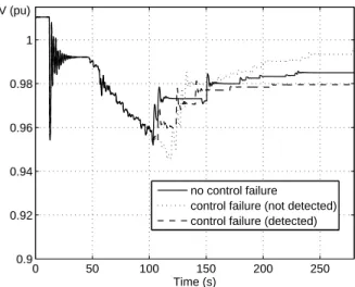
0 50 100 150 200 250 0.9 0.92 0.94 0.96 0.98 1 Time (s) V (pu) no control failure
control failure (not detected) control failure (detected)
Fig. 12. Case 2, shedding with α = 0.3: System responses with and without failure
Figure 12 provides the system responses without failure, with failure and detection, and with undetected failure, re-spectively. They refer to Case 2 and α = 0.3. We assume that the circuit breaker(s) did not operate and failed dropping the load at the first bus selected by the controller (namely 1041). When the load curtailment failure is not known by the controller, the latter keeps on acting virtually on the first ranked load, until the whole interruptible power has been treated by the algorithm of Table I. Then, the controller resorts to the next loads in the list. Of course, in the meantime, the voltages have kept on decreasing. Thus, emergency control is somewhat delayed, although not much thanks to the small value of τ (see Fig. 12). The effective shedding starts at t = 122.2s and takes place in four steps, involving buses 1043 and 1045. The total power curtailed is 288 MW, which is more than in the case without failure (see Table V).
If the curtailment failure is detected and communicated to the controller, the latter immediately reschedules its actions to the next ranked loads. Hence, shedding takes place at buses 1043 and 1045, as in the previous scenario, but with delay of τ = 3 s only with respect to the case without failure (we neglect the communication time from the faulty sub-station to the control center where the load shedding scheme is implemented). The total power curtailed in this case is 222 MW (in three steps), which is less than in the previous scenario, as expected.
Obviously, detecting the failure allows better performances in terms of load shedding. However, this detection may not be easy or affordable in some systems, as it requires additional, fast communication. This also depends on how load shedding is implemented down to the end-consumer [11]. Hence, the fact that the scheme can also work without this detection is an interesting feature.
V. CONCLUSION
In this paper we have presented some results of research efforts to exploit future possibilities offered by synchronized
measurements, applied to voltage instability detection and con-trol. The application shown here is in the direct continuation of the work reported in [15], [16].
The proposed load shedding scheme is adaptive in terms of voltage thresholds and amount of load shedding. The former are the voltages collected at the critical point (where sensitiv-ities change sign passing through large values). The latter is linked to the so-called unrestored load power, determined at the same point.
Further efforts are needed to fully demonstrate the potentials of designing adaptive closed-loop emergency controls along the ideas presented in this paper. Nevertheless, the presented results already show good promises.
Among the points of interest for future investigations, let us quote the inclusion of generator voltages in the controller logic, in order to deal with generators operating above the field current limit (whose OEL is going to act after an overload period). In this case, load shedding would be also aimed at keeping generators under AVR control. Another topic of interest is the combination of various emergency controls using the capability of sensitivities to provide a pre-alarm (when computing them with the OEL limits anticipated), as outlined in the paper.
ACKNOWLEDGMENTS
M. Glavic acknowledges FNRS (Belgian National Fund for Scientific Research) for supporting his research stays at the University of Li`ege through the visiting professor grants. T. Van Cutsem is a research director of FNRS.
REFERENCES
[1] C. W. Taylor, Power System Voltage Stability, EPRI Power System Engineering Series, McGraw Hill, 1994
[2] T. Van Cutsem, C. Vournas, Voltage Stability of Electric Power Systems, Boston, Springer (previously Kluwer Academic Publishers), 1998 [3] D. H. Karlsson (Convener), “System Protection Schemes in Power
Networks,” CIGRE Task Force 38.02.19
[4] T. Van Cutsem, C. D. Vournas, “Emergency Voltage Stability Controls: An Overview,” in Proc. IEEE PES General Meeting, Tampa, Jun. 2007 [5] V. C. Nikolaidis, C. D. Vournas, “Design Startegies for Load Shedding
Schemes Against Voltage Collapse in the Hellenic System,” IEEE Trans. Power Syst., Vol. 23, No. 2, pp. 582-591, May 2008
[6] C. W. Taylor, “Concepts of Undervoltage Load Shedding for Voltage Stability,” IEEE Trans. Power Del., Vol. 7, No. 2, pp. 480-488, Apr. 1992
[7] F. Capitanescu, B. Otomega, H. Lefebvre, V. Sermanson, T. Van Cutsem, “Decentralized tap changer blocking and load shedding against voltage instability: Prospective tests on the RTE system,” Int. Journal Elec. Power and Energy Syst., Vol. 31, pp. 570-576, 2009
[8] C. Moors, D. Lefebvre, T. Van Cutsem, “Load Shedding Controllers Against Voltage Instability: a Comparison of Designs,” in Proc. IEEE Power Tech Conference, Porto, Portugal, 2001
[9] C. Moors, “On the Design of Load Shedding Schemes Against Voltage Instability in Electric Power System,” PhD Thesis, University of Li`ege, Belgium, 2003
[10] B. Otomega, T. Van Cutsem, “Undervoltage Load Shedding Using Distributed Controllers,” IEEE Trans. Power Syst., Vol. 22, No. 4, pp. 1898-1907, Nov. 2007
[11] I. Hiskens, B. Gong, “Volatge Stability Enhancement via Model Predic-tive Control of Load,” Int. Automation and Soft Comp., Vol. 12, No. 1, pp. 117-124, 2006
[12] B. Milosevic, M. Begovic, “Voltage Stability Protection and Control using a Wide-Area Network of Phasor Measurements,” IEEE Trans. Power Syst., Vol. 18, No. 1, pp. 121-127, Feb. 2003
[13] A. G. Phadke, J. S. Thorp, Synchronized Phasor Measurements and Their Applications, Springer, 2008
[14] D. Novosel, V. Madani, B. Bhragava, K. Vu, J. Cole, “Dawn of the Grid Synhronization: Benefits, Practical Applications, and Deployment Strategies for Wide Area Monitoring, Protection, and Control,” IEEE Power and Energy Magazine, pp. 49-60, Jan./Feb. 2008
[15] M. Glavic, T. Van Cutsem, “Wide-Area Detection of Voltage Instability From Synchronized Phasor Measurements. Part I: Principle,” IEEE Trans. Power Syst., Vol. 24, No. 3, pp. 1408-1416, Aug. 2009
[16] M. Glavic, T. Van Cutsem, “Wide-Area Detection of Voltage Instability From Synchronized Phasor Measurements. Part II: Simulation Results,” IEEE Trans. Power Syst., Vol. 24, No. 3, pp. 1417-1425, Aug. 2009 [17] F. Capitanescu, T. Van Cutsem, “Unified sensitivity analysis of unstable
or low voltages caused by load increases or contingencies,” IEEE Trans. Power Syst., Vol. 20, No. 1, pp. 321-329, Feb. 2005
[18] M. Stubbe (Convener), Long-Term Dynamics - Phase II, CIGRE TF 38.02.08, CIGRE Technical brochure, Jan. 1995
[19] H. Noura, D. Theilliol, J-C. Ponsart, A. Chamseddine, Fault-tolerant Control Systems, Springer, 2009