Study of Polyethylene Crystallization

Étude de la Cristallisation du Polyéthylène

par

Azar Shamloo

Thèse présentée au Département de chimie en vue

de l’obtention du grade de Philosophia doctor (Ph.D.)

FACULTÉ DES SCIENCES, UNIVERSITÉ DE SHERBROOKE

i

Study of Polyethylene Crystallization

By

Azar Shamloo

Thesis presented in the chemistry department for obtaining the degree of

Doctor of Science (Ph.D.)

FACULTY OF SCIENCES

UNIVERSITÉ DE SHERBROOKE

i

Le 13 Juin 2018

Le jury a accepté la Thèse de Madame Azar Shamloo dans sa version finale.

Jury Members

Professor Armand Soldera

Research Director

Department of Chemistry

Professor Denis Rodrigue

Research Codirector

Department of Chemical Engineering

Université Laval

Professor Veena Choudhary

External evaluator

Centre For Polymer Science and Engineering

Indian Institute of Technology, Delhi

Professor Patrick Ayotte

Internal evaluator

Department of Chemistry

Professor Mathieu Robert

Internal evaluator

Department of Civil Engineering

Professor Jean-Philippe Bellenger

Committee President

ii

RÉSUMÉ

Dans l'industrie, les produits finis en plastique sont fabriqués par diverses techniques de traitement telles que le moulage par compression, le moulage par injection, le moulage par soufflage, l'extrusion, etc. Ces opérations impliquent l'exposition de résines polymères à de nombreux conditions telles que la température, pression, contrainte, etc. Certaines conditions sont connues pour affecter la nature de la structure cristalline des polymères semi-cristallins qui est contrôlée par des mécanismes de cristallisation. Pour un matériau tel que le polyéthylène (PE), la structure de la chaîne polymère influence la morphologie et la cristallinité. Les nanocristaux de PE ont attiré une attention considérable en raison des applications potentielles dans la technologie et de leurs propriétés fascinantes qui sont différent clairement des leurs matériaux en vrac correspondants. Il existe plusieurs méthodes pour déterminer la cristallinité du polymère, mais la plupart d'entre elles sont destructrices et fournissent des informations ponctuelles. Elles nécessitent également souvent un temps de manipulation important, tandis que les expériences sur des objets à l'échelle nanométrique sont souvent restées avec une grande incertitude en raison de la difficulté de produire et de manipuler ces objets à des échelles de longueur inférieures à 10 nm. Pour ces raisons, les méthodes de calcul sont considérées comme des outils parfaits pour mieux comprendre ces observations expérimentales.

La finalité de cette étude vise à révéler l'effet des conditions environnementales sur la température de fusion des nanocristaux de chaînes alcanes en utilisant tant des simulations de dynamique moléculaire afin de représenter au mieux des composés réels ainsi que des techniques expérimentales pour étudier les conditions de traitement sur leur tension interfaciale. Il a été montré que la loi de Gibbs-Thomson peut être reproduite, car cette loi dévoile une relation linéaire entre la température de fusion et l'inverse de l'épaisseur du cristal. Pour révéler efficacement l'impact des conditions environnementales sur le comportement de fusion PE, un nanocristal composé de chaînes d'alcane est incorporé dans une phase amorphe. Finalement, l'étude du comportement de fusion et de cristallisation des polymères sous haute pression a un intérêt fondamental pour la compréhension de la structure du polymère. Suite à notre travail sur le

iii

nanocristal chaînes d'alcane, nous avons calculé la valeur de la tension interfaciale à différentes pressions pour explorer l'effet de ce paramètre sur la température de fusion et la tension interfaciale de ce matériau. Plus précisément:

a) Nous avons démontré que la température de fusion augmente et la tension interfaciale diminue, en comparant les résultats obtenus avec des chaînes d'alcanes nanocristal incorporées dans une phase amorphe avec un nanocristal isolé. Cela peut se révéler grâce au comportement du déplacement quadratique moyenne d'une particule près de la surface du cristal dans les deux systèmes (chaînes d'alcanes nanocristal incorporées dans une phase amorphe avec un nanocristal isolé). Les interactions entre les monomères non liés dans nanocristal chaînes d'alcane et alcanes dans la phase amorphe diminuent la mobilité des chaînes dans le cristal conduisant à une température de fusion plus élevée et une tension interfaciale plus faible.

b) Il a été montré que l'augmentation de la pression entraîne une diminution de la tension interfaciale, ce qui peut s'expliquer par une diminution de l'énergie libre de Gibbs. De plus, en comparant les expériences et les données de simulation, nous obtenons une correspondance précise qu'en augmentant la pression, le point de fusion des échantillons augmentera aussi.

Dans la partie expérimentale, l'effet de la température du moule, de la pression du moule, du taux de refroidissement et du profil de température sur les propriétés thermiques et mécaniques des échantillons sont étudiés. Les résultats confirment que pour des échantillons symétriques (température de moulage uniforme), une température de fusion, les modules de flexion et de traction plus élevées découlent d'une augmentation de la pression et la température de moulage, tout en diminuant la vitesse de refroidissement.

D'autre part, pour les échantillons asymétriques où le gradient de température est appliqué lors du moulage, le module de traction et de flexion ne dépend pas seulement de la différence de température, mais aussi de la température moyenne entre les plaques supérieure et inférieure de la presse à mouler par compression. On observe que les modules de traction et flexion les plus élevés

iv

sont obtenus pour la température la plus basse sur les deux plaques. Ce comportement peut être clairement révélé en utilisant le rapport de module de flexion qui représente la valeur mesurée lorsque la charge est appliquée sur les côtés supérieure et inférieure (Eb / Eu). Enfin, il a été montré que l'augmentation de la pression de moulage entraîne une tension interfaciale la plus basse qui peut s'expliquer par une diminution de l'énergie libre de Gibbs pendant la cristallisation. Ce résultat a également confirmé les données de simulation.

v

SUMMARY

In industry, end user plastics products are made by diverse polymer processing techniques such as compression molding, injection molding, blow molding, extrusion, etc. These processing operations involve exposing polymer resins to elevated temperatures, pressures, stresses, strains, etc. All these conditions are known to affect the nature of the crystalline structure of semi-crystalline polymers and is referred to as morphology which is controlled by crystallization mechanisms. For a material such as polyethylene (PE), the polymer chain structure influences on morphology and crystallinity. PE nanocrystals have attracted considerable attention due to potential applications in technology and their fascinating properties which clearly differ from those of their corresponding bulk materials. Nowadays, different methods are used to determine polymer crystallinity, but most of them are destructive and provide single point information. They also often require significant handling time, while experiments on nanoscale objects are often plague with high uncertainty because of the difficulty of producing and manipulating these objects at length scales below 10 nm. For these reasons, computational methods are seen as perfect tools to get more insight into these experimental observations.

This work is thus aimed at revealing the effect of environmental conditions on the melting temperature of alkane chains nanocrystals using molecular dynamics simulations to approach real compounds. It was shown that the Gibbs-Thomson law can be reproduced, as this law unveils a linear relationship between the melting temperature and the inverse of the crystal thickness. To efficiently reveal the impact of environmental conditions on the melting behaviour of PE, a nanocrystal composed of alkane chains is embedded in an amorphous phase. Ultimately, the investigation of the melting and crystallization behaviour of polymers under high pressure has basic interest for the understanding of the polymer structure. Following our work on polyethylene nanocrystal, we calculated the value of interfacial tension at different pressures to explore the effect of this parameter on melting temperature and interfacial tension of this material. More specifically:

vi

a) We demonstrated that melting temperature increases and interfacial tension decreases, comparing the results from single alkane chains nanocrystal embedded in an amorphous phase with isolated crystal. This can be explained by MSD (Molecular Dynamic Simulation) behaviour of one particle near the crystal surface in both systems (single alkane chains nanocrystal embedded in an amorphous phase with isolated crystal). Interactions between unbonded monomers in crystal and alkane chains in the amorphous phase decrease the chains mobility in the crystal leading to higher melting temperature and lower interfacial tension.

b) It was shown that increase of pressure results in decrease of interfacial tension, which can be explained by depression in Gibbs free energy. Furthermore, comparing experiments and simulation data give us an accurate match that by increasing pressure, melting point of samples will increase too.

In experimental part, the effect of mold temperature, mold pressure, cooling rate and temperature profile on the thermal and mechanical properties of the samples are investigated. Results confirm that for symmetric samples (uniform molding temperature), higher melting temperature, flexural and tensile modulus stem from an increase in the molding pressure and molding temperature, while decreasing the cooling rate.

On the other hand, for asymmetric samples where temperature gradient is applied while molding, the tensile and flexural modulus not only depend on the temperature difference, but also on the average temperature between the upper (Tu) and bottom (Tb) plates of the compression molding press. It is observed that the highest tensile and flexural moduli are obtained for the lowest temperature on both plates. This behavior can be clearly revealed using the flexural modulus ratio which represents the value measured when the load is applied on the bottom or the upper sides (Eb/Eu). Finally, it was shown that increasing the molding pressure results in lower interfacial tension which can be explained by a depression of the Gibbs free energy during crystallization. This result confirmed simulation data as well.

vii

ACKNOWLEDGMENTS

This thesis has been a great experience that would not have been possible without the support of many great individuals. My thanks and appreciation to all of them for all their effort, motivation and support during this study.

First and foremost, I would like to express my sincere gratitude to my advisor Prof. Armand Soldera for the continuous support of my Ph.D. study and related research, for his patience, motivation, and immense knowledge. His guidance helped me in all the time of research and writing of this thesis. I am glad to have had this opportunity to work in his lab, the Laboratory of Physical Chemistry of Matter (LPCM).

My sincere thanks also go to my codirector Prof. Denis Rodrigue who provided me an opportunity to join their team at Université Laval, and who gave access to the laboratory and research facilities. Without his precious support it would not be possible to conduct this research. In addition to his scientific support, his guidance and advice has helped me during the entire duration of research and writing for this thesis.

A very special gratitude goes out to Prof. Said Elkoun who allowed me to work and use research facilities in his laboratory in engineering department. His advice and support while writing the article was very precious for me.

Besides my advisors, I would like to thank the rest of my thesis committee: Prof. Veena Choudhary (external evaluator), Prof. Patrick Ayotte (head of the department of chemistry), Prof. Mathieu Robert and Prof. Jean-Philippe Bellenger (the chairman of the committee), agreeing to be my referees. I would also like to thank the rest of the faculty and staff in the Department of Chemistry at the Université de Sherbrooke. In particular, I would like to thank Dr. Jean-Marc Chapuzet, academic coordinator at the Department of Chemistry for his good humor and help.

viii

I would especially like to thank my amazing family for the love, support, and constant encouragement I have gotten over the years. Especially my mother who have supported me along the way. I am grateful to my husband, Vahid, who have provided me through emotional support in my life.

I want to express my deep appreciation for the help and support of my colleagues: Dr. François Porzio, Dr. Nasim Anousheh, François Godey, Vincent St-Onge, Clément Wespiser, Alexandre Fleury and Étienne Cuierrier.

This work was supported by the Centre Québécois sur les Matériaux Fonctionnels (CQMF) and the Fonds Québécois de la Recherche sur la Nature et les Technologies (FQRNT), and Université de Sherbrooke.

This dissertation is dedicated to my father who always inspired me. He dedicated his life to help the others. He is my hero as long as I live.

ix

ABBREVIATIONS

ABS Acrylonitrile Butadiene Styrene

AMBER Assisted Model Building with Energy Refinement B-PE Branched Polyethylene

CHARMM Chemistry at HARvard Macromolecular Mechanics CG Coarse-Grained

CNC Computer Numerical Control CW Constant Wavelength

DSC Differential Scanning calorimetry EVA Ethylene-Vinyl Acetate Copolymer G-T Gibbs -Thomson Equation

HDPE High Density Polyethylene IBC Isolated Boundary Condition

LBFGS Limited-memory Broyden-Fletcher-Goldfarb-Shanno quasi-Newtonian minimizer

LLDPE Linear Low-Density Polyethylene LDPE Low Density Polyethylene

MC Monte Carlo Simulation

MD Molecular Dynamics Simulation MSD Mean Square Deviation

x

OPLS Optimized Potentials for Liquid Simulations PBC Periodic Boundary Condition

PC Polycarbonate PE Polyethylene

POM Polarized Optical Microscopy PVA Poly (Vinyl Alcohol)

QSPR Quantitative Structure Property Relationships RIS Rotational Isomeric States

SAXS Small Angle X-ray Scattering Tm Melting Temperature

Tg Glass Transition Temperature UA United-Atom

VLDPE Very Low-Density Polyethylene XRD X-ray Diffraction

xi Table of Contents RÉSUMÉ ... ii SUMMARY ... v ACKNOWLEDGMENTS ... vii ABBREVIATIONS ... ix Table of Contents ... xi LIST OF FIGURES ... xv

LIST OF TABLES ... xvii

CHAPTER I. Literature Review and Objectives of Project ... 7

1.1. Introduction to Polyethylene ... 7

1.1.1 High Density Polyethylene ... 7

1.1.2. Low Density Polyethylene ... 7

1.1.3. Linear Low-Density Polyethylene ... 7

1.1.4. Very Low-Density Polyethylene ... 7

1.1.5. Spherulite Structure ... 8

1.1.6. Crystalline Structure ... 8

1.1.7. Intrinsic Properties ... 9

1.1.8. High Density Polyethylene Synthesis... 10

1.1.9. Low Density Polyethylene Synthesis ... 10

1.2. Models for Semi-Crystalline Polymers ... 10

1.2.1. Fringed-Micelle Model ... 10

1.2.2. Chain-Folding Model ... 11

1.3. Flory’s Crystallization Theory for Homopolymers ... 12

1.4. Lamellar Thickness in Polymers ... 15

1.5. Gibbs-Thomson Equation ... 15

1.6. Thermodynamics of Fusion ... 18

1.7. Objectives of Project ... 21

CHAPTER II. Review of Polymer Simulation Methods and Molecular Dynamics... 23

xii

2.2. Simulation of Polymers ... 23

2.2.1. Polymers Properties ... 24

2.3. The Objective of Molecular Dynamics ... 26

2.4. Time Dependence ... 28

2.5. Non-bonded Interaction... 28

2.6. Bonding Potentials ... 29

2.7. Validation of Force Fields ... 31

2.8. The MD Algorithm... 32

2.9. The Velocity Verlet Algorithm ... 32

2.10. Molecular Dynamics Methods ... 33

2.11. Boundary Conditions ... 35

2.11.1. Periodic Boundary Condition ... 35

2.11.2. Isolated Boundary Condition (IBC) ... 37

2.12. Ewald Summation ... 37

2.13. Neighbor Lists ... 37

2.14. Molecular Dynamics in Different Ensembles ... 38

2.15. Energy Minimization... 40

2.15.1. Steepest Descent ... 41

2.15.2. Conjugate Gradient ... 42

2.15.3. L-BFGS ... 42

2.16. Cell Construction... 42

2.17. Making the Configuration (PE Nanocrystal embedded in Amorphous Phase) ... 44

2.18. Hydrostatic Uniform Compression ... 47

2.19. Melting Simulation ... 47

2.20. Errors and Uncertainty in MD Simulation ... 47

CHAPTER III. Review of Molding Methods and Effect of Processing Conditions on the Thermal and Mechanical Properties of Polymers ... 50

3.1. Introduction ... 50

3.2. Types of Plastics... 50

xiii

3.3.1 Injection Molding ... 51

3.3.2 Compression Molding ... 52

3.4. Mechanical Properties of Polymers... 53

3.4.1. Elasticity ... 53

3.4.2. Strength ... 53

3.4.3. Elongation to Break (Ultimate Elongation) ... 54

3.4.4. Young’s Modulus (Modulus of Elasticity or Tensile Modulus) ... 54

3.4.5. Toughness ... 54

3.5. Melting Point and Glass Transition Temperature of Polymers ... 56

3.6. Polymer Crystallinity: Crystalline and Amorphous Polymers ... 57

3.7. Surface Tension of Polymers ... 58

3.8. Experimental Work ... 58

3.9. The Effect of Hydrostatic Pressure on Mechanical Properties of Polymers ... 61

3.10. Melting of Polymers under high Pressure ... 62

3.11. Cooling Rate via Crystallinity and Melting Temperature ... 63

3.12. Molding Temperature via Mechanical Properties, Crystallinity and Melting Point ... 63

CHAPTER IV. Influence of Compression Molding Conditions on the Thermal and Mechanical Properties of LDPE (Low Density Polyethylene) ... 65

4.1. Introduction ... 65

4.2. Influence of Mold Temperature, Pressure and Cooling rate on the Thermal Properties of Symmetric and Asymmetric LDPE Samples ... 65

4.3. Mechanical Properties of Symmetric and Asymmetric LDPE Samples ... 71

4.4. Conclusion ... 76

Chapter V: Melting of Alkane Nanocrystals: Towards a Representation of Polyethylene ... 78

5.1. Introduction ... 78

5.2. Molecular Dynamic Simulation of Alkane Chains Nanocrystal embedded in an Amorphous phase: Melting Temperature and Surface Tension via the Gibbs-Thomson Equation ... 79

5.3. Pressure Effect on the Melting Behavior of Alkane Chains Nanocrystals: Molecular Dynamic Simulation ... 87

xiv

Conclusion ... 91 APPENDIX I ... 94 Bibliography ... 98

xv

LIST OF FIGURES

Figure 1. The general structure of high density, low density and linear low density polyethylene 8 Figure 2. Schematic representation of: a) spherulite structure [53] and b) crystalline structure [52] ... 9 Figure 3. Schematic of: a) fringed-micelle model for semi-crystalline polymers, b) chain-folded lamellar structure with adjacent re-entry and c) switchboard random [59] ... 12 Figure 4. Diagram of a crystalline polymer lamella. ... 16 Figure 5. Variation of Tm as a function of length expressed as1/x̄ ... 17 Figure 6. Variation of temperatures with respect to the inverse of crystal thickness for the

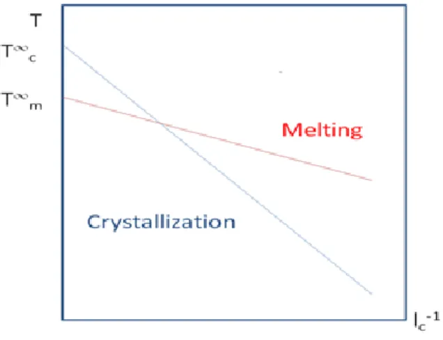
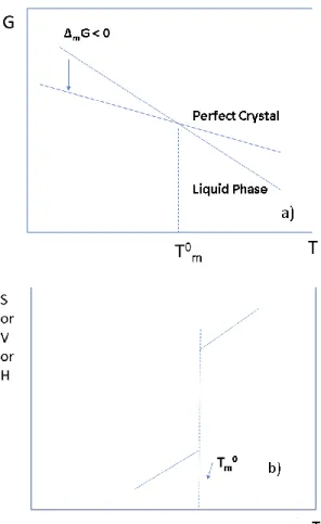
crystallization (blue) and melting line (red)... 19 Figure 7. General behavior of thermodynamic variables at the equilibrium melting temperature Tm0_{: (a) Gibbs free energy and (b) entropy, enthalpy and volume ... 20} Figure 8. Simulations act as a bridge between different scales: (a) microscopic and (b)

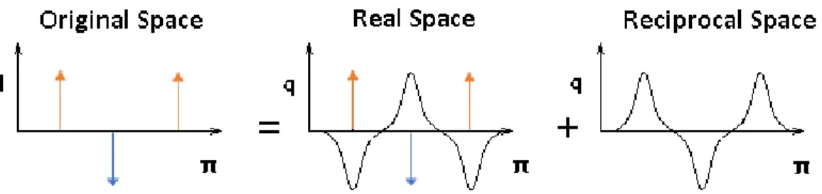
macroscopic ... 27 Figure 9. Geometry of a simple chain molecule illustrating the definition of interatomic distance r23, bend angle 234, and torsion angle 1234 [83] ... 30 Figure 10. Schematic representation of a periodic boundary [115] ... 36 Figure 11. Five types of periodic boundary boxes: (a) the triclinic box, (b) the hexagonal prism, (c) the rhombic dodecahedron, (d) the elongated rhombic dodecahedron, and (e) the truncated octahedron [115]. ... 36 Figure 12. The method of Ewald summation for periodic potentials including the real, reciprocal and original spaces ... 38 Figure 13. The potential cutoff range (solid circle) and the list range (dashed circle), are

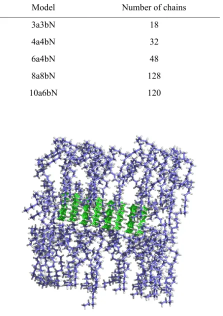
indicated (a). The list must be reconstructed before the particles originally outside the list range (red) have penetrated the potential cutoff sphere [89] ... 39 Figure 14. Random-walk of a polymer chain. ... 43 Figure 15. Simple example of a scanning procedure. A filled circle presents the last segment added, empty circles are occupied space, and a square represents the free space. ... 44 Figure 16. Representation of a polyethylene nanocrystal embedded in alkane chains (amorphous phase) ... 46 Figure 17. Determination of the melting temperature by MD for the crystal 4a4b4cembedded in an amorphous phase (duration 500 ps). (a) Potential energies, (b) heat capacity at constant

volume with respect to temperature, and (c) trans-rotameric state ... 49 Figure 18. Schematic representation of: a) thermoplastic structure and b) thermoset structure ... 50 Figure 19. Representation of the elongation at break and ductility ... 54 The toughness represents the energy absorbed by the material before it breaks. A typical stress-strain curve is shown Figure 21. ... 54

xvi

Figure 20. Typical stress-strain curve to calculate the mechanical properties ... 55 Figure 21. Stress-strain behavior of different materials: a) brittle polymer (glassy polymer/low temperature thermoset), b) ductile polymer (semi-crystalline polymer/plastic/elevated

temperature thermoplastic), and c) highly elastic (elastomer) ... 55 Figure 22. Melting point and glass transition of polymers ... 57 Figure 23. A p-value related to the probability of an observed result ... 66 Figure 24. Melting point, heat of fusion and degree of crystallinity of the samples produced at 3 MPa and 135, 150 and 165 o_{C ... 67} Figure 25. Melting point heat of fusion and degree of crystallinity for the samples produced at 150 °C and 11, 17, 22 and 28 MPa ... 68 Figure 26. Diffractograms of LDPE for different molding conditions: (a) 3 MPa and different cooling rates, (b) 3 MPa and 135, 150 and 165 o_{C, and (c) 150 °C and 11, 17, 22 and 28 MPa .. 71} Figure 27. Surface tension of the samples produced under different molding pressure, as

measured in water and n-hexane. ... 76 Figure 28. Simulated Tm from Eqn. (5.2) for l: 1.01, 1.26, 1.52, 2.03 and 3.04 nm (c = 2.5534 Å, explained in 2.17.) to 1/x. ... 80 Figure 29. Gibbs-Thomson representation of the experimental (circle) and simulated (square) Tm as a function of 1/l for isolated alkane chains nanocrystal and compared with the simulated (triangle) Tm for alkane chains nanocrystal in an amorphous phase. ... 81 Figure 30. Mean square deviation of one particle on surface of alkane chains crystal at T=440 K T>Tm by 4a4b5c, isolated alkane chains crystal (square), alkane chains crystal within amorphous phase (circle) and one particle in amorphous phase(triangle). ... 83 Figure 31. Modified Gibbs-Thomson equation representation reporting experimental (circle) and simulated (square) Tm/To_{m for isolated alkane chains nanocrystal and experimental (inverted} triangle) simulated (triangle) Tm for alkane chains nanocrystal in amorphous phase versus 1/l .. 84 Figure 32. Gibbs-Thomson representation of the simulated Tm versus 1/l at 0 (square), 1000 (circle), 1500 (triangle), and 2000 (inverted triangle) atm. ... 88 Figure 33. Effect of pressure on melting temperature of Polyethylene crystal: Comparison

between experimental (circle) [7] and simulation (square) data by 4a4b3c alkane chains crystal within amorphous phase ... 89

xvii

LIST OF TABLES

Table 1. Main polyethylene properties ... 9

Table 2. Configuration and nanocrystals chain numbers ... 46

Table 3. Sample codes and molding conditions to produce the samples ... 58

Table 4. Sample code, molding conditions, melting point, heat of fusion and degree of crystallinity of the samples produced at 3 MPa and different temperatures ... 65

Table 5. Sample code, molding conditions, melting point, heat of fusion and degree of crystallinity for the samples produced at 150 °C and different pressures... 67

Table 6. Molding conditions, melting point, heat of fusion and degree of crystallinity for the samples produced at 3 MPa and different cooling rates ... 68

Table 7. Molding conditions, melting point, heat of fusion and degree of crystallinity for the samples produced at 3 MPa and different temperature profiles ... 69

Table 8. Molding conditions, tensile strength, elongation at break, flexural and Young’s moduli for the samples produced at 3 MPa and different temperatures ... 69

Table 9. Molding conditions, tensile strength, elongation at break, flexural and Young’s moduli for the samples produced at 150 °C and different pressures ... 71

Table 10. Molding conditions, tensile strength, elongation at break, flexural and Young’s moduli for the samples produced at 3 MPa and different cooling rates. ... 72

Table 11. Molding conditions, tensile strength, elongation at break, flexural and Young’s moduli for the samples produced at 3 MPa and different temperature profiles ... 74

Table 12. Slope (ɑ) and the ordinate at the origin (β(l) of Eqn.(2) for different l values. ... 79

Table 13. Crystal dimensions, enthalpy, entropy, surface tension, difference of energy, melting temperature and volume of alkane chains nanocrystal. ... 85

Table 14. Parameters for non-bonding energetic term... 93

Table 15. Partial charge for nonbonding energetic term... 94

Table 16. Parameters for bonding energetic term ... 94

Table 17. Parameters for valence energetic term ... 94

Table 18. Parameters for dihedral angle energetic term ... 95

Table 19. Parameters for cross terms (bond-bond, bond-angle) ... 95

Table 20. Parameters for cross terms (angle-angle)... 95

Table 21. Parameters for cross terms (End_bond-torsion, middle_bond-torsion); (kcalmol-1_Å-1_{) 96} Table 22. Parameters for cross terms (angle-angle, Angle-angle-torsion); (kcalmol-1_deg-1_{) ... 96}

1

INTRODUCTION

A) Investigation of Melting Point and Interfacial Tension using Gibbs-Thomson Equation in Polyethylene Nanocrystal System (Simulation Study)

The concurrent presence of crystal and amorphous components among bulk semi-crystalline polymers definitively explain the difference between the melting and crystallization temperatures, which is not witnessed in low molar mass systems. The crystallization phenomenon recently became a source of debate, revealing that both melting, and crystallization are not clearly understood. The slope difference in the Gibbs-Thomson (GT) equation observed between both phenomena increases this debate. Thanks to molecular simulations providing a description of interactions between atoms, interesting information can be obtained for a better description of these phenomena. Recently, our group showed that the melting of nanocrystals constituted of alkane chains obeys the GT equation as very good agreement was obtained with experimental data [1]. Here, we propose to approach the real polymer, and thus to unveil the GT equation, by embedding the nanocrystals of alkane chains in an amorphous phase using MD simulation. It is known that polymer chain connectivity and interface have an important effect on the crystals structure leading to different properties. The presence of amorphous regions and their connectivity through chains and adjacent lamellae influence the high degree of plastic deformation in polymers. When the chains are very short, insufficient “tie chains” between the lamellae produces brittleness in the materials [2]. In addition, it was observed that the properties of nanomaterials and their corresponding bulk materials are different [3, 4]. The predominance of interfacial phenomena leads to variation of the macroscale law to the nanoscale field [5]. The physico-chemical processes occurring within length scales of surfaces and interfaces of a few Angstroms are responsible for wetting, adhesion, friction, crystal growth and many other materials phenomena. The bulk processes play very important role in material function like for the rheological properties and adhesion of a pressure-sensitive adhesive. However, its complete behavior is often limited by the processes occurring at the interfaces. This is why material scientists try to explain interfacial phenomena on some common grounds based on two fundamental interface properties: energetics of interactions and dynamics [6].

2

One of the most significant physico-chemical parameters in several polymer engineering processes, such as fiber, film and foam processing, is interfacial tension (g) [7]. In general, interfacial tension decreases with increasing pressure which can be explained by the decreasing Gibbs free energy during crystallization at high pressure-induced crystallization in comparison with ambient conditions [7]. The self-consistent field theory (SCFT) [8] and experimental data both confirm this behavior interfacial tension can be obtained from the change of Gibbs free energy (G) with respect to the surface area (A) at constant temperature (T) and pressure (P) as:

g = (¶G_¶A) 𝑇,𝑃

SCFT is an equilibrium statistical mechanical approach to determine morphology in polymer systems. The free energy function is minimized to find the lowest energy morphology by this method. The procedure for deriving such function is explained in a number of review papers [9-12]. Because of limited amount of information available for nanocrystal polymers such as polyethylene produced at high pressure and temperature, more in depth studies on the effect of processing conditions and polymer chain structure are definitely important to improve our knowledge about the parameters controlling the ultimate materials properties [13].

The other factors controlling the nanocrystal properties are nanoparticles size and dimension [14,15]. It was observed that melting temperature and enthalpy both depend on the polymer nanocrystal size [16,17]. The size effect can be seen in the GT equation, and the interfacial effects need to be considered. The melting temperature of n-alkanes in bulk was reported in NPT (constant pressure and temperature) ensemble [18]. Furthermore, the melting transition of polymer crystals

like isotactic polypropylene and polyethylene were investigatedusing atomistic simulation [19]. The melting transition points of functionalized polyolefins was studied as approximated by nanoparticles and their behavior was demonstrated [20]. The effect of nanoparticle size on the melting point of polymers has been shown. This size effect will be discussed in our system as well. Nowadays, different methods are used to determine polymer crystallinity and melting, but most of them are destructive. They often require significant experimental (handling, preparation and

measurement) time. Experiments on nanoscale objects are often limited by uncertainty because of

the difficulty of producing and manipulating these objects at length scales below 10 nm. Moreover, (1)

3

it has been difficult to synthesize polymer crystals of such small size especially for inorganic particles. Computational tools are effective ways to clarify experimental observation such as melting and crystallization process [21]. Recently, several groups have tried to describe and understand these processes by using computer simulations based on various models [22-27]. Here, simulation results and experiments can be at the same time compared. If a true model close to semi-crystalline polymer can be found, the effect of processing conditions such as pressure on the thermal and mechanical properties of polymers can be evaluated.

B) Impact of Processing Conditions on Thermal and Mechanical Properties of Molded Polyethylene Samples (Experimental Study)

In industry, end user plastics products are manufactured by different polymer processing techniques such as injection molding, blow molding, blow film extrusion, compression molding, etc. Since the resins must be heated above their melting point to flow, most processing methods are operated at elevated temperatures and pressures [28,29,30]. These conditions will change the nature of the macromolecules and the final polymer structure referred to as the morphology, which is also controlling the crystallization mechanisms and kinetics of semi-crystalline polymers. For polymers such as polyethylene, the constitution of the macromolecular chain will affect the morphology and crystallinity. Synthesis of this polymer automatically leads to branching. So branching type, frequency and distribution, as well as molecular weight of the chains are all factors characterizing a particular polymer properties. The knowledge of the final structure in a molded part is of high importance as the morphology and crystallinity play a significant role on the ultimate mechanical and physical properties of the final product such as permeability, toughness, elasticity, strength, transparency, etc. [31].

Crystallization temperature and rate, as well as molecular weight and pressure are also key factors influencing the crystals lamellar thickness controlling the melting temperature. Higher temperature at constant pressure, higher pressure at constant super-cooling state, and higher molecular weight are known to produce thicker lamellae [32,33].

4

When polyethylene crystallizes at low temperature, the driving force for crystallization is larger leading to rapid crystals formation in the melt. These crystals are thinner and melt at lower temperatures (Tm). Conversely, when crystallization occurs at elevated temperatures, this gives the chains sufficient time to rearrange and form thicker and more stable crystals having higher melting temperatures [34].

The most stable form of polyethylene is the orthorhombic crystal form (Pnam space group), with two polymer chains per unit cell at atmospheric pressure [35]. At higher pressure, the polyethylene structure changes to a disordered hexagonal or pseudo-hexagonal phase [36,37]. But chain structure also has a strong effect on the thermal properties of polyethylene. For example, the melting point of high density polyethylene (HDPE) has higher pressure dependence when compared with low density polyethylene (LDPE) [38]. Presence of long chain branching in LDPE physically hinders chain mobility and reduces the length of crystallizable chain segments or sequences. The melting temperature-pressure curves for crystalline polymers have also been studied for branched polyethylene, polypropylene and poly(1-butene) [39,40,41].

From the Clapeyron equation: dP dT= ΔS ΔV = ΔH 𝑇𝑚ΔV By considering the values of ΔH and ΔV, P(T) can be obtained.

The pressure dependence of the melting point in a variety of polymers including homo and copolymers (HDPE, LDPE, PP and ethylene vinyl acetate copolymers (EVA) was investigated under a nitrogen atmosphere up to 330 MPa [37,42,43].

A number of publications emphasized that mechanical properties of polymers are strongly dependent on the stress applied upon melt processing [44,45,46]. As expected, higher pressure is known to increase the elastic modulus, the tensile strength and the elastic limit. For example, higher Young’s modulus with increasing molding pressure is known to be the result of three factors: a change in the interatomic distance, a decrease in the specific volume (lowering the free volume), and the finiteness of the deformation [47]. Experimental investigations on polymer

5

crystallization at high pressure showed that linear polyethylene has a higher density approaching the perfect crystal density calculated from the crystal lattice theory [48].

Recently, functionally graded materials (FGM) were developed where the structure and/or composition are gradually changed with position inside the molded component. The gradation inside the material can be the result of a position-dependent chemical composition, microstructure or atomic order [49]. The easiest way to produce FGM is by imposing a temperature gradient inside the mold to generate symmetric or asymmetric samples [50,51], leading to improved mechanical properties or stability compared with uniform (homogeneous) materials made under constant/uniform temperature and pressure.

In this work, the interfacial tension behavior of LDPE (low density polyethylene) at low pressure was investigated in order to compare with simulation data.

This thesis is organized as follows. Chapter I presents the theoretical framework by reporting on the theories and concepts relevant to the research topic. In particular, three types of polyethylene are compared with each other. Moreover, several models for semi-crystalline polymers are introduced. Then the fundamental concepts of the melting phenomenon and Gibbs-Thomson equation in crystalline polymers are explained. Finally, the objectives of this study are presented. In chapter II, the importance of polymers simulation and several methods to obtain their thermodynamic and mechanical properties, as well as their crystallinity are presented. Molecular dynamics (MD) simulation is introduced and the key concepts are presented for a proper understanding of these calculations with more details. In addition, the technique of MD to set alkane chains nanocrystal in an amorphous phase is specified. Then, the steps to perform a complete simulation for our system are explained.

Chapter III introduces two essential methods in the polymer molding industry. Then, a number of mechanical and thermal properties of polymers are presented. The methods to produce compression molded polyethylene samples are given. Finally, the effect of pressure, temperature and cooling rate on the crystallinity, mechanical and thermal behavior of polymers are reviewed.

6

In chapter IV, a discussion about the effect of processing conditions on the thermal and mechanical properties of LDPE is presented. Several samples produced under different mold temperature, pressure and cooling rate were investigated to determine how the compression molding conditions influence the enthalpy, melting temperature, degree of crystallinity, and mechanical properties (elongation at break, tensile and flexural moduli). Finally, it was shown that increasing the molding pressure results in lower interfacial tension.

Chapter V focusses on the main simulation results. A comparison on the heat of melting per CH2 (units) in alkane chains nanocrystal embedded in an amorphous phase is made by computing the melting temperature of crystals with different chain length. Moreover, the effect of polymer chain connectivity and interface on polyethylene properties like interfacial tension, melting point and enthalpy is reported. In addition, the effect of pressure increase as an environment effect on interfacial tension is studied via the Gibbs-Thomson equation. This result was confirmed by experiment.

Finally, general conclusion from the results obtained are presented and recommendation for future work are proposed.

7

CHAPTER I. Literature Review and Objectives of Project

1.1. Introduction to Polyethylene

Chemically pure polyethylene resins are composed of alkanes chains of formula C2nH4n+2, where n is the degree of polymerization. All types of polyethylene have the same backbone of covalently linked carbon atoms. The differences come from branching modifying the nature of each grade. These side chains are different from simple alkyl groups to acid and ester functionalities. Generally, higher branches concentration leads to lower solid density [52].

1.1.1. High Density Polyethylene

High density polyethylene (HDPE) corresponds the most to pure polyethylene. It includes primarily unbranched chains with very few defects. The general form of high density polyethylene is shown in Figure 1.a.

1.1.2. Low Density Polyethylene

Low density polyethylene (LDPE) consists of polymers with substantial concentration of branches limiting the crystallization process and leading to relatively low densities. The branches contain ethyl and butyl groups together. The structure of low density polyethylene is presented in Figure 1.b.

1.1.3. Linear Low-Density Polyethylene

Linear low-density polyethylene (LLDPE) resins contain molecules with linear polyethylene backbones to which are substituted short alkyl groups at random intervals. These molecules are produced by the copolymerization of ethylene with 1-alkanes (usually C4 to C6). The general structure of linear low-density polyethylene resins is schematically shown in Figure 1.c.

1.1.4. Very Low-Density Polyethylene

Very low-density polyethylene (VLDPE), also recognized as ultralow density polyethylene, is a specialized form of linear low density having much higher concentration of short-chain branches [52].

8

Figure 1. The general structure of high density, low density and linear low density polyethylene 1.1.5. Spherulite Structure

Semi-crystalline polyethylene is formed by crystallites and disordered regions between them. When the amount of crystalline regions is high, the growth of crystallite leads to “spherulites”. They are called spherulites because their growth is close to be spherical, but they are lamella growing radially outward from nucleation sites [53]. A schematic representation of a spherulite is given in Figure 2.a.

1.1.6. Crystalline Structure

When polyethylene crystallizes, the crystals are of finite sizes and of limited extent. The small crystals forming the crystalline regions of solid polyethylene are called crystallites. The most common crystal growth method for polyethylene, which is a crystallites in both x and y dimensions

9

much larger than its L dimension, are termed “lamellae”. An idealized representation of a lamella is shown in Figure 2.b. A polyethylene lamella typically is 50 to 200 nm thick. Their lateral dimensions can change in orders of magnitude from a few hundred Angstroms up to several millimeters for crystals grown from solution [52].

Figure 2. Schematic representation of: a) spherulite structure [53] and b) crystalline structure [52] 1.1.7. Intrinsic Properties

The different polyethylene grades display a wide range of properties depending on their molecular and morphological characteristics. Each type of polyethylene has its own characteristics and spectrum of properties. But properties overlaps between the different grades exist [52].

Polyethylene is used in a wide range of applications. The semi-crystalline structure is important for most applications because the morphology can be controlled by molecular properties and processing conditions. Toughness, hardness, clarity and other physical characterization of semi-crystalline polyethylene can be controlled by changing its molecular weight, comonomer type and content [52].

The annual polyethylene production exceeds 80 billion pounds, of which approximately 35% is utilized in United States [52]. High density, low density and linear low-density polyethylene are the main resins used, although ethylene-vinyl acetate copolymer (EVA), very low density polyethylene and ionomers are used in much lower quantity.

10

Table 1. Main polyethylene properties [52]

Property HDPE LDPE LLDPE

Density (g/cm3_{) 0.94-0.97 0.91-0.94 0.90-0.94} Degree of crystallinity (% from density) 62-82 42-62 34-62 Degree of crystallinity (% from calorimetry) 55-77 30-54 22-55

Flexural modulus (psi) 145,000-225,000 35,000-48,000 40,000-160,000 Tensile modulus (psi) 155,000-200,000 25,000-50,000 38,0000-130,000 Tensile yield stress (psi) 2,600-4,500 1,300-2,800 1,100-2,800 Tensile strength at break

(psi) 3,200-4,500 1,200-4,500 1,900-6,500

Tensile elongation at

break (%) 10-1,500 100-650 100-950

Melting temperature (0_{C) 125-132 98-115 100-125}

1.1.8. High Density Polyethylene Synthesis

Ziegler was the first to study and report on the reaction of certain organometallic compounds to produce polymers [54]. Chromium complexes were considered as catalysts for the polymerization of ethylene to form a mixture of oligomers including some high molecular weight polymer. The new polyethylene structure, with negligible branching, showed many superior properties to those of highly branched molecules [54].

1.1.9. Low Density Polyethylene Synthesis

The application of tandem catalyst was found as an easy synthesis route for the production of linear low-density polyethylene. Homogeneous tandem catalytic systems are used for the synthesis of ethylene/1-hexene copolymers from ethylene stock as the sole monomer [52].

1.2. Models for Semi-Crystalline Polymers

There are two models to describe semi-crystalline polymers. 1.2.1. Fringed-Micelle Model

Gerngross and Abitz proposed the fringed-micelle model to explain the structure of gelatin [55,56]. It was one of the earliest morphological models of semi-crystalline polymers. This model is composed of two phases: crystalline and amorphous regions. The crystalline regions contain stacks

11

of different short length chains aligned parallel to each other, while the amorphous regions are comprised of disordered conformations [Figure 3.a]. The parts of the chains moving from the crystalline zone to the amorphous region are called "fringes".

1.2.2. Chain-Folding Model

Keller reported that polyethylene single crystal grows from dilute solution under an electron microscope [57,58]. He found that these lamellae had a thickness around 100 Å and proposed a “chain-folding" model with the concept of chain folding in the crystallites. The chains in semi-crystalline polymers moved from a crystallite, re-entered the crystallite at neighboring positions in the shape of hairpin-like bends [59]. Chain axes are directed approximately perpendicular to the basal faces[60].

The lamella aggregation is often in the form of a spherulite when crystallized from the melt. As described in section 1.1.5., the spherulites are shaped like spherical aggregates of lamella coming from a center and radiating towards the bulk. Then, Storks showed the existence of a lamellar structure in gutta-percha (a natural polymer) while doing electron diffraction [61].

There are two different structures for the chain-folding model. In a model of tight folding or "adjacent re-entry" [59], the chains fold at the surface of the lamella to form a loop and occupy the neighboring sites (Figure 3.b). On the other hand, the "switchboard random" model proposes that the chains can fold at the surface of the lamella by forming a loosely packed loop and return to the farthest location (Figure 3.c).

These entanglements stay in the residual amorphous phase during crystallization from the melt. Lamellar crystals develop by folding the chains parallel to the crystallographic axis. So, the crystals form long ribbons (like in PE or PVDF (polyvinylidene difluoride)) or needles (like in polyamides). In general, the lamellae length is of the order of several microns. Polarized optical microscopy (POM) is used to quantify the periodicity of these lamellar stacks [62], as well as small angle X-ray scattering (SAXS) [63].

Under quiescent condition, these types of morphologies are developed during polymer crystallization. The “shish-kebab” structure can be obtained when crystallization occurs under flow [59].

12

Figure 3. Schematic of: a) fringed-micelle model for semi-crystalline polymers, b) chain-folded lamellar structure with adjacent re-entry and c) switchboard random [59].

1.3. Flory’s Crystallization Theory for Homopolymers

Flory’s theory [64] for homopolymers crystallization is based on a linear polymer comprised of x identical structural units [65]. The relationship between the equilibrium crystallite length (e) and other parameters can be written as:

−ln(2D) = e x−_e+1 + ln [ x−_e+1 x ] ≅ 1 𝑥 + ( 1 2) ( _e 𝑥) 2 _{+ (}2 3) ( _e 𝑥) 3 + …

where 2 is the volume fraction of polymer, and

D= exp (−2σe RT )

where σe is the fold surface free energy per unit area.

It follows from Equation (1.1) that e increases with either decreasing 2 or D. The increase in crystallite length because of increasing the polymer dilution in solution (decreasing 2) can be described by higher chain mobility leading to easier diffusion of these chains to the growing

(1.1)

13

crystallite surface. For large chain lengths, the crystalline length () is related to the melting temperature (Tm) as predicted by [64]: 1 𝑇𝑚− 1 𝑇𝑚0 = -( 𝑅 ℎ𝑢) - ( 𝑙𝑛𝐷  )

where Tm0 _{is the melting point of the pure polymer of infinite length chain, and hu is the heat of} fusion per structural unit.

Equation (1.3) shows that the melting point depression below Tm0 _{varies inversely with the} crystalline length. At a given temperature, crystallites length () with a melting temperature (Tm) are formed until all the chain sequences have been exhausted.

An elegant theory for polymer crystallization has been proposed by Lauritzen and Hoffman [66-70]. This theory is referred to as the kinetic theory of polymer crystallization. The crystallization range for a polymer can be decomposed in three regions or regimes controlled by the rates of two processes: secondary nucleation and lateral spreading or growth. The rate of these processes is represented as i and g, respectively. So, the three regimes can be defined by:

g >> i Regime I g ≅ i Regime II

g << i Regime III

In Regime I, a single nucleus is formed on a surface and crystal growth continues by the lateral spreading of a single crystalline layer. In Regime II, several nuclei are simultaneously produced and spread along the surface to make new crystalline layers. In Regime III, the secondary nucleation rate is so fast that it reduces any lateral spreading along the crystal surface leading to an uneven fold surface up to the limiting case of Flory's switchboard model.

The free energy of fusion ( Gf) for a polymer crystal for the above given conditions is:

∆Gf = xyl∆G_{f - 2xyσe - 2l(x+y) σ}

(1.3)

14

where Gf is the free energy of fusion per unit volume for an infinitively large crystal, and σe = the fold surface free energy per unit area,

σ = the lateral surface free energy per unit area and,

x, y and l = the length, width and thickness of the crystal, respectively. For infinitely large and perfect crystal, σ and σe can be neglected.

ΔGf = xylΔGf  = xyl ( ΔH _f(𝑇) 𝑇ΔS_f(𝑇))

At the equilibrium melting temperature (Tme_{), Gf}∞ _{= 0. So, the melting temperature of such a} crystal can be simplified as:

Tme = ( 𝛥𝐻𝑓  ΔS_f)

The melting temperature (Tm) of a smaller crystal can be calculated by substitution of Equation (1.6) in Equation (1.4). For such a crystal, the following approximations can also be made: σ << σe and x, y >> l. Then, Tm is given by:

Tm = Tme (1 - ( 2σe lΔH_f))

This expression is called the Gibbs-Thomson-Tammann equation [71,72]. It is a variation of the Gibbs-Thomson equation for a crystal of large lateral dimensions and finite thickness.

Based on the Lauritzen-Hoffman theory, the initial lamellar thickness (lg*) of a polymer crystal is related to the extent of undercooling (ΔT) as:

l_g∗ _{= (}2σeTm ΔH_fΔT) + δl

In this equation δl is the variation of thickness.

(1.5)

(1.6)

(1.7)

15

1.4. Lamellar Thickness in Polymers

The crystals thickness can be controlled by the crystallization conditions and controlled by the degree of undercolling (ΔT) to give:

𝑙𝑐 𝐾𝑙 ΔT

where Kl is a material constant defined as [73]:

𝐾_𝑙 = (2σe𝑇𝑑

ΔHd )

where Hd and σe are the melting enthalpy and surface free energy for each crystallization conditions, respectively. The melting temperature can be depressed below the equilibrium melting temperature because of highly thin lamellar crystals since the surface free energy destabilize the crystallites.

The effect of lamellar thickness on melting temperatures should be investigated in order to acquire information related to the distribution of lamellar thickness in a crystallized specimen.

1.5. Gibbs-Thomson Equation

According to the given heat of fusion (ΔHm) surface energy (σe) and crystal thickness (l), the variation of Tm with respect to inverse of l is expressed by the Gibbs-Thomson equation which represents a simple effort of fundamental thermodynamic concepts applied to lamellar crystal morphology. For a thin lamella with a thickness much smaller than the lateral dimension (Figure 4), T0_{m is an estimation obtained from the variation of Tm with respect to the crystal lamellar size} through Gibbs-Thomson equation.

For a finite size crystal, the free energy change of that crystal is obtained from: ΔGcrystal(T) = 2xyσe + 2l[x+y] σ - xylΔGm(T)

(1.9)

(1.10)

16

Figure 4. Diagram of a crystalline polymer lamella.

where ΔGcrystal is the free energy of crystallization per unit volume. The melting point is directly dependent on the crystal lamellar size. By combining Equations (1.11) and (1.12a), Equation (1.12b) can be obtained. We will explain how to obtain equation 1.12a in the next section.

ΔGm = ΔHm [1- Tm Tm0] T_m = T_m0 _{- (}2σTm0 𝑙Δh𝑚) - ( 2σ Δh𝑚) ( 1 x+ 1 𝑦) Tm 0

Equation (1.12b) can also be written as:

T_m(l)= T_m0 _{[1- (} 2 Δh𝑚( σ 𝑥+ σ𝑒 𝑙)] In Equation (1.13), 1 𝑥= 1 𝑦+ 1

𝑥 where 𝑥 is the harmonic mean of the lateral dimensions (x and y), while T0_{m and hm are the melting temperature for infinitely large crystal and melting enthalpy per} unit volume of the bulk, respectively. The fold surface free energy and the surface free energy of lateral edges are σe and σ. So, Equation (1.13) can be written as:

Tm(l) =  (1 𝑥) + (l) (1.12b) (1.13) (1.14) (1.12a)

17 Where,  = -T0_m[2σ Δh𝑚] (l) = T0_{m [1 -} 2σe Δh𝑚 1 𝑙]

In Equation (1.14), (l) represents the melting temperature of sheets with infinite lateral dimensions (𝑥 → ), and this equation is equivalent to the Gibbs-Thomson equation. Now, to calculate the melting point dependence on the crystal thickness, a two steps procedure must be followed. Firstly, l is kept constant to let x and y change. As an example, for a constant thickness (l), Figure 5 shows the variation of the melting temperature (Tm(l)) with respect to the inverse of 𝑥 (variation of x and y).  and (l) can be obtained from the slope and the ordinate, respectively.

Figure 5. Variation of Tm as a function of length expressed as1/x̄

Then, a plot of (l) with respect to the inverse of lamellar thickness is made as described in Equation (1.16). A linear regression gives the values of σe/ΔHm and T0_{m from the slope and the} ordinate. Following the same method for the crystallization line(crystallization upon heating above Tg), a similar behavior is obtained for the maximum crystallization temperature (T_{c) in Figure 6} [74]. As suggested by the Gibbs-Thomson equation, there is a relation between the crystallization temperature, the crystal thickness and the location of the melting peak by plotting Tc and Tm as a function of lc-1_{. The slope of melting line is:}

(1.15) (1.16)

18

In these plots, the crystallization line has a higher slope than the melting line and intersects the latter at a finite value of lc-1 _{leading to a surprising result where the crystallization temperature} should be higher than the melting temperature [75]. Strobl explained the difference in the slope by introducing the multi-step process of the crystallization process. It is observed that the initial step is the creation of a mesomorphic layer. It thickens up to a critical value and followed by solidification through a structural transition which makes a granular crystalline layer. In the last step, it transforms into homogeneous lamellar crystallites [75].

In the next chapter, a discussion about the simulation of a polyethylene nanocrystal with infinite dimensions is presented to determine its melting point inside an amorphous phase, trying to closely simulate a real semi-crystalline system. But semi-crystalline polymer crystallization and melting are slow processes in compared with a molecular time scale. Moreover, to simulate these processes, chain lengths must be large enough to give experimentally realistic situations. So, the simulation of these processes is a very challenging task. MC (Monte Carlo) simulations on a lattice were used to model the formation of lamellar thickness in the crystal [76–79]. In this model, it is assumed that a growth front preexists between the crystalline and amorphous regions. Short chains in the melt and clusters in vacuum or thin films can be simulated by direct MD (molecular dynamics) simulation [80]. Coarse-grained (CG) and united-atom (UA) models can be combined with MD methods to make reasonable resolution on an atomic length scale to simulate semi-crystalline polymers [81,82]. As an example, Meyer and Müller-Plathe developed a CG polymer model to simulate the crystallization processes of poly (vinyl alcohol) (PVA) [83].

1.6. Thermodynamics of Fusion

Below the equilibrium melting point (Tm0_{), a crystal has a lower free energy than the liquid. The} melting point of the pure polymer with infinite chain length can be adressed by the equilibrium melting temperature. It is one of the most essential thermodynamic properties in crystalline polymer chains. At Tm0_{, both phases (crystal and liquid) exist and have the same value of molar} Gibbs free energy so ΔGm = 0. The variation of molar Gibbs free energy for the liquid and crystal with respect to the temperature is shown in Figure 7a, while the Gibbs free energy as a function of

T = T_m ̶2σ𝑒𝑇𝑚 Δh𝑚𝑙𝑐

19

pressure above Tm0 _{differs from that of below Tm}0 _{because the melt and crystalline polymers have} different molar volume. This behavior can be confirmed by the first order transition explained by

Ehrenfest [84].

Figure 6. Variation of transition temperatures with respect to the inverse of crystal thickness for the crystallization (blue) and melting line (red)

For a pure, one component system, one can write: dG = VdP – SdT

where V and S are the volume and entropy of the phase, respectively. Considering the partial derivatives of G with respect to temperature and pressure in Equation (1.18) gives:

(δG/δT)p = -S

(δG/δP)T = V

(1.18)

(1.19) (1.20)

20

Figure 7. General behavior of thermodynamic state functions as a function of temperature: (a) Gibbs free energy and (b) entropy, enthalpy and volume

At the equilibrium melting temperature (Tm0_{), the variation of Gibbs free energy for crystallization} is:

ΔGm = ΔHm – Tm0_{ΔSm = ΔHm (1 - T (}ΔSm ΔH𝑚)) Considering ΔGm = 0 leads to:

ΔHm ΔSm Hl−Hcr Sl−Scr (1.21) (1.22)

21

where Hl, Hcr, Sl and Scr are the enthalpy and entropy of the liquid (l) and crystal (cr) phase, respectively. Combining Equations (1.21) and (1.22) gives:

ΔGm = ΔHm [1- Tm Tm0]

Hm depends on the interactions between all the molecular chains and is almost constant with respect to crystalline structure. However, Sm depends on the chain conformation in the crystalline states. Practically, the entropy effect cannot be neglected and both Sm and ΔHm must be accounted for.

1.7. Objectives of Project

In the experimental part of this project, LDPE is compression molded under different conditions. Surface tension of the samples made at several pressures is measured by a tensiometer. Furthermore, the effect of processing conditions (mold temperature, mold pressure, cooling rate, and temperature profile (mean temperature gradient inside the compression mold between the two plates) on the tensile and flexural moduli, melting point and crystallinity degree of the samples is also studied.

As discussed before in the simulation part of this project, alkane chains nanocrystal are set within the amorphous phase in a cell with periodic boundary conditions to approach a real polymer. The aim is to unveil the GT equation. Then, the effect of polymer chain connectivity and interface on the polyethylene properties like melting temperature, interfacial tension and enthalpy is investigated.

The value of melting temperature for infinite dimensions is reported and compare the ensuing results with experimental data on a polyethylene crystal. Experimental and simulated series of data are discussed using the Gibbs-Thomson equation. By calculating the crystals melting temperature with different thicknesses, the heat of melting per CH2 (units) in the alkane chains nanocrystal is reported. The effect of interactions with neighboring chains can thus be observed (1.23)

22

by comparing the mean square deviation (MSD) of one particle on the crystal surface stemming from the isolated crystal and a crystal in the amorphous phase. The presence of amorphous regions and their interaction between the chains to unbonded monomers of the crystal decreases the chains mobility and entropy following leading to a melting temperature increase and a decrease of interfacial tension in comparison with isolated alkane chains crystal.

In the second part of the simulation work, the effect of pressure increase as an environmental effect on surface tension is investigated via the Gibbs-Thomson equation. The pressure dependence of the melting point is determined up to 3000 atm. Also, the surface tension is determined to relate the effect of pressure on the mechanical properties. It is found that increasing pressure led to lower total entropy of fusion which follows the increase of melting temperature and lower Gibbs free energy leading to lower surface tension. This result is confirmed by experiment.

23

CHAPTER II. Review of Polymer Simulation Methods and Molecular Dynamics

2.1. Introduction

In this Chapter, the importance of polymers simulation was emphasized, and a number of methods used to simulate and obtain their thermodynamic and mechanical properties is presented. The principles of Molecular Dynamics (MD) simulation, which is the main method used in this study, were introduced. The basic MD simulation equations are presented in the following sections. Therefore, fundamental procedures used in MD simulation will be explained in more details. Then, explanations on how a system containing polyethylene nanocrystals embedded in an amorphous phase have been prepared will be presented.

2.2. Simulation of Polymers

Polymers are an extremely wide area of interest. Not only they offer many industrial applications, but their investigation remains a great source. They are in the simplest case, long-chain molecules with some repeating functional groups. Polymers have the same fundamental forces of bonding and intermolecular interactions as for small molecules. But, several polymer properties are influenced by size effects (due to their long chain length). Therefore, simply applying small-molecule modeling techniques is not sufficient to study polymers [85].

Polymers are complex systems for several reasons. Most of them are amorphous or amorphous with some crystalline domains. Moreover, since most methods do not anneal the material slowly enough to get an optimum conformation (equilibrium), polymer system is usually in a non-equilibrium state. The polymer properties vary with the processing conditions (i.e. cooling rate, temperature, pressure, etc.) as well as the molecular structure. The main intermolecular interactions in polymers are van der Waals forces, hydrogen bonding, π stacking, and electrostatic interactions. For synthetic polymers, long-range effects seem to be more important than for other long chain molecules like proteins.

Because of the extremely slow relaxation in polymer systems there is no possibility of performing a simulation for the dynamics of, as an example, a melt with chemical details [85]. The models have to be as idealized as possible. Besides, due to the large size of microcrystalline domains and

24

the complexity of simulating non-equilibrium systems, it is difficult to model polymer systems. One method to work with these systems is the use of mesoscale techniques such as coarse-grained molecular dynamic, dissipative particle dynamics, Brownian dynamics and lattice Boltzmann simulation [86]. Mesoscale technique has been a useful approach to predict the conformation of microscopic crystalline and amorphous parts. The first atomistic MD simulations of chain molecules were performed for small alkanes, such as C4 and C8, and mainly focused on static properties. It is now easily accessible to track simulations on the order of 90 ns for very large systems. In parallel, the technique of nonequilibrium molecular dynamics (NEMD) has been used, mainly because of its advantage in calculating viscosity by imposing a shear flow on the system [87].

Furthermore, several techniques are practical for simulating the amorphous phases. QSPR (quantitative structure property relationships) techniques give several properties such as mechanical properties dependent on glass transition temperature (Tg) by the knowledge of the repeating unit size, but they are not reliable near this temperature [87]. Molecular mechanics can also be performed. In this method, the energy for a section of the bulk material is calculated within a periodic boundary condition and then the size of the box is varied to optimize the system again to obtain a second energy [88].

2.2.1. Polymers Properties

In chapter IV, the effect of mold temperature, pressure and cooling rate on the degree of crystallinity, thermal and mechanical properties of LDPE samples will be reported based on experimental measurements. Thus, several methods and models are reviewed here to obtain the properties of semi-crystalline polymers by simulation.

Selection of the simulating method for a polymer must be based on the properties to be predicted. These properties can be divided in two categories: material properties depending on the nature of the polymer chain itself, or specimen properties which are function of the size, shape, and phase of the final molded objects. Hence, material properties are managed by the choice of monomers, whereas specimen properties are controlled by the processing conditions [85].

Material properties include fundamental properties and derived properties. Van der Waals volume, cohesive energy, and heat capacity are examples of fundamental properties having a direct effect