De computatione quantica
par
José Manuel Fernandez
Département d’Informatique et recherche opérationnelle Faculté des arts et des sciences
Thèse présentée à la Faculté des études supérieures en vue de l’obtention du grade de Philosophiœ Doctor (Ph.D.)
en informatique et recherche opérationnelle
Décembre 2003
2J4 MM O 6
(In
©
José Manuel fernandez, 2003.de Montréal
Direction des bibliothèques
AVIS
L’auteur a autorisé l’Université de Montréal à reproduire et diffuser, en totalité ou en partie, par quelque moyen que ce soit et sur quelque support que ce soit, et exclusivement à des fins non lucratives d’enseignement et de recherche, des copies de ce mémoire ou de cette thèse.
L’auteur et les coauteurs le cas échéant conservent la propriété du droit d’auteur et des droits moraux qui protègent ce document. Ni la thèse ou le mémoire, ni des extraits substantiels de ce document, ne doivent être imprimés ou autrement reproduits sans l’autorisation de l’auteur.
Afin de se conformer à la Loi canadienne sur la protection des renseignements personnels, quelques formulaires secondaires, coordonnées ou signatures intégrées au texte ont pu être enlevés de ce document. Bien que cela ait pu affecter la pagination, il n’y a aucun contenu manquant.
NOTICE
The author of this thesis or dissertation has granted a nonexclusive license allowing Université de Montréal to reproduce and publish the document, in
partor in whole, and in any format, solely for noncommercial educational and research purposes.
The author and co-authors if applicable retain copyright ownership and moral rights in this document. Neither the whole thesis or dissertation, nor substantial extracts from it, may be printed or otherwise reproduced without the author’s permission.
In compliance with the Canadian Privacy Act some supporting forms, contact
information or signatures may have been removed from the document. While this may affect the document page count, it does not represent any loss of content from the document.
Cette thèse intitulée:
De computatione quantica
présentée par: José Manuel Fernandez
a été évaluée par un jury composé des personnes suivantes: M. François MAJOR, M. Gilles BRAssARD, M. Alain TAPP, M. Raymond LAFLAMME, M. François MAJOR, président-rapporteur directeur de recherche membre du jury examinateur externe
représentant du doyen de la FES
Cette thèse traite du calcul quantique, dans ses aspects théoriques et expérimentaux. La théorie du calcul quantique est une généralisation de la théorie du calcul standard inspirée par les principes de la mécanique quantique. La découverte d’algorithmes quan tiques efficaces pouvant résoudre des problèmes pour lesquels il ne semble pas y avoir d’algorithmes classiques performants remet en question la thèse forte de Church-Turing, qui énonce que tous les modèles de calcul sont essentiellement équivalents en ce qui concerne ce qu’ils peuvent calculer et avec quelle efficacité.
Dans la première partie de cette thèse, nous étudions la nature de cette différence. Nous introduisons tout premièrement un cadre général et simplifié pour caractériser l’es sentiel d’une théorie quantique, en comparaison avec un théorie déterministe ou proba biliste. Nous avançons la thèse que les axiomes les plus fondamentaux sont ceux reliés à la mesure, et que c’est à partir d’eux que ces différences sont engendrées. Nous cou vrons certaines variations sur ces théories et démontrons quelques relations structurelles intéressa.ntes qui les concernent. Par exemple, les seuls modèles qui sont simultanément quantiques et probabilistes sont les modèles déterministes.
Nous utilisons ce méta-modèle pour ré-introduire de façon succincte et uniforme les modèles de calcul déterministes, probabilistes et quantiques de machine de Turing et de circuit. De plus, nous généralisons le modèle de circuit sur des demi-anneaux arbitraires. Nous réussissons ainsi à fournir une nouvelle classification de classes de complexité exis tantes en variant le choix du demi-anneaux et de norme vectorielle sur les espaces vec toriels d’états sur lesquelles elles sont définies. En particulier, les modèles déterministes, probabilistes et quantiques standards peuvent être caractérisés (avec la même norme) en définissant des circuits sur l’algèbre booléenne, les rationaux ou réels positifs et les rationaux ou réels, respectivement. Nous explorons aussi ce modèle avec d’autres demi-anneaux non-standards. Nous démontrons que les modèles basés sur les quater nions sont équivalent au calcul quantique. Finalement, nous renforçons cette «hiérarchie algébrique» en utilisant le formalisme des formules tensorielles pour construire une fa mille de problèmes complets (ou complets avec promesse) pour les classes de complexité correspondantes.
La deuxième partie concerne le calcul quantique expérimental par résonance magnétique nucléaire (RMN). Un important obstacle de cette démarche est l’incapacité
d’initialiser correctement le registre de mémoire quantique, un problème relié à celui du
rapport signal-bruit en spectroscopie par RMN. Une des techniques les plus prometteuses pour le résoudre est le refroidissement algorithmique, une généralisation des techniques de transfert de polarisation déjà utilisées par les spectroscopistes en RIvIN. Nous discu tons les procédés adiabatiques traditionnelles ainsi que leurs limitations. Nous décrivons une variation sur cette technique. l’approche non-adiabatique, qui utilise l’environnement pour refroidir au delà de ces limites. En particulier, nous décrivons un nouvel algorithme efficace de refroidissement algorithmique qui pourrait atteindre des températures de spin
de presque 00 K à en RIVIN à l’état liquide avec des registres de taille déjà plus raison
nable (30—60 spins). Finalement, nous faisons part de la réalisation en laboratoire de la toute première expérience réussie de refroidissement algorithmique non-adiabatique. Ceci constitue, nous l’espérons, un premier pas vers le développement complet de cette technique prometteuse, avec des applications bien au delà du calcul quantique par RIVIN.
Mots clés : Calcul quantique, théorie du calcul, théorie de complexité du calcul, théorie de complexité du calcul quantique. calcul quantique expérimental, résonance magnétique nucléaire (R’IN), transfert de polarisation, refroidissement algorithmique, refroidissement algorithmique non-adiabatique.
This thesis covers the topic of Quantum Computation, in both its theoretical and ex perimental aspects. The Theory of Quantum Computing is an extension of the standard Theory of Computation inspired by the principles of Quantum Mechanics. The discovery of efficient quantum algorithms for problems for which no efficient classical algorithms are known challenges the Strong Church-Turing Thesis, which states that ail computational models are essentially equivalent in terms of what they can compute and how efficiently they can do so.
In Part I of this thesis, we study the nature of this difference. We first introduce a general and simplified framework for characterising the essence of a quantum theory, in contrast with a deterministic or a probabilistic theory. We put forth the thesis that the most fundamental axioms are those related to measurement, from which these differ ences emanate. We cover some variations on these theories, and show some interesting structural relationships between them. For example, the only models which can be si multaneously quantum and probabilistic are the deterministic ones.
We then use this meta-model to re-introduce in a succinct and uniform magner the deterministic, probabilistic and quantum versions of the Turing Machine and circuit computational models. Moreover, we generalise the circuit model on arbitrary semirings. We thus succeed in providing a new classification of existing complexity classes by varying the semirings and vector norms with which their vector space of states is defined. In particular, the standard models of deterministic, probabilistic, and quantum computing can be characterised (with the same norm) by defining circuits on the boolean algebra, the positive rational or reals, and the rational or reals, respectively. We further explore this model with other non-standard semirings. We show that quaternion based models are equivalent to quantum computation. Finally, we strengthen this “algebraic hierarchy” by using the tensor formula formalism to construct a family of complete (or promise complete) problems for the corresponding complexity classes.
Part II concerns experimental Quantum Computing by Nuclear Magnetic Resonance (NMR). An important obstacle in this approach is the inability to properly initialise the quantum register, which is related to the signal-to-noise problem in NMR spectroscopy. One of the most promising techniques to solve it is Algorithmic Cooling, a generalisation of the polarisation transfer techniques already used by NIVIR spectroscopists. We discuss
the traditional adiabatic approaches and their limitations. We describe a variation on this technique, the non-adiabatic approach, which uses the environrnent in order to cool beyond these limits. In particular, we provide a new, efficient non-adiabatic cooling algorithm which could achieve near-zero spin temperatures in liquid-state NvIR already with more reasonably sized registers (30—60 spins). Finally, we report on the successful laboratory realisation of the first ever non-adiabatic cooling experiment. This constitutes,
we hope, the first step towards the fully fledged development of this promising technique, with applications far beyond NMR-based Quantum Computing.
Keywords: Quantum Computation, Theory of Computation, Computational Com plexity Theory, Quantum Computational Complexity Theory, Experimental Quantum Computation, Nuclear Magnetic Resonance (NMR), Polarisation Transfer, Algorithmic Cooling, Non-Adiabatic Algorithmic Cooling.
TABLE 0F CONTENTS
RÉSUMÉ iv
ABSTRACT vi
TABLE 0F CONTENTS viii
LIST 0F TABLES xi
LIST 0F FIGURES xii
LIST 0F SYMBOLS AND ABBREVIATIONS xiii
DEDICATION xv
ACKNOWLEDGEMENTS xvi
INTRODUCTION 1
PART I. DE ADHIBENDA RE QVANTICA
AD A GCELERANDAM COMPVTATIONEM 9
CHAPTER 1: A THEORY 0F THEORIES
1.1 About Theories and Models
1.2 Deterministic Theories
1.2.1 Concepts and Definitions
1.2.2 Examples of Deterministic Models 1.3 Probabilistic Theories
1.3.1 What Is a Probabilistic Theory?
1.3.2 The “Hidden Variable” Interpretation 1.3.3 Examples of Probabilistic IViodels 1.4 A Taxonomy of Classical Theories 1.5 Quantum Theories
1.5.1 Exorcising the Daemons
1.5.2 Examples of Quantum Models . .
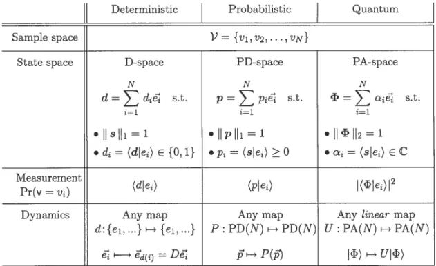
1.6 A Unffied View of Theories
1.6.1 The Vectorial Representation 1.6.2 Variations on the Dynamics 1.6.3 Quantum vs. Classical IVIodels .
12 12 14 16
31
1.6.4 An Algebraic Twist to the Vectorial Representation
CHAPTER 2: CLASSICAL AND QUANTUM THEORIES 0F COMPUTATION
2.1 Deterministic Computation
2.1.1 Turing Machines 2.1.2 Boolean Circuits
2.1.3 Deterministic Complexity Classes
2.2 Probabilistic Computation
2.2.1 Probabilistic, Coin-Flip and Randomised Turing Machines 2.2.2 Probabilistic, Coin-Flip and Randomised Circuits
2.2.3 Equivalence of Probabilistic Models of Computation 2.2.4 Probabilistic Complexity Classes
2.3 Quantum Computation
2.3.1 Quantum Turing Machines
2.3.2 Quantum Circuits
2.3.3 Quantum Complexity Classes
2.4 A Unified Algebraic View of Complexity Classes 93
Characterisations Based on Probabilistic Algebraic Circuits .
Characterisations Based on Reversible Circuits Characterisations Based on Quantum Circuits
Characterisations Based on Extrinsic Quantum Circuits
CHAPTER 3: REAL AND QUATERNIONIC COMPUTING 103
3.1 Real Computing 103
3.1.1 Definitions
3.1.2 Previously Known Results
3.1.3 A New Proof of Equivalence
3.1.4 Further Considerations and Consequences
3.2 Quaternionic Computing
3.2.1 Definitions
3.2.2 Proof of Main Theorem
3.2.3 Considerations and Consequences
CHAPTER 4: COMPLETE PROBLEMS FOR
PROBABILISTIC AND QUANTUM
4.1 Tensor Formule and Related Definitions 4.2 From Gate Arrays to Formule
4.3 From Sum-Free Formule to Gate Arrays 4.4 Completeness Results
4.4.1 The Formula $ub-Trace Problem
4.4.2 Promise Problems and Promise Classes 4.4.3 Promise Versions of the Sub-trace Problem
66 66 66 67 69 72 72 7$ 83 85 88 $8 90 92 2.4.1 2.4.2 2.4.3 2.4.4 96 98 99 101 103 105 107 120 122 122 126 132 C OMPUTING 135 136 140 143 146 146 147 14$
4.4.4 Completeness Results for
Q
andQ
1494.4.5 Completeness Results for the Boolean Algebra IfI 4.5 $ummary of Results and Open Problems
151 152
PART II. DE COMPVTATIONE PER RES QVANTICAS 153
CHAPTER 5: ALGORITHMIC COOLING
5.1 The Quest for Stronger Polarisation
5.1.1 Thermal Equilibrium State
5.1.2 Engineering and Experimental Techniques 5.1.3 Thermodynamical or “Real” Cooling
5.1.4 Polarisation Transfer
5.1.5 Entropy, Data Compression and Molecular “Heat Engines” 5.1.6 Non-Adiabatic Cooling
5.2 Basic Building Blocks
5.2.1 The Basic Compression Subroutine and Its Variants . 5.2.2 Optimality of the BCS
5.2.3 The Heterogeneous Case for 3-qubit Registers
5.3 Scalable Adiabatic Cooling Algorithms
5.3.1 A Very Crude n-qubit Cooling Algorithm 173
5.3.2 Upper Bounds on Cooling Efficiency for Adiabatic Algorithms
5.4 Non-Adiabatic Algorithmic Cooling
5.4.1 The Basic Non-Adiabatic Case: 3-qubit Register
5.4.2 A Truly Scalable Non-Adiabatic Algorithm
CHAPTER 6: EXPERIMENTAL ALGORITHMIC COOLING
6.1 Previous Work and Objectives 6.2 How to Build a Radiator
6.3 A Heat Engine with Three “Cylinders” 6.4 Bypassing the Shannon Bound
6.5 Results and Interpretation
CONCLUSIONS 196 157 157 158 160 160 161 162 166 167 167 169 171 173 174 178 178 180 183 183 184 186 188 191 BIBLIO GRAPHY 200
1.1 Comparison of Deterministic, Probabilistic and Quantum Theories Using
the Vectorial Representation 55
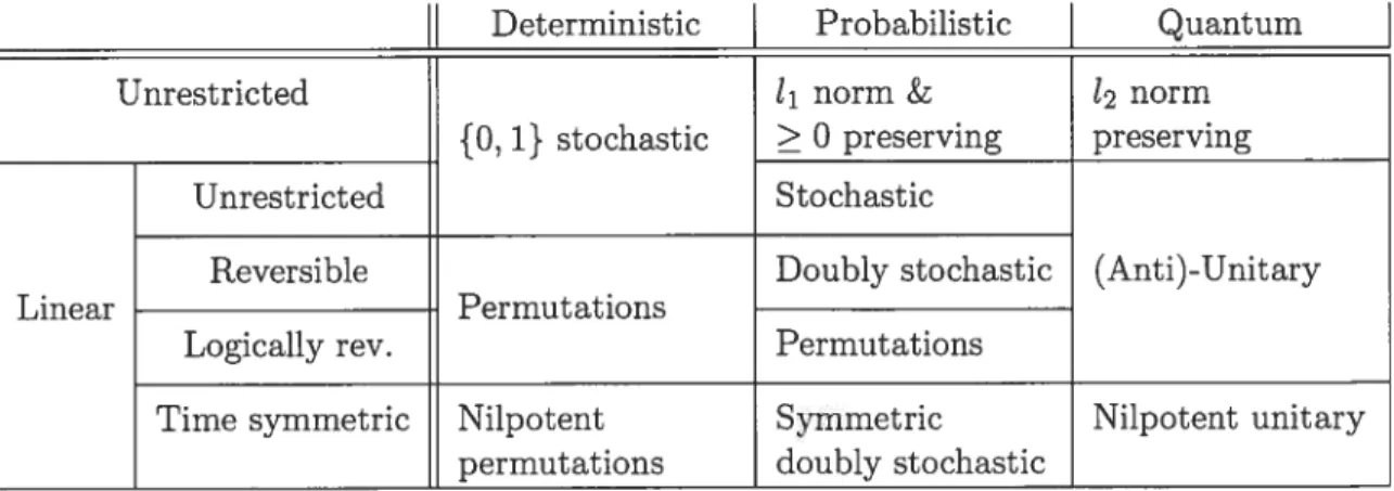
1.2 Comparison of the Dynamics of Deterministic, Prohabilistic and Quantum
Theories 5$
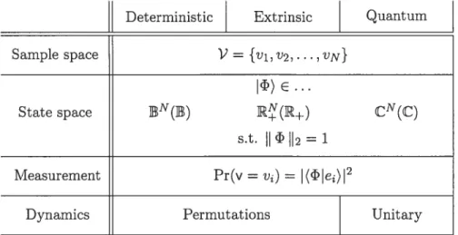
1.3 Common Algebraic Picture for Deterministic, Extrinsic Probabilistic and
Quantum Theories 62
3.1 Resources Needed to Simulate a Quaternionic Circuit 133
4.1 Completeness Resuits $ummarised 152
1.1 Measurement and Dynamics in Deterministic Models 15 1.2 Probabjiistic Models with Deterministic Measurements 23 1.3 Comparison of Probabilistic and Deterministic Models 26
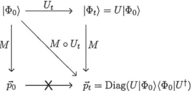
1.4 Commutative Diagram of a Hidden Variable Model 30
1.5 Probability Distributions of a Quantum Model 60
1.6 Complete Taxonomy of Deterministic, Probabilistic and Quantum Theories 65 2.1 Two Equivalent Interpretations of Probabilistic TM’s 76
3.1 Serialisation of a Quantum Circuit 111
3.2 Obtaining a Formula for an N-ary Quantum Circuit 112
3.3 Simulation of a 2-qubit Quantum Gate 113
3.4 Obtaining a Formula for an (N+ 1)-ary Real Circuit 115
3.5 Simulation of a Quantum Circuit by a Real Circuit 115
3.6 Effects of Quaternionic Non-Commutativity on Quaternionic Circuits. . 125 5.1 Basic Building Blocks for the Design of AC Algorithms 169 6.1 Block Diagram of the TCE Non-Adiabatic Cooling Experiment 190 6.2 Detailed Sequences of the TCE Non-Adiabatic Cooling Experiment. . 191 6.3 Result Spectra of the TCE Non-Adiabatic Cooling Experiment 192
Abbreviat ions
• PD. Probability distribution.
• TM, PTM, QTM. Turing IViachine. Probabilistic, Quantum Turing Machine. • NMR. Nuclear Magnetic Resonance.
• QC. Quantum Computing. • AC. Algorithmic Cooling.
Symbols
• Equals by defimtion: =
• Logarithms: log(.) and Ln(.), logarithms in base 2 and e, respectively. • Dirac delta function: cj(j) = 1 if i =
j
and O otherwise.• Kronecker delta: 5jj =
• Statistical relationship: a——b means that the random variable a will take value
b with probability p = Pr(a = b). Also, a—g-.b means that that some object in
state a will evolve to state b with probability p, under some pre-defined statistical transformation.
Typographical Conventions
• Complex numbers: Greek letters, a,
• Quaternions: Creek letters with “hat” symbol, &,
• Conjugation:
— For complex numbers: a — For quaternions: ô
• Measurement variables or random variables: y. • Abstract spaces:
• Vector spaces (modules): V(K), with V being the set of vectors with scalar multi plication defined over the field (or semi-ring, respectively) K.
• Matrices: A
— Matrix transposition: At — Matrix conjugate transposition:
* At, for quaternionic matrices * A, in general
— Ket:
),
a column vector. — Bra: (j, a row vector with(
— n-fold tensor product: A A ® 0 A, n times. — Selection operators:
* (A), - the entry in the i-th row and j-th column of A.
*
(
- the i-th coordinate of .* - the i-th coordinate of çl).
— Trace: Tr(A) for a square matrix A,
— Diagonal: Diag(A), the N-dimensional vector formed by selecting the N di
agonal elements, in order, of an N x N matrix A.
— Identity matrix: I when dimensionality is explicit, otherwise: * I, identity matrix of order x 2
* 12, 13, ... of order 2 x 2, 3 x 3, etc. (subindex a numeral)
• Inner product:
, )
= (xy)• Linear operators:
L
• Superoperators:l’exemple m’a obligé à me traîner jusqu’à la fin, malgré tous les obstacles et la tristesse de découvrir qu’en fin de compte, ça n’en valait même pas la peine
First and foremost, the author wishes to thank his academic collaborators and co-authors, here in aiphabetical order:
Martin Beaudry, $téphane Beauregard, Gilles Brassard,
Markus Hoizer, Raymond Lafiamme, Seth Lloyd, Sasha Mikaelian, Tal Mor, William Schneeberger, Vwani Rowchoudhury, and Yossi Weinstein.
Their participation in joint work, advice and support has been recognised separately in the introduction of Parts I and II of this thesis, along with that of others who have played a significant role in this work.
J’aimerais donc profiter de cette occasion pour proférer des remerciements plus per sonnels.
Tout d’abord, Gilles Brassard, mon directeur. Il m’a fourni le temps, la patience, l’oreille, la liberté, les contacts et le cash, nécessaires pour accomplir cette tâche. Mais c’est surtout comme ami et conseiller qu’il mérite ma gratitude, et le pourquoi, seuls lui et moi le saurons.
À
ce même niveau, Lucie Burelle, mon autre patron, mérite d’être reconnue et re merciée. En plus de me rappeler constamment que c’était temps que je finisse, elle m’a octroyé le temps et la chance de me développer personnellement, ce qui m’a fourni la maturité nécessaire pour finir, ainsi qu’un havre dans lequel j’ai pu me réfugier des frus trations du doctorat pendant toutes ces années.Aussi, Paul Dumais, ancien condisciple à l’Université de Montréal, mérite tout mon respect, car en plus d’avoir réussi à finir plus d’un an avant moi, a aussi développé le module QuCalc pour Mathematica. Sans les adaptations à ce module qu’il a accepté de réaliser pour mieux subvenir à mes besoins, il n’aurait pas été possible de développer NIVIRcalc et ainsi que les autres outils avec lesquels il nous a été possible d’analyser et de préparer nos expériences en résonance magnétique nucléaire. Un grand merci.
Aussi, je tiens à remercier Michel A., Michel J., $teve D. et Louis B., qui ont eu la vision d’embarquer avec nous dans cette aventure et ont été une grande source de motivation et d’appui à tous les niveaux.
Je voudrais également remercier le Très Révérend Père Dom Jacques Garneau et les moines bénédictins de l’abbaye de St-Benoît-du-Lac de m’avoir accueilli chez eux pendant
une période cumulative de près de deux mois. Sans la quiétude que cette isolation m’a fournie, il n’aurait simplement pas été possible de trouver la concentration et la volonté
pour finir cet ouvr age. Je tiens très particulièrement à remercier les pères Beaulieu et
Salvas de m’avoir assisté dans la traduction et dans la recherche de termes scientifiques
adéquats en latin, ainsi que les pères Carette et Leal Martfnez pour leur hospitalité et
accueil chaleureux.
Among my close friends, Laura and Drummond deserve special recognition for their invaluable encouragements and making sure that I remained sane in these last few months. Irina also helped, but to her I am especially thankful for showing me that indeed I might have something to teach, and that I would enjoy doing so, and thus indirectly providing an indispensable source of motivation to accomplish all of this and make it to
the end.
Mes futurs collègues de l’École Polytechnique de Montréal (tout particulièrement Sa muel Pierre pour ses encouragements et Pierre Robillard pour sa patience) ont sans le vouloir jouer un rôle fondamental dans cette dernière année : ils ont fourni un condi
tionnant positif sans lequel je me demande encore si
j
‘aurais trouvé la motivation pour finir.D’un autre côté, je dois aussi reconnaître et remercier mon épouse Sandra, qui après
toutes ces années a fini par comprendre comment et pourquoi il fallait que ça prenne aussi
longtemps. Mais aussi, parce qu’elle a été sans le vouloir la source de conditionnement
négatif tout aussi nécessaire pour m’avoir poussé à terminer.
Et finalement, ma mère Anne-Iv1arie qui pendant tout ce temps m’a soutenu à tous
les niveaux (y compris la soupe). Mais aussi car je suis pleinement conscient de tous les sacrifices qu’elle a réalisés pour ce doctorat devienne une réalité, récemment, mais aussi il y a longtemps.
About Computation...
Thus is the nature of the game in Theory of Computing and Complexity: We look at the different modeis which could be built, in principle, to see if they are equivalent. If they are the physics or engineering are of no concern, and can be “abstracted away” If they are not, then we know what features are worth worrying about. As a result of playing this game, with many possible models, the two following principles of the Theory of Computing have been postulated:
• The Church-Turing (CT) Thesis: Ail models of computation that we can propose are either weaker or equaily powerful to the so-caUed universal models of com putations, of which the historicaily most significant are the Turing Machine and Church’s Lambda calculus.
• The Strong Church-Turing Thesis: 0f ah modeis that we can propose, none is fundamentaily more efficient than the above.
However, here we have the theory of quantum computing, which thumbs its nose at the Strong Church-Turing thesis. In appearance, it seems that the thing quantum does help computation as it seems to allow to compute things more efficiently with it than without. So, if we are willing to believe that such a beast as a quantum computer couid be built, it seems that the Strong CT Thesis could go the way of the theory of the ether...
About Quantum Physics...
But what is this mysterious thing quantum? What is its essence? The term “quan tum” is a Latin adverb meaning “as much as,” and has the same root as “quantity.” Historically, in Physics, it had to do with certain physical quantities being “quantised,” or more preciseiy discretised. Energy, in particular, a continuous quantity in Classical Physics, is discretised and one speaks of “quanta of energy”. Beyond the mere name, lies a new paradigm for the description of physical reahity and its dynamics, with a new and axiomatic mathematicai formalism describing it.
As a doctoral student with no Quantum IVlechanics background, I was damned if I was going to iearn the physics. So I had to exorcise the daemons of Physics out of
quantum computing, before I could understand it, let alone do research in it. Demons
such as “Observables,” “Borel sets,” “Hamiltonians,” “infinite-dimensional space,” and a menagerie of other weird animais, such as cats who cannot make up their minds, fermions
that can’t stand each other, bosons that do, etc, etc.
More to the point, Quantum Physics was introduced at the turn of the last celltury
to heip solve sorne of the mysteries physicists were facing then (photoelectric effect. etc.).
However the mystery that I (and many others) face as a computer scientist is quite
another. About this thing quantum which aids computation, we must ask the following: what in it is essentiai in the context of computation, and of these properties which are the ones at the origin of the demise of the strong CI thesis?
About the thing quantum which accelerates computation...
Fortunateiy, by the time I started my Ph.D. the exorcism was weli under way. The quantum circuit abstraction was already the king of the hiil. A simple model which under
some quantum equivaient of the strong CI thesis (or rather, a patched version replacing it) is beheved to be equivaient to ail other models quantum. It is an important fact that not ail of die axioms of Quantum Mechanics (as it is usuaily defined) are reievant in
the context of computation. Thus, when we speak here of the thing quantum, we are
aiready considering a subset of the properties of “quantumness” of physical reahty. A lot of the “demoniacal” characteristics of Quantum Physics (space, time, energy, etc.) can and must be abstracted away, which is what the quantum circuit modei achieves.
Another non-negligibie positive side-effect of adopting that model is that it also exorcises
many of Computabihty Theory’s own idiosyncrasies, with which a dose of the quantum
thing becomes monstrous.1
A first impression of mine was that in quantum computing, quantumness had httie to do with quantities being “quantised” (yech! what an awful phrase...). As a matter of fact,
things are aiready quantised in computation: it is a fundamentai tenet of the Theory of Computing (which supports both the weak and strong Ci theses), that under reasonable assumptions 2 ail quantities can be quantised, i.e. digitised. without ioss of generahty or ‘Indeed, much like the effect of an after-midnight snack on a peaceful Gremiin, the resuit of feeding some quantum tape into an unsuspecting Turing Machine is not a pretty sight. The poor thing becomes
so confused and agitated that it cannot figure ont when to stop! Kids, do flot try this at home, unless
you want to spend the rest of your Ph.D. figuring out when or how it is going to hait and go back to its
normal, peaceful self...
power of computation. So. we can forget about looking at the Latin dictionary for more dues.
Having thus extracted the essential, which of the remaining properties of quantum
computing are responsible to create that difference, to assist computation? The first sus pect is its time-symmetry or reversibility, linked to the unitarity of the allowed dynamic transformations in Quantum Physics. However, that is clearly not it (it is a restriction!),
as again reversibility was shown to be a requirement which does not restrict power, i.e.
the strong CT stili holds under it.
Quantum parallelism is another popular one. It has to do with the ability of a system
or computational device to mysteriously “be” in several states at the same time. Or
with cats which are not content with their seven lives, but also want to have a few deaths as well... IViore seriously, it can be modelled by replacing the set of configurations
of the computational device (its states) by a richer set which includes suitable linear combinations of the elements of the old; thus, non-trivial linear combinations represent
these “mysterious” parallel states. That could be it, but early on it was pointed out to me that no, that was not it in itself. This property is essential, yes, but not a priori
sufficient.
In fact quantum parallelism unbridled can lead to models of computation which are unreasonably powerful (a phenomenon similar to that of analogue computing...). What
provides that modulating restriction on the model is the inability to obtain total infor
mation on these new states of a computational device. This restriction is given by a
measurement mule or principle. which in some sense says that the nice mathematical trick we have pulled by replacing the state set by a linear space is very nice and clever, but
useless in the end: our observations are stiil bound to and based on the original state set, which we often refer to as the computationat basis of the linear state space. This
principle is, in some sense, the computational equivalent of the principle of quantisa
tion in Physics. One can sa that even though the linear state space is “continuous”
(it does form a complete metric space), the quantities representing measurements on it
are “quantised” in that only a finite (albeit exponentially large) number of “values” (the base states) can be observed. Thus, with this tenuous epistemological link, we renege our initial impression that there was nothing “quantum” about quantum computation... Given this restriction, I was told, what is necessary for this thing quantum to pro computing are not covered by the strong CT thesis, but these models are considered unreasonable due to the impossibility of constructing devices with arbitrary precision and accuracy.
duce interesting resuits is the abillty for these parallel existences to cancel each other in some cases; a phenomenon referred to as interference. At that tirne, it was already
intuitively perceived that it was this property of quantumness which is esseutial, as with out this property the known, interesting quantum algorithms wouid cease to work. This is flot only true of computation, but of quantum mechanics at large also. As Feynmann,
thinking about Physics rather than about computation, had already put it, “somehow or other, it is as if probabilities sometimes needed to go negative.” How does one, however,
carefully enunciate, let alone prove, such a principle?
Because these things are hard, it was not my intention to go about formalising siich a principle. However, it happened, by accident. $o, how does one go about it? “Go back
to principles,” the old adage says. And indeed we go back to the nature of the game in Computability and Complexity Theory, as we described right at the beginning: we define
new models, we see if they are equivalent.
First, we will play this game with the intent of narrowing down what that thing quantum really is, from the computing point of view. We will build a “unified” model of computation or meta-model in which we can describe ail the usuai models (determin istic, probabihstic and quantum), and even some new ones. These modeis will ail have
the same structural properties of parallehsm (iinearity of the state space) and the same
measurement principies. In this meta-model of computation, we have a single varying
parameter which instantiates the different modeis: the algebraic structure on which the
iinear state space is defined. This structure wiil define the allowed coefficients in linear combinations of base states, coefficients which, due to their relationship wit.h the mea suring mies, are often cailed pro babitity amplitudes. Since the oniy thing that changes is this underlying algebraic structure, we cali this method the atgebrazc approack.
Using this method is a good idea, firstly because it provides a nice “big picture.” Secondly. it provides us with tools for proving the equivalence of some of these mod els. Thus, we can build a “hierarchy” of modeis (or compiexity classes) based on this
parameter. Some leveis collapse, some we do not know. More concretely. and coming
back to our main question, on that hierarchy we wili be able to draw a une, a frontier, beyond which things can possibiy vioiate the strong CT thesis. In particular, quantum computing, as usuaily defined, is beyond that une, and classicai and probabihstic on this side of it. This une, this separation, corresponds precisety to what we thought it was, this is, paraphrasing feynmann, that abihty for probabihty amplitudes to become negative,
and hence with the possibility annulling each other.
Unfortunately, while Te strongly believe that this une is ‘for real” and not just an illusion or a product of oui’ own mathematicai ineptitude, there is to this day no solid
proof of its existence. Even though we can solve surprisingly hard prohiems within the quantum model, there is stiil no formai proof that these problems could not be solved under more traditional models3. With respect to this question, a third, albeit marginal, advantage of this meta-model is that it seems to bring us doser to resolving that question. In fact it gives a target to shoot at. Along with that une cornes a complete problem for the quantum model, which we can try to show outside of traditional complexity classes. At the heart of the problem is the necessity to keep track of the signs of the amplitudes in order to correctly simulate the final probabilities of measurement. The apparent inability of classical probabilistic algorithms to do so provides some “evidence”, as a complexity-theorist would put it, that there is a non-empty gap between the probabilistic and quantum models.
About computing with quantum things...
In, theory. there is no difference between theory and practice.
In pTactice, there is...
Thus quoth the Computer Engineer to the Theoreticai Computer Scientist4. To this
the computer scientist can respolld in a variety of ways. If he is ahie to do so, he will go
back to the whiteboard and prove that these differences are insubstantial to the power of computation of the device being built. He then hits the engineer right back with
the aimighty CT thesis, in its appropriately patched, hard cover version, saying “No, there isn’t.” If he is generous enough, he might provide the Engineer with a proof of
that statement, which she can hopefully make into a simulation method of the original theoretical model bv the device.
0f course, if the computer scientist does not succeed to prove it (either because
he is too stupid, or because it is simply not true), then he will create a new, revised theory, write it up and present it to the Engineer, nonchaiantly saying “Now, there
3More precisely, the only exponential complexity separations between the classical and quantum mod els that have been shown are for the query complexity of certain computational tasks; no such separations
have been exhibited in terms of absolute complexity measures (e.g. time or space). 40r, for that matter, SO can the physicist in the context of quantum computing.
isn’t.” Nodding lier head, the Engineer will ask, “So what of the old theory? Does this mean that we cannot compute what we wanted to?” And so on...
This is exactly the situation that has arisen in the field of Experimental Quantum Computer Engineering. $o far the most successful technique for implementing small-scale quantum computations is that employing the principles of Nuclear Magnetic Resona.nce. This method utilises the magnetic spins of a macroscopic sample to represent quantum bits (called qubits), and employs an NMR spectrometer to manipulate and read out this collective magnetisation. In theory, this method is a correct implementation of the quan tum model. However, this is only so under conditions which cannot be achieved today and might neyer be easy to achieve. Thus in practice, and if we restrict ourselves to NMR, there is a difference between what we can do and what we would like to do, theo retically. More concretely, the two main deviations of NMR QC from the garden-variety quantum computing model are a) a different measurement mie, and b) the inability to initialise the computation with a pure state, or in other words the inability to reset the memory to a known state before starting the computation.
In this case, the first reaction of the theoretician corresponds to trying to show to the experimentalist that these shortcomings will not make a difference in the power of computation of his device, hence providing an extended version of the strong “quantum” CT thesis. $o going back to the beginning once more, we, theoreticians, define revised theoretical model and try to show them equivalent or inequivalent to the previous models. So far, we have been unable to do so. In fact, even the time-tested technique of Divide and Conquer, a favourite of many Theoretical Computer Scientists, does not work here: we do not know how to show the equivalence of these models (or lack thereof) even if
onÏy one of these discrepancies is introduced.
Ultimately, since we cannot conclusively answer any of the questions of the Engi neer/Experimentalist, what is a theoretician to do? One answer is to become an experi mentalist ourselves and try to solve some of these problems at that level, and make some of these differences vanish. 0f course, there are limits on how “wet” most theoreticians will get their hands...
To solve the problem of initialisation, one very interesting theoretical resuit of an “ex perimental” nature is the discovery of the technique of algorithmic cooting. In its original variant, it consists in performing a pre-computation prepamation of the memory, such as the result a small portion of it is in a known state. This purified portion can then be used
for the intended computation. This process is in fact a kind of compression algorithm, whose action eau be viewed as lowering the entropy or associated “temperature” of the purified portion of the memory; hence the name. The price to pay is that the remainder of the memory cannot be used. Furthermore, the size of the purified region is limited by how mixed the states are initially, and is far too small to make a difference with current experimental technology. So, while the idea is nice in theory, it is not in practice.
What is ironic, is that that these techniques had long been known under the name of potarisation transfeT by NMR spectroscopists. While some interesting theoretical resuits providing limits on the efficiency of these techniques were known, as far as we know true compression experiments had not been performed, nor had true scalable algorithms for arbitrary-sized memories been described.
A second improved variant was proposed which in principle could be made practical. It involves recycling the wasted part of the memory by interaction with the environment. This process, called thermatisation, allows those bits to go back to their initial state, and then to be used again to purify another region of the memory with the same compression algorithms as before. By combining compression and thermalisation, and under the right conditions, it is possible to purify the whole memory. We present here a new and more practical method of doing so, achieving satisfactory levels of purification, even with initial states such as those encountered with current technology. We also study the fundamental limits of such techniques, in thus extending those results known about the first variant.
Unfortunately, these methods require ideal conditions which are not easy to obtain in the lab. In particular, we must have that the purified part of the memory be completely isolated from the environment, or alternatively that the length of the thermalisation process be very short compared with the time it takes for the purified part to go back to its natural mixed state.
Wanting desperately to get my hands wet, the objective I set myself vas to actually perform a proof-of-concept experiment demonstrating this method, or at least a simplified version thereof. The first step was to analyse which were the threshold conditions which had to be attained in order for the experiment to work, in particular which was the minimal gap between thermalisation times of the purified portion a.nd the portion to be recycled. Once these minimal conditions were established, an experimental technique had to be found in order to achieve those conditions. We were fortunate to find and perfeet a chemical laboratory technique that allowed us to manipulate just enough these
thermalisation times, The experiment was successful (barely), thus accomplishing two important objectives: a) proving that algorithmic cooling cari work even in the lab, and b)
proving that if a mere theoretician can make it work, surely professional experimentalists can improve it to make it even more practical. So there!!!
De adhibenda re quantica
About the quantum thing which acceterates cornputa.tion
\rhat is indeed the nature of this thing quantum which appears to make computations
using it go faster? Is it entangiement, is it state superposition, is it interference of
computationai paths? This question lias puzzled researchers in Quantum Computing in
its beginnings, but it is now generally understood that the key ingredient without which no speed up eau occur is interference. In this first part of the thesis we have sought to make that intuition as formai as possible.
Chapter 1 introduces a mini-epistemology of deterministic, probabilistic and quantum
theories. We make tabula rasa of ail previous axioms and principles of these theories, in particular Quantum Mechanics, and painstakingly re-introduce only those character istics of these theories which are relevant and non-redundant. The prize is a uniform
mathematical model, based on vector spaces, within which we can uniformly describe the models of these theories, in particular computational modeis.
In Chapter 2, we review the standard models of classicai and quantum computation, however, presenting them, in some cases, in a more generahsed fashion. In particular, we develop a notion of circuit more general and formai than the one usualiy introduced, which wili aliow us to define circuits operating and computing with states defined on
arbitrary aigebraic structures. This will in turn allow us to characterise the most impor tant compiexity classes. both classicai and quantum, within a unified framework. whereby
variations in the underlying state structure plays a centrai role in generating the richness and variety of the compiexity picture.
In the iast two chapters of this part, we go beyond mereiy restating what vas known in more formai terms. In Chapter 3, we compiete the aigebraic picture of complexity classes by considering the quaternionic numbers. We ask and answer the question of which complexity class(es) they generate. Finaliy, in chapter 4 we use the formalism of tensor formule to strengthen the abstract classification of Cliapter 2 by providing a family of complete and promise-complete prohiems for tlie relevant classical and quantum complexity classes.
Credits and Acknowledgements
The work in Cliapters 1 and 2 is mostly a straightforward formalisation and gen erabsation of previously introduced concepts. Pew novel resuits are to be found tliere, except maybe for tlie proof that no models other than deterministic ones exist which are
simultaneously quantum and probabilistic. This is joint work with Michel Boyer. who generalised an earlier resuit of the author. This whole question was born in discussions with David Poulin.
The resuit on quaternions in Chapter 3 is joint work with William Schneeberger, who should be credited with the main idea. The author was only responsible for working out the details.. .
The contents of this chapter are alrnost exactly the same as those of our joint article on this topic [FSO3]•
finally, the notion of a strong characterisation through complete problems based on tensor formula was born in conversations with Markus Holzer while he was a postdoctoral fellow with Pierre IVlcKenzie at the Université de Montréal. These ideas were painstak ingly developed by Martin Beaudry, from the Université de $herbrooke, in a long and slow process, whose results are gathered in a joint article [BFH02], on which Chapter 4 is largely based.
In addition to my co-authors, the following persons played a crucial role in discussions, to motivate and validate (not always agreeing...) the work of the author in these topics: Lance Fortnow, Michele Mosca, David Poulin and John Watrous.
A THEORY 0F THEORIES
“Vade retro Satanas!”
1.1 About Theories and Models
From a scientific point of view, a theory is the set of abstract principles, axioms, and hypotheses that have been formulated with the objective of describing a reality, and
ultimately make predictions about it.1 The axioms and rules of a theory allow us to construct models of reality. These models allow us in turn to describe, understand and,
hopefully, accurately predict the behaviour of the particular siiver of reality that the
theory strives to encompass.
Que central dogma of modem Epistemology is that no theory is perfect nor can it be. Reality is just too big and complex for our feeble littie minds. Independently of
whether we want to accept this philosophical principle or not, the practical reality is
that sometirnes a theory of everything is just too cumbersome. Whether by necessity or
by choice, our theories remain abstract and factor away those aspects of reality which we cannot grasp or we choose to ignore. For example, the PTincipte of Abstraction has
become in Modem Science and Engineering a maxim indoctrinated into beginners and a universal methodology:
Ignore everything that witt not affect your predictions.
In the sciences and engineering, the models that a theory allow us to construct de-scribe systems. which are the limited portions of reality which we wish to understand. The state of a system is the abstract object that describes it. From it depend the resuits of measurements, which lis how information can be extracted about the system from
‘The Oxford English Dictionarv[OEDS9] gives the following definitions of theory in this sense:
a) a scheme or system of ideas or statements held as an explanation or account of a group of facts or phenomena;
b) a statement ofwhatare held to be the general laws, principles, or causes of something known or observed.
and the Webster c03]
as:
without. finalhç the dynamics of the theory prescribe how the states will change and evolve with time. 2
As unexpected resuits are obtained or as phenomena unexplainable under the current theories are observed, we formulate new theories or revise old ones. That has tradition ally been the pattern in the Natural Sciences. However, in the Applied Sciences and Engineering it is often that some of the aspects that we had previously neglected or abstracted away become of interest. Thus, theories can become partially obsolete ont of io fault of their own, but out of the fact that they no longer meet our changing scope of applications.
Furthermore, according to the relativism mentioned above, different fields of knowl edge contribute complementary aspects of the understanding of reality. Physics and Computer Science have provided in the last thirty years one remarkable example of how these points of view can meet and enrich each other. The field of Quantum Computing is indeed one the chiidren of this happy marnage.3
In the end, and for whichever reason, the fact is that there are many valid and worthy theonies, each with their own utility and scope of application. Indeed, their variety and number make it useful to study them systematically, identifying their common features and classifying them according to their differences. In other words, to define an epistemological theory of theories. Not a theory of everything but one limited to physical theories and theories of computation. one that will suit our particular purpose.
The types of theories that will interest us in the context of Physics and Computation are deterministic, pro babitistic, and quantum theories. But befone we start enunciating what they are, a word about nomenclature. With the advent of Quantum Computing, the traditional Theory of Computation, i.e. the deterministic and probabilistic models of computing, have been re-dubbed the ctassical Theory of Computation. A similar phenomenon has occurred in Physics where nowadays the term “classical” is used for those theories which are neither relativistic nor quantum. However, there might be some ambiguity about whether probabilistic theonies should be considered classical. Some scientific texts and historians of Science. especially older 011es, stili refer to Classical Physics as that of Newton and its successors, excluding Statistical Mechanics. In the rest of this document, we will abide with the more modem use in both Physics and the 2When we say that states evoive with “time,” we do flot necessariiy meanphysicat time, avery shppery business... It is only under very specific circumstances that computational time can be equated to physical time.
Theory of Computation.
1.2 Deterministic Theories 1.2.1 Concepts and Definitions
In classical deterministic theories, the notion of state unequivocaily defines with ab solute precision ail of the attributes and properties of the system. From the knowledge of
the state of a system, ail predictions are deterministic and the answer to every possible question or resuit of every possible measurement at that moment is uniquely defined by
the state object. Furthermore, the dynamics of a deterministic theory is such that given
its initiai state, the state of a system at any future moment is uniquely defined, and thus so is the outcome of ail possible measurements in the future. These are in fact the two axioms of a deterministic theory.
Definition 1.1 (Deterministic Theory). The axioms of Deterministic Theory are the
following:
Axiom 1 (Measurement Rule). The state of a system preciseiy and unequivocally defines the resuits of ail possible measurements.
Axiom 2 (Dynamics). How systems evoivewithtime depends exclusiveiy on the prop
erties of these previous states of the system, whether measurement related or not. For simplicity, and without loss of generaiity, we xviii assume throughout that the resuit of ail measurements can be represented with a single variable defined over a unified outcome domain. In that case, we can then give the foiiowing formai definition.
Definition 1.2 (Deterministic Model; Deterministic Theory). A deterministic
modet is a 4-tuple (8, V,
f,
V) comprised of the foiiowing elements: • 8 is the state space,• V is the set of resuits of ail measurements.
• f
: 8 t— V is the measurement rute, where f(s) represents the outcome of measurement on state s
e
8, and• V {D(t1, t2) : 8 i—# 8} is the famiiy of evoiution functions parametrised by valid
times of observation t1 < t2. such that if the state of the system at t1 is s, then the state of the system at time t2 is s = D(ti, t2)(si).
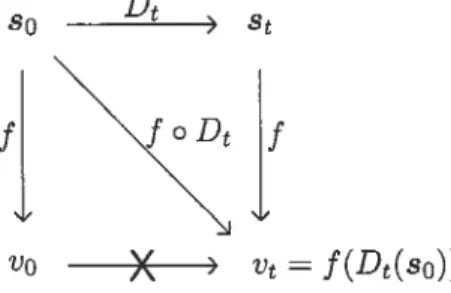
To sirnplify our presentation, let us represent the outcome of a measurernent at time t with a single variable v(t). Alsot, let D : S S represent the tirne evolution function from some fixed initial time to to a later tirne t > t0, Le.
D = D(to, t) (1.1)
A very important characteristic of deterministic models is that it is aiways possible to make a deterministic prediction of the outcome of measurement. In particular, given
the initial state o at to, it is possible to infer the value of v(É) as follows
v(t) = Vt f(D(so)) (1.2)
However, what the dynamics does not define is a rnap between measurernent outcomes
v and Vt at times t0 and t respectively. In other words, given onty knowledge of vo, we
cannot determine with certainty the value ofVt. This situation is described in Figure 1.1.
) st
vo
X
> Vt = f(Dt(so))Figure 1.1: The relationship between states and measurement outcomes in deterministic models. The crossed-out arrow indicates that no deterministic relationship exists.
The non-existence of a deterministic time evolution map between measurement out
cornes stems from the fact that there rnight be more than one state with the same outcome, or in other words that
f
is not a bijection. Suppose that we could only observe a system at one fixed moment in time. Then, all states s of the system with the same measurernent outcorne would appear indistinguishable to us. In fact, the measurement rules define an equivalence TeÏation in the state space S, where each equivaience class[s] = {s’
I
f(s’) f(s)} represents all the states which are rnutually indistinguishable.In the absence of knowledge on the dynamics or because of the inability to re-measure
at a later time, this indistinguishability is complete. That is why these equivalence
1Whule it is true that in most physical theories. the time evolution functionD(t1,t2) will only depend
classes are sometimes called partial information states or also macro-states (also written as M-states), in contrast with the original states which are dubbed total information
states or mzcro-states (or t-states). is equivalent to considering a model with a new
state space
57f,
the quotient of S under the relation deffned by the measurement fuief.
The state space 57f is in fact isomorphic to the space of measurement values V adopted
by the total measurement variable y, with each value y being associated uniquely with an M-state[s] as follows
e [s] f(s’) = e for some s’ [s] (1.3)
Because there is no deterministic map between outcome values, unfortunately such a model would not be deterministic, as there would be no deterministic map between IVI-states.
1.2.2 Examples of Deterministic Models
In the rest of this section, we will introduce and discuss some examples of deterministic models relevant to our purposes.
1.2.2.1 Turing Machines
The quintessential exampie of deterministic models in the Theory of Computation
is the Turing Machine, an abstraction of computationai devices which according to the Church-Turing Thesis embodies the essence of all imaginable and reasonable computa tion. It consists of a finite state machine or automaton, an infinite memory tape (with a beginning and no end) consisting of individual cells, and a read-write tape head con trolled by the automaton that can move to any position on the tape, but only moving by one cell at each step. In one of its simplest formulation, the Turing Machine tape contains only binary input symbols in = {O, 1} and blank celis, represented with the
symbol . In other words. the tape alphabet is F U
{}.
In that case. it can then be formally defined as follows:Definition 1.3 (Turing Machine). A Turing Machine (TM) is a 4-tuple,
(Q,
q, q,S) where• qo E
Q
is the initiat state of the automaton.• q E
Q
is the final or haïting state of the automaton.• 6, is the transition function describing the beha.viour of the 1M, where
6: Q—{qf} x F i’ Qxfx{L,R}.
The image S(q,b) = (q’,b’, d) indicates what the TM wili do next when the automaton
is in internai state q E
Q,
q q, and the symbol under the tape head is b. First, it willoverwrite it with b’. Then, it will move the head in the direction indicated by d: right if d= R, left if cl = L, and stationary if cl = L and it is at the beginning of the tape. Finaily,
the internai state of the automaton wiil change to q’. Upon entering the final state q, the TIVI wili haït and perform no further action.
States. At any given moment of the computation, the state of a 1M, also referred to as its configuration, is defined by the state of its internai finite automaton, the position of the tape head. and the svmbols written on its tape.5 Configurations are typicafly
represented by a string [CL,q,CR], where q is a string representation of the internai state of the automaton. CL E P is the string of tape symbois to the ieft of tape head, and CR E F* is the string of symbois under the head and to its right up to the iast non-biank symbol. The configuration string is thus aiways finite.
Dynamics. The dynamics of this model is defined by the transition function 6 and the
fact that the TM will hait upon entering the final internai state q. It is therefore fuiiy deterministic.
Measurement. According to the spirit of the modei, what can be “seen” of a Turing Machine hy an external observer are its tape contents, its tape head position and whether the machine lias haÏted. More formaÏÏy, that means if the TM is in configuration [CL.q, cRi.
then the resuit of our observations can be represented as [CL,h,CR], where h is a Booiean variable representing whether q = q.
51n the Theory of Computation. the term configuration is used to distinguish the state of the 1M with the state of the internai automaton, a system within a system. Here we use the term state for the
However, nothing fundamental in the Theory of Computation prevents observation of ail the components of the state of a T\i, including the internai state. In fact, this allows for the principle of simulation in which a 1M or another kind of computational device mimics the behaviour of a TM by observing and keeping track of its successive configurations. One of the consequences of the Universality Theorem for Turing Machines is that computability is not affected. nor is problem compiexity (for most reasonabie classes), by whether we adopt thiswhite box model or the more abstract black box model
just mentioned. Consequently, the resuits and predictions of the underlying theory are not affected whether we allow full or only partial observation of the 1M configurations, or in other words on how we define macro-states as long as they include the contents of the tape.
1.2.2.2 Boolean Circuits
Bootean or togicat circuits were invented as an abstraction of electronic circuits, today ubiquitous even within the computer on which this text is being written. Thev consist of elementary logical gates operating on Boolean variables which are ‘brought” to them by wires which interconnect the gates. Ihese Boolean values (O or 1) are idealised abstractions representing some physical property such as voltage. The gates operate on these values
Abstractly, a circuit can be defined as a graph with the following properties:
Definition 1.4. A circuit C = (I, O, Ç, W) is a special kind of directed acyctic graph (V, W) with vertices V and edges W, where
• The set of vertices is partitioned into three components V = IUOU Ç, where
— I represents the input nodes, to which a given “input” value is assigned at
initialisation.
— O represents the output nodes, from which the “output” of the circuit will be
determined.
— Ç is the set of gates in the circuit, each transforming the values on its input
connections onto values on its output connections according to a fixed rule. • The set ofedges W
c
(IuOu(Ç
x N)) x (IUOU(Ç x N)) ofthe graph. corresponds to “wires” linking input and output nodes with the (labelled) connections of the gates, with the following restrictions and semantics. If w = (u,y)
e
W then:— u E I and t = (g.
j)
E Ç x N, indicates that the u-th input node is connectedto the j-th input connection of gate g E Ç
— u E O and u = (g, i) E Ç x N, indicates that the i-th output connection of g
is connected to the v-th output node
— u, u E Ç x N, with u = (g, i) and y = (g’,
j)
indicates that the i-th outputconnection of g is connected to the j-th input connection of gate g’.
— u E I and u E O indicates a direct connection from an input node to an
output node, without going through any gates.
— the in-degree of any input connection or output node is 1 (no fan-in).
Intuitively, circuits are used as computing devices by setting the input nodes to the input of the computational task we want to solve. The values then “propagate” to the input connections of ail connected gates through the wires of the circuits. These gates in turn act by “reading” ail input connections, and “writing” the correct values onto the output connections, which are in turn propagated to the next gates or output nodes. The output of the circuit is defined when ah output nodes have “received” a value, and consists of the combined values of all output nodes.
In particular, a Boolean circuit is one where all the gates g implement a fixed logical operation such as AND, OR or NOT, or ntore generally any map g : ‘‘ where k and
/ are the number of input and output connections of g, respectively.
As an example of a deterministic model, Boolean circuits have the following elements.
Measurement. The interface with the outside is defined by the output nodes. Their values are the observables of the system and their value is aiways uniquely defined.
States and Dynamics. If viewed as a physical system, the state of the circuit could be defined as the collection of Boolean values that each of the wires of the circuit has. However, such a description is not very useful as it represents the complete computation, from input to output, and from beginning to end. We would like to require the notion of state to correspond to a particular moment within the computation. However, in circuits
the notion of time becomes somewhat elusive and unconventional.
There is no implicit notion of time as a motor of change in circuits: change in a
circuit is effected by the gates. Whilst a notion of “before” and “after” can be defined within each gate, the fact is that the graph of wires interconnecting the gates does not
necessarily define a unique total ordering of the gates themselves. As a consequence, in some cases saying that this gate was “before” this one can be meaningless.
What are these “moments” then, at which it is sensible to define the state of circuit? They can modelled as bipartite cuts in the circuit graph with certain particular properties. Definition 1.5 (Temporal Cut of a Circuit). A temporal cut of a circuit C is a
bipartite cut (Ç,, Ç) of the circuit graph (i.e. Ç, fl Ç 0 and Ç, UÇa = V), where we
cali Ç, the “left” side and Çp. the “right” side, with the following properties:
i. Ail input nodes are on the ieft side, and ah output nodes are on the right side, i,e.IC Ç, and Oc Ç.
ii. All wires across the cut are directed from the left to the right, i.e. there are no
w= (‘u,y) e W such that u E Çp. and e E Ç,, we
The width of a temporal cut is the number wires that cross the dut, i.e. {w = (u. e)
I
u e Ç, and e E Ç} 6Let 7 be the set of ah temporal cuts of a circuit C. We can define a partial order
within 7 as foilows
Definition 1.6. Let t = (Ç,,Ç) and t’ = (Ç’,, Ç’a) be two temporal cuts in 7. We say
that t < t’ if
a) (Immediate successor.) Ç’, = Ç. U {u}, where u é Ç, or
b) (TTansitivity.) There exist., ti.... ,tm E fb, m 1, such that t < ti < < trn < t’. With this definition, we can properly identify the “initial” and “final” moments to and
tf as the cuts cutting all and only the input wires (Ç. I) and that cutting all and only
the output wires (Ç = O), respectively. In particular, we will have that to = min(fa’)
and tf = max(Tc). We can thus view T as a computational equivalent of the space-tirne
continuum for C. However, 7z is not totally ordered and therefore there is no unique “trajectory” of time, or in other words no well defined time “axis.”
If we really insist on having a “proper,” fully ordered notion of time, we cari aiways
choose one hy making arbitrary choices or by incorporating into our model other elements of reality which would make that choice for us. For example, if we were to attribute 6Note that the situation is somewhat simplified ifweconsider reversible circuits or gate arrays,where
lengths to the wires then it would be possible to define a sensible temporal ordering of
the gates in the graph, associat.ed with the physical events of voltage change at each of the gates, where the initial moment corresponds to a simultaneous change of voltage in
ail the input nodes.7
Regardless, these temporal cuts can also be intuitively viewed as moments at which one of the many correct simulations of the circuit could have stopped. Thus, it is sensible to associate to each possible cut a state of the circuit at the corresponding moment.
Definition 1.7 (State of a Boolean Circuit). The state of a boolean circuit G at a temporal cut t = (Ç,
)
of width m is the vector of boolean values (b1, b2, . ..,where for 1 <i <ra, b E lI is the wire value of the i-th wire w= (u, e) crossing the cut
(according to some arbitrary ordering of the wires).
In particular, the states associated with to and tf are called the initiat state and the
final state, respectively.
The dynamics of a Boolean circuit can be deterministically described in terms of its
gates and its states as follows. Let s be the state at a cut t, and let cutt’ be an immediate successor of t, i.e. Ç’ = Ç U {g}, where g E Ç is a gate of the circuit. The state s’ at
time t’ is constructed by taking the entries corresponding to the input connections of g. and substituting them with the values of the output connections as defined by the truth table of g and the values at the input connections. In general, and by applying
this method iteratively, it is thus possible to uniquely determine the state of the circuit
at any moment t’, given a description of the state of the circuit at any moment t < t’ that precedes it.
1.2.2.3 Classical Mechanics
In its Laplacian or Hamiltonian formulations, Classical Mechanics is also a determin istic theory.
States. It is sufficient to consider the position and momentum vectors for ail particles
in the system. Thus, states can be represented as the set of ah 3-dimensional coordinates of the position and momentum vectors with respect to an initial frame.
TBut that is precisely the kind of model that would violate our cherished Principle of Abstraction, as
these lengths would in no way change the ultimate outcome of the computation, which is why we do not
Dynamics. The dynamics of such systems is represented by the Laplacian or Ramil tonian operators. From them. and given an initial state, it is always possible to uniquely determine the state of the system at a later time t. In other words, there exists a de
terministic map D on the state space S, D : S F—> S, such that St = Dt(s) is the state
of the state description of the system after time t lias elapsed from the system being in
state s. In this case, D only depends on the Hamiltonian/Laplacian of the system and
the elapsed time t.
Measurement. Nothing fundamental in this theory prevents ns from obtaining full in formation on the exact value of these coordinates. Measurements are, in principle, fully
unrestricted. This would be tantamount to equating micro-states and macro-states. Un
der more reasonable circumstances, however, observations are restricted to macroscopic variables such as speed and position of the centre of mass, angular momentum, etc. In this case, macro-states are equivalent to the Cartesian product of the domain of these variables.
1.3 Probabilistic Theories
1.3.1 What Is a Probabilistic Theory?
In our objective to trim our meta-model of theories to the bare essentials, let us forget for a minute everything we know or might know about probabilistic models, and adopt
a nescient approach. First, and by their name, we can assume that they somehow must
involve probabilities, an otherwise abstract mathematical concept defined axiomatically. Secondly, we presume that they are distinct from deterministic theories. As a couse
quence, some element of determinism of the latter theories must go: either determinism of the dynamics or that of measurement.
But in fact, we cannot choose to abandon determinism of the dynamics without
abandoning deterministic measurements also. To see this, consider a non-deterministic theory which retains determinism of measurements. Let S be state space of this theory, and let V = {v, v2,
. . .}
represent the sample space of measurements.8 By assumption,there must exist a mapping
f
: S >—> V defined by our measurement rule, such that 5For convenience, we will make the assumption in the rest of this document that the sample space is discretised. It is possible to make this discussion more general, but at the cost of introducing muchknowledge of the initial state o at time to would in principle allow us to know the unique outcome of measurement at that moment, i.e. f(so).
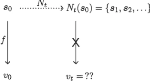
However, also by assumption, the evolution map N is not deterministic, which means that at time t, o could have several possible images {8i, 82,
. . .},
or in other words N(s)could be any non-singleton subset of S. In that case, measurement at time t would not yield a unique answer, with any of the values in {f(si),f(82),.
. .}
being possible.In other words, we have that the determinism of measurement is flot preserved by a non-deterministic dynamics. This situation is depicted in Figure 1.2.
so > N(so) = {si,52,
.
.+
Vtrr??
Figure 1.2: The relationship between states and measurement outcomes in probabilistic models where we have defined a deterministic measurement rule. If the dynamic mapping between states is non-deterministic (represented here by a dotted arrow), then there is not necessarily a unique outeome ut at time t.
Hence, we are ieft with the other scenario in which we no longer have deterministic measurement rules. This important departure from deterministic theories means, among other things, that states no longer determine ail the properties of the system. For ex ample, if the same system eau be “prepared” to be in the same state more than once, the outcome of measurement eau be different each time. Equivalently, two copies of an identical system even if prepared and initialised in the same identical fashion wili yieid different outeome values when observed. However, one thing wiil remain constant for both instances of the system: the relative frequencies of each outcome value. This is how “probabilities” are involved in a probabihstic theory: a system observed under fixed con ditions defines a probabitity distribution or (PD) on the sample space of the measurement variables.
The evolution of a system wili change its characteristies, and in particular these probabibties will change. However, it is expected that these probabilities wili depend on the initial probability distribution, and onty on it. In other words, whiie the measure ments are no longer deterministic, the dynamics between probability distributions of the