CIRPÉE
Centre interuniversitaire sur le risque, les politiques économiques et l’emploi
Cahier de recherche/Working Paper 06-37
Bargaining under Large Risk - An Experimental Analysis -
Werner Güth Sabine Kröger Ernst Maug
Novembre/November 2006
_______________________
Güth: Director Strategic Interaction Group, Max-Planck-Institute for Research into Economic Systems, Kahlaische Strasse, 07745 Jena, Germany. Tel.: +49 (3641) 686 620; Fax: +49 (3641) 686 623
Kröger: CIRPÉE and Economics Department, Laval University, Pavillon J.-A.-DeSève, Québec (QC) Canada G1K 7P4. Tel.: +1 (418) 656 2131 ext. 12896; Fax: +1 (418) 656 2707
Maug: Chair for Corporate Finance, University of Mannheim, 68131 Mannheim, Germany. Tel.: +49 (621) 181 1952; Fax: +49 (621) 181 1980
We thank Tim Grebe for his help conducting the experiment. We are grateful to Charles Bellemare for providing his nonparametric OX-package. We also thank Jan Potters, Karim Sadrieh, Kristian Rydqvist and seminar participants at the Economic Seminar in Stockholm and the ENDEAR workshop in Amsterdam, the ESA International meeting in Boston, SUNY Binghamton and the 4th GEABA-Symposium in Frankfurt a. M. for helpful discussions and for sharing their thoughts on earlier drafts of this paper. Financial support from the Deutsche Forschungsgemeinschaft, SFB 373 and Max Planck Institute for Research into Economic Systems is gratefully acknowledged.
Abstract:
We present an experimental study to learn about behavior in bargaining situations under large risks. In order to implement realistic risks involved in the field, we calibrate the experimental parameters from an environment involving substantial variation in profits, the motion picture industry. The leading example is the production of a movie that may give rise to a sequel, so actors and producers negotiate sequentially. We analyze the data in light of alternative behavioral approaches to understanding bargaining behavior under large risk.
Keywords: Bargaining, Large Risk, Equity, Experiments, Calibration JEL Classification: C72, C91, D81
1 Introduction
The study of ultimatum bargaining in laboratory experiments suggest that individ-uals may be concerned with more than their own profit in evaluating the final out-come of bargaining. Notions of fairness seem to play an important role and equal sharing of the surplus has been shown to be the predominant outcome in many studies investigating behavior in ultimatum bargaining experiments.1
In most of those studies the surplus to share between bargaining parties is cer-tain. This is not very often the case in real life, where various gains from interac-tion might be possible and only their probability rather than the actual realizainterac-tion of the surplus is known to negotiation partners. Sometimes, uncertainty dissolves only after contracts have been specified. Risks involved can be rather substantial and might have an important impact on the behavior of bargaining parties. It is not clear to which extent regularities observed in standard ultimatum bargaining experiments hold under large risk. In this study, we want to shed light on how negotiations develop in the presence of large risks.
In order to study risk of realistic magnitude, we calibrate the experimental pa-rameters based on empirical observations from an environment involving substan-tial variation in profits, the motion picture industry.2 Parameters are determined so as to match the moments of an empirical distribution.3The model developed in this study relates to the structure of the bargaining process in this industry. We present such situations by a two-stage ultimatum bargaining game in which the first period surplus is stochastic. Only in case of a successful outcome at the first stage, i.e., that an agreement is reached and a particular surplus realized, a “sequel project” with a sure outcome can be negotiated with alternation of roles. Such repeated
bargain-1Starting with G ¨uth, Schmittberger Schwarze (1982) there is a large literature on ultimatum
bar-gaining experiments. G ¨uth and Tietz (1990), Roth (1995) and Camerer (2003) provide excellent sur-veys.
2De Vany and Walls (2002) note that “Motion pictures are among the riskiest of products; each
movie is a ‘one-off’ innovation with highly unpredictable revenues and profits.”
3Our calibrations and the data for our study are based on a case study (Teichner and Luehrmann,
1992) that contains data on 99 movies in the 1989-season and some additional data on the profitability of sequels, based on 60 sequels produced between 1970 and 1990. Teichner and Luehrmann base their data on Variety Magazine and some other industry sources.
ing differs from sequential bargaining models in so far, that the second stage is only reached in case of previous agreement, an additional stochastic termination rule and that the surplus is additive.4 The model structure therefore resembles risky partner-ships and cooperations typical also for R&D joint ventures and venture capital.5
Related literature has studied asymmetric information in ultimatum bargaining. Introducing risk or uncertainty about the size of the surplus for the responder has been used to investigate strategic behavior of proposers in ultimatum bargaining games. Results from those studies indicate that notions of fairness appear to re-spond to strategic considerations. Since rere-sponders were deprived of the possibility to compare relative outcomes of proposed allocations and punish selfish offers, pro-posers took advantage of such situation and offered less or demanded more than observed in comparable experiments with symmetric information.6
The main differences of the current study to this literature is that in our study the surplus is extremely stochastic, i.e., involving large stakes and losses, and that there is no private information. Further, we feel that results may not be completely independent of the parameters chosen in the experiment. Choosing parameters that closely resemble those in the field, might illuminate better what happens in risky environments. Surprisingly, calibration of parameters is rarely used in experiments, although we consider it another way to overcome the parallelism problem of the lab and the field.7
4For experimental sequential bargaining studies see Binmore, Shaked, and Sutton (1985), G ¨uth
and Tietz (1990), and Ochs and Roth (1989).
5Venture capital firms finance their portfolio firms in stages. At each stage, the venture capitalist
either negotiates another round of financing or refuses further financing and terminates the relation-ship (Gompers, 1995).
6Results are reported in Mitzkewitz and Nagel (1993), Straub and Murnighan (1995) and Rapoport
and Sundali (1996), who study “offer games” in which the distribution of the stochastic surplus is common knowledge but its realization is private information of the proposer, who offers an amount to the responder. Kagel, Kim and Moser (1996) observe similar strategic behavior of proposers when exchange rates, which are private information and differ between proposer and responder, are re-vealed to the proposer only. Mitzkewitz and Nagel (1993) and Rapoport, Sundali and Seale (1996) study additionally “demand games” in which the distribution of the stochastic surplus is common knowledge but its realization is private information of the proposer, who demands an amount from the (to the responder unknown) realized surplus from the responder.
experi-We can summarize our results as follows. Firstly, responders rarely accept offers below their first-stage opportunity costs. This could be due to the enormous and for experimental studies quite unusual risk subjects face: in our calibrated parametriza-tion the probability of being able to bargain for a lucrative sequel-contract at the second stage is only 25%, so the potential reward is too risky to make subjects pay for this opportunity by foregoing a certain outside option. Thereby proposers either have to become the only risk taker or have no joint project at all. On the other hand, there seems to be little reciprocation by responders who become proposers at the second stage. They hardly offer more than the outside option, keeping 3/4 of the sure second stage surplus for themselves. Interestingly, such self-serving behavior is widely accepted by second stage responders, a result quite different from standard ultimatum bargaining experiments.
We proceed as follows. In section 2, we introduce the model. Section 3 explains the procedure we followed for calibrating the parameters of the model. Details of the experimental design are described in section 4. Section 5 reports general re-sults of the experimentally observed behavior. Section 6 is devoted to developing two behavioral approaches, one based on outcome maximization and an alternative approach based on equity concerns, both of which are confronted with the data in section 7. Section 8 resumes.
2 The Model
We analyze the bargaining between a producer of a movie, denoted by P, and an actor, denoted by A. Movie production is characterized by substantial risks: either the movie is a hit, in which case the producer’s payoff is very large, or the movie is a flop. Then profits are small and often negative. In many cases, producers try to rehire core actors of top-grossing movies to produce a sequel. Producers seem to think that rehiring the main actors of the original is critical to the success of a sequel (in case of “When Harry met Sally,” Meg Ryan and Billy Crystal, in case of
“Rocky,” Sylvester Stallone).8 Clearly, the bargaining power of the actor is high when negotiating the contract for the sequel.9 Core actors of successful films know they are indispensable for the sequel, giving them effective monopoly power.
We present such situations by a two-stage bargaining game where “studios” have ultimatum power when casting the first film. Only if the original film has been successful, actors negotiate a second contract. Actors, now indispensable to the success of a movie the sequel, make a take it or leave it offer to the studio. The game starts with the producer making a wage offer W1 to the actor. If the actor rejects the proposed wage, the game ends with the actor receiving his rather low outside option OA
1 and the producer the profit O1P which could be interpreted as the gain from producing the film with another (presumably less talented) actor.
If the actor accepts the wage offer W1, the movie is produced. Then chance de-termines the success s of the movie, where s ∈ {f , h}. The surplus generated by the movie, to be divided between both bargaining parties, is denoted by C1s. With probability ω the movie is a “hit” (denoted by h) and generates a total surplus C1h, otherwise the movie is a “flop,” denoted by f and generates only C1f < C1h, where 0<ω <1. The profit of the producer is given by Πs1 =Cs1−W1.10
After a “flop” the game ends with the actor earning his wage W1 and the pro-ducer the low profit Π1f of a “flop.” After a “hit” the game proceeds to the second stage. Then the actor proposes a contract for the sequel project. The gain from
pro-8A notable exception are the James Bond-movies that led to a remarkable number of sequels,
albeit with constant blocks of different actors.
9It is common for actors to sign profit sharing contracts. For those contracts, a contrast is often
drawn between actors who have little bargaining power and sign contracts over “net-profit” shares and big stars -such as Tom Hanks- who are able to sign for shares of the “gross-profit” (Weinstein, 1998).
10Note that we do not allow for output-contingent contracts. Chisholm (1997) provides an
em-pirical analysis of profit sharing vs. fixed pay contract choice in the motion picture industry. Her findings suggest that actor share contracts may be offered when the marginal impact of additional effort on the commercial success of the film is expected to be significant. However, we do not model effort-incentives, so the usual reasons for output-related pay do not apply. See Holstr ¨om (1979) and Grossman and Hart (1983) for the traditional argument for output-contingent contracts. See G ¨uth and Maug (2002) for an example of a principal-agent model with effort-incentives where pay is fixed.
ducing the sequel is known to be C2.11 The actor proposes a wage W2that leaves the producer with profits Π2 =C2−W2. The reversal of bargaining power to the agent captures that in case of a “hit” the formerly unknown actor is now a movie star and cannot easily be replaced. Accordingly, his outside option OA
2 could be larger than before what we, however, do not impose since there are no data allowing to estimate the possibly positive difference OA
2 −O1A.
If the producer rejects the actor’s contract offer, the game ends and the actor receives his outside option OA
2 in addition to his previous payoff W1 whereas the producer does not produce the sequel and earns the outside option O2P in addition to his previous earnings Πh
1. If the producer accepts, then both players collect their contractual earnings from both movies. The extensive form of the game is therefore: 1. P offers a wage-contract to A that specifies a fixed wage W1 for A and splits
the uncertain gain from producing the original movie.
2. A can accept or reject. If A rejects, both parties receive their outside payoff and the game ends. If A accepts, the original movie is produced and the game continues.
3. Nature determines the success state s of the movie. Both parties receive a payoff dependent on the success of the movie according to their contract. If the movie is a flop, the game ends. If the movie is a hit, the game continues. 4. A offers P a contract that specifies a fixed wage for A and a fixed profit for P
for producing a sequel to the original movie.
5. P can accept or reject this contract. If P rejects, both parties receive an addi-tional payoff dependent on their outside opportunities and the game ends. If
P accepts, the sequel is produced with gains from production C2that are split according to the contract and the game ends.
11Sequels are a much safer bet. Evidence comes from the case study (Teichner and Luehrmann,
1992) we base our calibration on as well as from Prag and Casavant (1994), who find a positive relation between a film’s revenue and the film being a sequel.
3 Calibrating Parameters
We will determine the parameters of the model so as to match the moments of an empirical distribution. In the following we present the empirical data of movie pro-duction and discuss the calibration. From industry data we determine most param-eters of the model through calibration. The data for calibration are found in the case “Arundel Partners - The Sequel Project” (Teichner and Luehrmann, 1992). The case assembles data for 99 movies produced by 6 major studios released in the United States in 1989. The data in this case study are taken from a database largely based on Variety Magazine, a trade magazine specializing on the movie industry. Based on Exhibit 7 of the case we calculate the net present value (NPV) of a first film as:12
NPV = PV o f Net In f lows at year 1
1.12 −PV o f Negative Cost at year 0. (1) Here, the present value of net inflows are gross box office proceeds in the US, plus international proceeds and revenues from video rentals net of distribution costs and expenses. These are discounted at an estimated cost of capital of 12%. Negative costs include all costs required to make the negative of the film of which prints can be made and rented to theaters. Negative costs include among others the salaries of actors and director, production management, special effects, lighting, and music. Table 1 gives the total number of films per studio, the number of films that generated a positive NPV on the initial investment, and the total net present value over all 99 films for six major Hollywood studios.
Hence, the average value of a first film is $736.6m/99=$7.44m, and 42 films are profitable with the median film making a loss of $2.26m. The standard deviation is $34.16m, showing that movie-production is risky. Also, the risks and payoffs are distributed somewhat unevenly across studios with MCA being by far the most profitable and Sony being the least profitable, making losses on 26 of their 34 films in 1989. The most profitable film in the sample is Batman (Warner Brothers, NPV=
$224.33m), the greatest disaster was The Adventures of Baron Munchhausen (Sony, NPV= −$45.54m).
The case study estimates the value of potential sequels. On average, costs of
Studio Number of films Positive NPV Films Total NPV MCA Universal 14 11 $263.7 Paramount 10 5 $25.7 Sony 34 8 −$55.4 20thCentury Fox 11 5 $23.2 Warner Brothers 19 7 $233.1 Disney 11 6 $246.2 Total 99 42 $736.6
Table 1: Profitability of first films
Parameter Symbol Value Probability of hit ω 0.25 Pie in case of a hit Ch1 68 Pie in case of a flop C1f −10 Pie in case of the sequel C2 33 Outside option actor O1A =O2A 2 Outside option producer OP1 =O2P 7
quels are 120% of the costs of a first film, according to our model largely due to a change in bargaining power resulting in higher wages after a successful first film. Box office proceeds are on average 70% of the first film, and not every successful film in the sense of a large positive NPV leads to a potentially profitable sequel. Hence, on average sequels are less profitable than first (success) films. There are exceptions: Batman 2 was more successful than the original movie! Based on the calibration documented in appendix A we choose the parameters listed in table 2.13 Effectively, we chose the model parameters so as to match the main features of the joint distribution of film values and sequel values (e. g., mean and standard devia-tion, ratio of sequel value to value of first film).
4 Experimental Design and Procedure
Our experimental design exactly matches the sequential game. In order to analyze bargaining behavior we rely on the estimated parameters from the case study. The computerized experiment was conducted at the laboratory of Humboldt University Berlin in November and December 2001. The computer program was developed using the software z-tree (Fischbacher, 1999). 72 Participants –mainly students of business administration, economics and information technology– were recruited via E-mail and telephone. We conducted six sessions, each consisting of two matching groups. To allow for learning, participants interacted for 18 rounds in the two-stage bargaining game. Participants first read the instructions and were then privately informed about their role.14 Roles were neutrally framed as “participant A” and “participant B” for the role of the actor and producer, respectively. In the follow-ing, we continue to refer to participants as “actors” and “producers,” although the experimental subjects were not aware of this interpretation. Participants remained either an actor or producer throughout the whole experiment. One matching group consisted of three negotiation groups each with one actor and one producer. After
13The full calibration results for the parameters are listed in table 9 in appendix A.
every round new actor-producer-pairs were formed randomly.15
Information feedback was as follows: After the first bargaining stage partici-pants were told whether the actor had accepted the producer’s offer. If the offer was accepted, they were informed about the randomly selected pie size and their first stage earnings. After the second stage participants were told whether the producer had accepted the actor’s offer and what they have earned in the second stage. At the end of each interaction participants were additionally informed about their own cumulative payoffs.
A session lasted on average 140 minutes. The exchange rate was DM 2 for one experimental currency unit (ECU).16 Participants were paid their average payoff of all 18 rounds which was on average DM 21. More precisely, producers received on average DM 25 with a minimum payment of DM 1 and a maximum of DM 71. Actors earned on average DM 17 with minimum payments of DM 8 and maximum of DM 26. Additionally, participants were paid an initial endowment of DM 10 and DM 5 for completely answering the post experimental questionnaire.
5 Data: First and Second Stage Offers
At the first stage which involved negotiations about the stochastic joint profit of either−10 (flop) or 68 (hit), we observe in total 648 W1-offers. Table 3 and Figures 1 and 2 report medians, means, and standard deviations as well as histograms of offers, acceptances and rejections on both stages.
At stage one the producer offered on average 0.8 to the actor. In 435 cases actors accepted the offer with a mean of 4.5. Then chance decided for 143 producer-actor-pairs that a “hit” was realized and subjects continued at the second stage. At the second stage parties negotiated about a joint profit of 33. The average amount ac-tors offer to the producer, Π2, is close to the producer’s outside option of 7 with a median Π2-offer of 8 and 47% of all second stage offers were either 7 or 8. Π2
-15Rematching was restricted to matching groups. Participants were not informed about the
restric-tion of rematching within matching groups what should have further discouraged repeated-game effects.
Stage 1 offer (W1)
Nobs Median Mean Std.dev
All 648 3.0 0.8 6.8
Accepted 435 3.0 4.5 4.1 Not accepted 213 −10.0 −6.6 4.8
Stage 2 offer (Π2)
Nobs Median Mean Std.dev
All 143 8.0 8.9 2.9
Accepted 121 8.0 9.3 2.3 Not accepted 22 8.0 6.6 4.4
0 50 100 150 200 250 -10 -5 0 5 10 15 20 25 30 35 rejected accepted
Figure 1: Frequencies and acceptance/rejection of stage 1 o¤ers (N=648).
Figure 2: Frequencies and acceptance/rejection of stage 2 o¤ers (N=143).
15
Figure 1: Frequencies and acceptance/rejection of stage 1 offers (N=648)
Figure 1: Frequencies and acceptance/rejection of stage 1 o¤ers (N=648).
0 10 20 30 40 50 60 70 80 90 100 -10 0 2 4 6 8 10 12 14 16 rejected accepted
Figure 2: Frequencies and acceptance/rejection of stage 2 o¤ers (N=143).
15
Figure 2: Frequencies and acceptance/rejection of stage 2 offers (N=143)
offers below the producer’s outside option are rare (2.1%). Second stage offers with an average offer of 8.9 were mostly accepted (85%), leaving W2 = 24.1 to the ac-tor. The remaining 213 W1-offers with a mean of−6.6 were not accepted and the round finished for these producer-actor-pairs immediately after stage one with both parties receiving their outside option. Furthermore, at stage one negative offers are almost never accepted (2%), and non-negative offers below the outside option are rarely accepted (26%). Offers above the outside option were accepted in 97% of the cases. Figure 3 presents a nonparametric estimate of the acceptance probability as a function of first stage offers. The concave relationship in the range of [−4.5, 2]
of actors. −6 −4 −2 0 2 4 6 8 10 0.2 0.4 0.6 0.8 1.0
First Stage Offer
Acceptance Probability
95% Confidence bounds
Figure 3: Acceptance probability of first stage offers
0 2 4 6 8 10 12 14 16 0.2 0.4 0.6 0.8 1.0
Second Stage Offer
Acceptance Probability
95 % Confidence bounds
Figure 4: Acceptance probability of second stage offers
The nonparametric estimate of the acceptance probability at the second stage is presented in Figure 4. Low dispersion of second stage offers, which additionally were mostly accepted, explain the wide confidence bounds for offers below 7 and almost constantly high acceptance rates around 90% for offers above 8.
After this general description of the results, we will now propose two different behavioral approaches based on profit maximization and equity concerns and
ad-dress the question how well those approaches explain the observed behavior in the experiment.
6 Behavioral Approach
In this section we present two approaches to analyzing the data, one based on the assumption of outcome maximizing decision makers and the other based on equity concerns.
6.1 Outcome maximizing decision makers
Risk-Neutral Agents We first develop behavior in the game by assuming risk
neu-trality of procedures and actors. This solution serves as a benchmark. We solve this game by backward induction. At the second stage, the actor makes a take it or leave it-offer and offers the producer profits according to her outside option. Hence, the wage at the second stage is
W2∗ =C2−O2P , (2)
Π2 =O2P . (3)
At the first stage, the producer makes a take it or leave it offer to A that makes the actor indifferent between accepting and rejecting the offer, so W1∗ +ωW2∗ = O1A. Therefore,
W1∗ =O1A−ωW2∗ , (4)
Π1s =C1s−O1A+ωW2∗ . (5) Equations (2), (3), (4), and (5) together with the assumption that offers (not) worse than the ones derived are (accepted) rejected represent the game-theoretic solution of the game for risk neutral agents.
Relaxing Risk Neutrality: Risk-Averse Actors Now we partially relax the
as-sumption of risk neutrality by assuming that agents are risk-averse. Producers are typically large studios owned by diversified investors. As the risk of movie suc-cess or failure is idiosyncratic, producers can reasonably be assumed to behave as
if they were risk-neutral whereas the same is not true for actors. Moreover, this modelling strategy allows us to build in reservation wages that may vary across ac-tors, and producers may not have full information about actors’ reservation wages in bargaining. Hence, we introduce two assumptions:
• Actors are risk-averse, while producers are risk-neutral. • Producers are uncertain about actors’ risk aversion.
We explore the implications of these assumptions for the game-theoretic solution in turn. Denote the agent’s utility function by U and observe that there is no uncer-tainty at the second stage of the game, hence equations (2) and (4) still represent the solution to the second stage. Then we require:
U(O1A) ≤ ωU(W1+W2∗) + (1−ω)U(W1) (6) for any acceptable W1, where W2∗ is still given from (2). Then, define the lowest
W1that is just acceptable to the agent by bW1. Clearly, for any risk-averse agent bW1 exceeds (4). Also, it follows directly from (6) that any wage offer W1 ≥ O1A will be accepted, even by an infinitely risk-averse agent. Hence, we have:
O1A−ωW2∗ ≤Wb1≤O1A . (7)
In case the agent’s utility function is common knowledge, we would now have
W1∗ =Wb1as before. However, we assume now that bW1is unknown to the producer, who believes that the actor’s reservation wage is drawn from a continuous distri-bution F(Wb1) with density f(Wb1)and support given by (7). Hence, the producer’s expected payoff as a function of her wage offer is:
E(Π(W1)) = h E(C1s) −W1+E(O2P) i F(W1) + (1−F(W1))O2P =hE(C1s+O2P) −W1 i F(W1) + (1−F(W1))O2P (8) where according to our model E¡Cs1¢ = ω·C1h+ (1−ω) ·C1f. Solving first order conditions ∂E(Π(W1))/∂W1=0 yields:17
W1∗+ F(W1∗) f ¡W1∗¢ = E ³ C1s+O2P ´ −OP1 . (9)
17The second order condition for payoff maximization is f0¡W∗
1
¢
We develop a parametric example in appendix B below, which allows us to ob-tain a closed-form solution for (10) and then convert this solution into quantifiable predictions.
Relaxing Risk Neutrality: Risk-Averse Actors and Producers The assumption
that producers are risk-neutral is, given the above mentioned reasons, very likely to hold in reality. Nevertheless, the model will be investigated using a sample of subjects who are randomly assigned to the roles of actors and producers. If we as-sume risk preferences to be equally distributed over both sub-samples, we will also observe risk-averse producers. As we do not pre-select producers in the experiment according to their risk preferences, we relax the assumption of risk neutrality also for producers.
The producer chooses W1in order to maximize
ωF(W1)U(C1h+O2P−W1) − (1−ω)F(W1)U(C1f −W1) + (1−F(W1))U(O2P) (10) A risk-neutral producer would offer at maximum W1 = O1A, what even an in-finitely risk-averse agent would accept. Independent of the risk aversion of the producer, the minimum offer a risk-neutral actor might accept is W1∗(from equation (4)). Therefore, a producer offering W1 < O1A−ωW2∗ could ensure rejection of the contract by the actor. Such offers could come from risk averse producers who are not willing to bear the risk of production. In appendix B we provide the intuition for a risk aversion-threshold parameter.
As we are mainly interested in the case where the movie is produced, we do not explicitly model risk aversion of producers. Relaxing the assumption of risk neutrality for producers allows for self selection of participants either to become a movie producer by offering within the range of equation (7) or to take the outside option by offering a wage
W1 <O1A−ωW2∗. (11)
Hence, all offers below O2Acan be rationalized by game theory introducing also risk aversion for producers. As in reality, we will only observe movies made by risk neu-tral producers (or producers with a sufficient low risk aversion parameter).
Equa-tions (2), (3), and (7) represent the “game-theoretic” prediction (GT) of the game allowing for risk-averse actors, whereas equation (11) captures the self-selection of producers.
6.2 Decision making with Equality Concerns
Our second suggestion to solve the model is based on former results of ultima-tum (bargaining) experiments, according to which one may expect that only claims which aim at equal splits will be accepted.18
Equity theory (Homans, 1961) predicts equal sharing but leaves open what is shared equally.19 This can, for instance, be the total of the expected pie E(C) = E¡C1s+C2 ¢ = h ω(C1h+C2) + (1−ω)C1f i
. Sharing the expected stage pie sepa-rately at each stage would result in W1 = E
¡
C1s¢/2 for the first stage offer and Π2 = C2/2 as second stage offer. However, there exists a range of possible first stage offers within which compensation on the second stage and therefore equal share of the total expected pie is still possible.20 We therefore allow, more generally,
W1 =E(C1s)/2−ω∆ , (12)
Π2 =C2/2−∆ , −C2/2 ≤∆ ≤C2/2. (13) In this respect, equation (13) essentially predicts (positive and negative) reci-procity. Lower offers W1are followed by lower offers Π2such that Π2depends pos-itively on W1.21 Nevertheless, if both agents follow equity considerations, too mea-ger offers, i.e., W1 < E
¡
Cs1¢/2−ωC2/2 and Π2 < C2/2− (1/ω)(E ¡
C1s¢/2−W1), will be rejected. Equations (12) and (13) represent the “equity-theoretic” prediction (ET) of the game.22
18See G ¨uth (1995) and Roth (1995) for surveys.
19See G ¨uth (1988) for an attempt to add specificity to this concept.
20The actor will accept the lower offer and not be compensated with probability(1−ω). If the
producer offers E¡Cs 1
¢
/2−ω∆ at the first stage in case of a hit the actor can offer C2/2−∆. To reach
the equal split he should be compensated by ∆.
21Equity theory would predict Π
2(W1) =C2/2−E
¡
Cs1¢/2ω+W1/ω.
22Other theoretical approaches allowing for other regarding preferences in final outcomes,
con-sider aversion against inequity (Fehr and Schmidt, 1999) or aversion against being above or below the average income of bargaining parties (Bolton and Ockenfels, 2000) or concerns for the least well in the society (Charness and Rabin, 2002).
On the basis of table 2 we can distinguish between the predictions of the two the-oretical approaches: (i) the game-theoretic solution allowing for risk-averse agents (GT) with equations (2)-(5), (7), and (11), (ii) the equity-theoretic solution based on the total expected profit (ET) with equations (12) - (13). Using the experimental parameters above, we obtain the predictions in table 4.
Prediction Acronym Model Predictions
W1 Π2 W2 Game Theory GT [−10, 2.0] 7.0 26.0 GT (i) [−10,−4.5) − − GT (ii) [−4.5, 2.0] 7.0 26.0 Equity Theory ET 4.75−ω∆ 16.5−∆ 16.5+∆ with ∆∈ [−16.5, 26.5]
Table 4: Predictions of game theory allowing for risk averse agents (eqs. (2)-(3), (7), (11))
and equity theory (eqs. (12)-(13))
The game theoretic prediction can be subdivided in: (i) Self-selection of risk-averse producers. and (ii) Allowing for risk-averse actors, assuming risk-neutral producers.
Clearly, given our calibrated parameters game theory and equity theory provide quite different forecasts (see table 4). According to which W1 would lie either in the interval of [−10, 2.0] or[−1.875, 8.875], respectively. Together, both approaches cover 24% of the total action space[−10, 68], which can be decomposed in 15% for GT, 14% for ET, and 5% for an overlapping range at[−1.875, 2].
At the second stage, there is no uncertainty about the joint profit of 33. Following game theory, actors will offer the producer his outside option, Π2 = 7, resulting in a wage–claim (W2) of 26. Whereas according to equity theory, actors would offer Π2 = 16.5, or depending on the deviation from the equal split offer at stage one,
imply that expected profits at each stage are shared equally.23
The implications of the bargaining model differ depending on the theoretical approach applied.
(i) Predictions by game theory depend on the risk preferences of the actor as well
as how desperate the actor is to join the risky project given his outside oppor-tunities.
(ii) Equity theory does not take the outside options of the agents into account and
concentrates only on the expected joint profit.24 It allows for deviations from stage-wise equal split and predicts a certain relation of this deviation.
Hence, game theory requires knowledge of the real outside options of the actor and the producer as well as the risk preferences of the actor.
We will later estimate actors’ risk parameters and producers’ uncertainty about their bargaining partners’ risk preference using the experimental data. From the observed experimental offers we also compute the stage-wise deviation from equal split.
7 Contrasting Behavioral Predictions
The average first stage offer lies in the overlapping range of GT and ET, a fact which seems to support both theories. Nevertheless, only higher offers with an average of W1 = 4.5, ∆ = 1 (see table 3), which fall into the range of the equity prediction (see table 4) were accepted. However, at the second stage, offers are close to the game theoretic solution of 7. How well second stage offers match with the equity prediction can be deduced from the deviation of an equal split of the expected joint profit at stage one. Generally, second stage offers seem to be lower than ET would
23The range of ∆ is determined by the experimental design, i.e., the range in which decision
vari-ables of participants were allowed to lie. Since at the second stage, the highest possible offer could
be C2=33, ∆ could not be lower than−16.5. And since the lowest possible offer was−10, ∆ could
not be greater than 26.5.
24Equity theory does not take outside options into account as long as OA
1 +OP1 ≤E(C)and Oi1≤ E(C/2), for i∈ {A, P}.
predict: given from accepted first stage offers that ∆ = 1, one might expect second stage offers to be around 15.5.
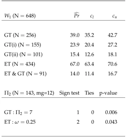
In the following, we investigate the predictive power of the two theories using a nonparametric approach. For stage one, we estimate the probability of the obser-vations to lie within one of the predicted intervals and determine the confidence bounds of these probabilities.25 The probability estimates and their 95% confidence bounds are reported in table 5. The estimates indicate the likelihood that W1 is
of-W1(N=648) cPr cl cu GT (N=256) 39.0 35.2 42.7 GT(i) (N=155) 23.9 20.4 27.2 GT(ii) (N=101) 15.4 12.6 18.1 ET (N=434) 67.0 63.4 70.6 ET & GT (N=91) 14.0 11.4 16.7
Π2(N=143, mg=12) Sign test Ties p-value
GT : Π2 =7 1 0 0.006
ET : ω =0.25 2 0 0.043
Table 5: Probability estimates cPr, 95% confidence bounds (cl and cu), and test statistics of the Sign test (two-sided) based on matching group (mg) averages. (49 W1−offers lie outside
the range of GT and ET.))
fered within the predicted interval of GT to be 39%, whereas with 67% probability the offer lies in the ET interval. The overlapping range of ET and GT comprises 14% of all first stage offers.
25The probability that subject i’s wage offer(W
1,i)lies in the theoretically predicted interval with
the lower bound bland upper bound buis estimated as cPr=cPr(W1,i ∈ [bl, bu]) =1/N ∑iN=11(W1,i∈
[bl, bu])with 1(·)denoting the indicator function. The confidence bounds are estimated as cPr±1.96∗ q
c
Second stage offers are compared to the prediction of GT and ET by a Sign test.26 We test ET by comparing the compensation ratio claimed by second stage offers to its theoretically predicted value. The results of the test reported in table 5 indicate that the GT hypothesis H0 : Π2=7 is rejected in favor for H1 : Π2 6=7,(p=.006).27 Even though second stage offers are close to the GT prediction, they are mainly slightly bigger. According to ET the offer at the second stage will be an equal split of the second stage joint profit adjusted for the deviation of the first stage offer from equal sharing of the expected joint profit. From equation (12) we know that this deviation is: E¡C1s¢/2−W1 =ω∆. The adjustment at the second stage will be equal to the deviation at the second stage weighted by the probability to reach the second stage: C2/2−Π2 = ∆. If behavior is guided by equity principles, then the ratio of stage-wise deviations from equity should be¡E¡C1s¢/2−W1
¢
/(C2/2−Π2) =
ω∆/∆ = ω. Figure 5 plots the density of this “deviation ratio” ( bω) for all second
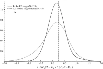
stage offers and additionally in a separate graph of the 123 cases satisfying ET at the first stage. The median of the ratio density is with 21% close to the commonly known probability(ω =25%) of reaching the second stage. The density seems to be skewed to lower ω-values indicating that actors might try to overcompensate “losses” at the first stage in a self-serving way. This overcompensation is significant (p=.043) but the difference of the deviation seems to be small, so that actors do not earn significantly more than producers.28
We can summarize our results so far:
Result 1
(i) Producers frequently offer negative wages W1which are almost never accepted;
W1−offers below the outside option of actors are rarely accepted which can be explained by risk aversion of actors (but not by equity theory). This also
26The Sign test compares the number of positive and negative deviations from the hypothesized
median. For our data the test is appropriate as it does not require symmetry of the data under consideration. The distribution of second stage offers is skewed to the left (see figure 2). To control for individual dependencies, we will report results on the averages of (independent) matching groups.
27This result holds on the individual level at(p=.000).
28In only 3 out of 12 sessions average earnings of actors are higher than average earnings of
−2.0 −1.5 −1.0 −0.5 0.0 0.5 1.0 1.5 2.0 0.2 0.4 0.6 0.8 1.0 _ _ _ ω ( E(C1)/2 − W1 ) / ( C2/2 −Π2 ) In the ET range (N=123)
All second stage offers (N=143)
Figure 5: Density estimate: Ratio of first and second stage deviations according to equity
theory
expresses that producers have to bear the risk of a flop alone or there is no movie production.
(ii) At the first stage equity theory receives generally better support. This suggests
that unequal splits at the first stage are accepted if, in case of a success, the actor is compensated according to forgone profits.
(iii) Equity concerns seem to be indicated less strongly by second stage offers. As
according to equity theory actors (over)compensate at the second stage for first stage inequality by (too) low second stage offers.
(iv) Compared to other ultimatum game experiments, (accepted) second stage
of-fers are very low. Second stage proposals comprise on average 20% of the surplus. Accepted proposals are with an average of 28% of the surplus also surprisingly low.
Together, both theories can explain most observed first stage offers which por-tends that the theories capture different behavioral rules which were applied in the bargaining process. Further analysis of offers which fall in the predicted range of GT (equation (7)) can help to shed light on individual risk aversion of actors and
how producers take the uncertainty of unobserved heterogeneous risk preferences of their bargaining partners into account. Additionally, as both approaches seem to exhibit difficulties explaining behavior at the second stage, individual analysis of the offer and acceptance behavior will expose the applied behavioral rules and whether these can be rationalized in direction of equity or game theory. Therefore, we only summarize results of an analysis and estimation of risk parameters as well as of different individual reactions in stage two which can be found in the Appendix.
7.1 Risk Preferences
Producers Assuming risk-neutral producers and allowing for risk-averse actors,
GT(ii) can account for 15.4% of all first stage offers (see tables 4 and 5). Taking the probability estimate of GT (allowing for risk aversion of all agents) of 39% into account, approximately one-quarter of all first stage disagreements are caused by producers’ risk preferences. In Section 2 (p. 16) we discussed the self-selection op-portunity for producers: offers below W1∗ = −4.5 will never be accepted, a fact which might be used by producers who do not want to get engaged in the risky joint project. In fact, 50% of all producers never offer a wage below this threshold, and 25% of all producers place only one third of their offers below W1∗.
The following analysis of actors’ risk preferences and producers’ uncertainty about their bargaining partner’s risk aversion takes only offers in the interval[−4.5, 2]
(equation (7)) into account, which can be rationalized and have a chance of being ac-cepted according to GT.
Actors First we try to make inferences about actors’ risk aversion from rejected
and accepted offers. Here we assume that actors behave rational over all 18 periods and infer individual risk preferences from their choices. However, for many sub-jects in our experiment the results are not informative,29leaving us with only 15 out of 36 experimental subjects with usable results for estimating risk aversion.
Esti-29In total we excluded 21 subjects from the analysis for one of the following reasons: (1.) subjects
rejected offers of W1 = 2 and higher, which is inconsistent with any interpretation based on
risk-aversion, (2.) the highest offer rejected was smaller than the lower bound W = −4.5, (3.) the lowest
mating risk aversion ρ(Wb1) by the highest rejected offer we obtain individual risk parameters in the range[.69, 7.13].30,31
Uncertainty about risk aversion We model producers’ uncertainty about actors’
risk aversion by choosing a parametric family of probability functions F(Wb) =
³ b
W−W W−W
´γ+1
with W = −4.5 and W =2 in equation (9) above. We apply two ways to estimate the parameter γ. Our first approach is directly using the arithmetic mean of all offers in the range[−4.5, 2]. Our second approach also includes information of answers to those offers and applies maximum likelihood estimation. Details are explained in appendix C. The parameter estimate for γ is γ1 =0.34 for approach 1 and γ2 =2.70 for approach 2. This result suggests that producers seem to underesti-mate actors’ risk aversion when making an offer since γ1lies below γ2, the estimate they would have had they known the answers to their offers, as well as below the range of actors’ estimated individual risk preferences above.32
7.2 Reciprocity
In a second analysis of individual behavior we investigate the repeated response to successful first stage offers. Despite the close resemblance of the data with equity considerations at stage one, actors hardly seem to respond in a way that conforms to the predictions of equity theory at the second stage. Regressing Π2on W1 indicates a constant second stage offer around 9 and no reaction towards the offer at the first
30We estimate risk aversion by stipulating that W
0 =20 (approximately equal to average
experi-mental earnings) and solve equation (19) in appendix B for bW1.
31Another way to estimate risk preferences would be to assume that the acceptance threshold lies
in the middle of the interval of the highest rejected and the lowest accepted offer. For this case, we
can estimate bW1 by averaging the highest rejected and the lowest accepted offer and we obtain a
larger range of risk parameters[.21, 26.17].
32Nevertheless, those findings should be interpreted cautiously as only 44% of the subjects in the
actor position could be used in the estimation of the risk aversion parameter. The decisions of all remaining subjects were not informative because their highest rejected offer did not exceed their
lowest accepted offer. Also the estimation of the γ−parameter of the threshold density function
cannot account for all data. It considers only offers in the interval[−4.5, 2] which comprises only
stage.33 One possible explanation might be that actors react in heterogeneous ways. We will now investigate how individual actors reciprocate. Second stage offers con-ditional on first stage offers indicate three different types of behavior:
• constant offers, i.e., no reaction regardless of the first stage offer,
• reciprocity, reacting to high (low) first stage offers by a increase (decrease) of
second stage offers, and
• idiosyncratic reaction.
We separate those 34 actor-subjects for which the number of second stage expe-riences ranges from 2 to 7 into three subgroups:34
• 6 participants of a constant type (with no variation of Π2) who all offer either
O2P or the equal split (Opportunistic/Fair Proposers),
• 9 reciprocal participants (who respond in kind, i.e., react positively with Π2to
W1) (Reciprocators), and
• 19 participants, who neither relied on the same Π2−offer nor reciprocated (in the above sense) (Experimenters, who try out different offers Π2 in idiosyn-cratic ways).
Four actors of the first type behave rather opportunistically after a hit by of-fering producers essentially their outside option. The remaining 2 actors can be regarded as equity minded with respect to the second stage joint profit with con-stant Π2-offers of 16 and 14. Reciprocators respond to a low (high) wage offer at the first stage by a lowering (increasing) their second stage offer. A linear regres-sion¡Πi2 =α0+α1·W1i+εi
¢
for those participants results in α0 = 6.9 (0.2), α1 = 0.41 (0.04) for the estimates with standard errors in parenthesis and R2 = 0.80.
33Estimation of Π 2on W1 ¡ Πi2=α0+α1·W1i+εi ¢ results in ˆα0=9.3 (0.4), ˆα1= −0.09 (0.07)for
the parameter estimates with standard errors in parentheses and R2=0.01.
34There is a total of 36 actors. Two participants could not be classified. One subject had only once
the chance to make an offer at the second stage. The other person received and offered the same amounts in both cases.
Nevertheless, this reaction is still different from ET, according to which parameter estimates should be close to α0= −2.5 , α1 =4.0. Considering the regression results, a corresponding compensation to a deviation of the first stage offer from equal split seems to be dominated by the presence of the outside option of the producer also for reciprocators.
The idiosyncratic behavior of actors can partly be explained by directional learn-ing. Directional learning (see, for instance, Selten and Buchta, 1998) predicts the direction of changing one’s strategy by adapting it in the direction suggested by an ex-post-analysis of past choices in order to maximize profits. For an actor reaching the second stage directional learning theory would predict that if his offer was re-jected last time it will be increased next time. Similarly, in case of an accepted offer last time one should not increase the offer (or keep it constant). 92% of all idiosyn-cratic offers confirm directional learning.35
Result 2 An analysis of the data at an individual level sheds light on what we can
learn from the different approaches.
(i) Based on first stage offers which fall in the range of the GT, we model proposers’
beliefs about actors’ risk preferences. And based on responses to those of-fers we estimated actors’ actual risk preferences. This analysis indicates that producers overestimate actors’ risk preferences and therefore have to high ex-pectations about the acceptance of low offers.
(ii) There is support for general reciprocation by some second stage offers in the
spirit of ET: 26% of actors reciprocate with their second stage offers and 6% of all actors offered unconditionally the equal split. However, the majority of actors (68%) adjust their offers in a profit maximizing manner.
35The reciprocity analysis should be interpreted cautiously as we observe between 2 and 7 second
stage responses per actor. Nevertheless, it shows, that the current theories are rather questionable in a more complex environment.
8 Summary
This paper has raised the question how bargaining processes evolve over time when large risks are involved. We investigate this question in an explorative experimental way. In order to capture risk involved in the field, we calibrate the experimental parameters using data from a field study on the motion picture industry. In particu-lar, we look at a two period bargaining model, with alternating bargaining position and additive surplus at each stage. In terms of “ movie production,” the negotiation arises between a producer and an actor about how to share the uncertain proceeds from a first movie and in case of a sequel the profits of the second movie with alter-nating bargaining positions.
The model developed here differs from the existing literature in two aspects. First, the surplus at the first stage is stochastic and its realization revealed to both bargaining parties only after establishing a contract. This differs from the existing literature where at least one person is informed about the realization of the stochas-tic surplus. Second, the surplus generated at each stage is additive and the bargain-ing process can only continue if both parties accepted the contract in the previous stage, resembling continuation projects in risky joint ventures.
Our results indicate that despite the riskiness of the business, even in the lab-oratory there is “movie production” as some experimental participants in the role of producers are willing to take on risks. Moreover, according to our data, produc-ers either have to become the only risk taker or there is no movie production at all. We analyze the data in light of two different behavioral approaches, one assum-ing decision makassum-ing is influenced by outcome maximization and individual risk preferences, the other based on the decision makers’ goal to share equally. Look-ing at the data from those two angles, we learn that often production of first films fails since producers underestimate the risk aversion of actors, who seem not to be willing to share the risk with the producer. Interestingly, we observe that at the second stage with the sure surplus, accepted offers are much lower than conven-tional studies on ultimatum bargaining report. This indicates that actors not only offer lower shares to the producer, but also that this behavior is accepted by the pro-ducer. Even though, actors in general behave rather opportunistically, reciprocity
ideas can partly explain other aspects of observed behavior, some actors reciprocate to higher first stage offers by higher second stage offers or share the second stage surplus equally.
Altogether there appears to be some variety in what motivates behavior in such risky bargaining environments, which can neither be captured by assuming pure outcome maximization of decision makers allowing for risk preferences nor by as-suming that their choices are solely motivated by equity theory. It seems that differ-ent motives are competing in such extreme environmdiffer-ents. To which extend fairness considerations survive or are crowded out and what drives the impact of different motives in risky environments remain future research questions.
9 Appendix
A Parameter Calibration
Calibrating Model Parameters. We estimate the profitability of sequels (in present
value terms) estimating NPVs on the basis of projected revenues and costs. Note that the calculations are similar to those above, but for the first films we used ac-tual data, whereas we use projected profitability for sequels based on the stylized facts reported above. Hence, this procedure reflects the expected and not the actual profitability of sequels. For example, it would never predict that a sequel is more profitable than its first film (like Batman 2). Also, while no studio would ever make a sequel with a negative NPV, sequels can turn out to make losses even after a suc-cessful first film. (“Look who is Talking 2” was a disaster.) We can then estimate the value of a sequel right, that is the economic value of the right of the movie studio to produce a sequel after observing the success of the first film. While only a small number of first film gives rise to profitable sequels, the movie studio does not have to produce sequels to flops. Table 6 gives the relevant data.
Studio Profitable Sequels Value of sequel right Sequel/First film
MCA Universal 9 $6.69 30% Paramount 3 $2.68 32% Sony 4 $2.89 35% 20thCentury Fox 2 $1.78 30% Warner Brothers 3 $7.33 42% Disney 5 $10.29 36% Total/Average 26 $4.96 34%
Table 6: Values of Sequels
Hence, based on this model we would project that of 99 films, 26 would generate profitable sequels. Note that even Sony, which had a negative profit for its first films, would have expected positive profits for its sequels, since it would only make sequels of 4 of its 34 films. These data are volatile and can be driven by a small number of outliers. In the case of Sony, a large fraction of projected sequel profits comes from the successful “Look who is talking,” that generates about 80% of its
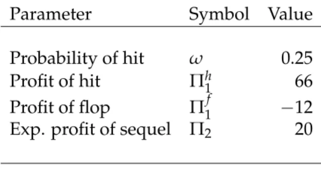
Parameter Symbol Value Probability of hit ω 0.25 Profit of hit Πh1 66 Profit of flop Π1f −12 Exp. profit of sequel Π2 20
Table 7: Parameters
projected sequel profits.36 For our purposes, we now define a “hit” as a film that could give rise to a profitable sequel, hence our hit rate here would be 26/99 or 26.3%. Note that this hit rate probably overestimates the likelihood of a sequel being made, since it includes some movies where the script of the first movie would hardly give rise to a sequel (e.g., “Driving Miss Daisy”).
We reduce the empirical distribution of movies to a binary distribution as fol-lows. A film in our model is either a “hit” and produces a payoff of Πh
1, or a “flop” with a payoff of Π1f, where Πh1 > Π1f. A film is a hit with probability ω, hence the expected profitability of a film is:
µ =ωΠ1h+ (1−ω)Π1f . (14)
The standard deviation of the binary distribution is:
σ=³Π1h−Π1f ´ q
ω(1−ω) . (15)
The value of a sequel after a successful first film is denoted by Π2, hence the value of the sequel right is ωΠ2. We chose the parameters in table 7.
Table 8 compares the actual values in the data, the calibrated values, and the errors between actual and calibrated values. The calibration captures the mean and standard deviation of the data very accurately. The profitability of the sequel and the value of a sequel right is also captured. The typical ratio of the expected profitability of a sequel to a successful first film is 30% for the model values, and 34.1% in the sample.
36Two sequels to this film were made, but their economic success was far lower than expected on
Parameter Symbol Value Data Error Prob. of hit ω 0.25 0.263 −4.8% Expected profit µ $7.50m $7.44m 0.8% Std. dev. σ $33.77m $34.16m −1.1% Exp. prof. of sequel Π2 $20.00m $18.88m −5.6% Sequel/first film Π2/Πh1 30% 34.1% 12.4% Sequel right ωΠ2 $5.00m $4.96m −0.8%
Table 8: Error statistics
Calibrating Sequel Costs. With the calibrated parameters we adjust the values of
the experiment the following way: If the company produces the movie it earns the revenue R and has to bear production costs, consisting of the actor’s wages W and remaining production costs PC. The producer’s profits Π1 in the first stage for the “hit” (Πh
1) and for the “flop” (Π
f
1) as well as profit for a sequel Π2can be written as: Πki =Rik− (Wi+PCi), for i =1, k∈ {f , h}, and i=2 (without k). (16)
For calibrating R2we use the stylized facts as in the case study for the relation of the revenues of a successful film to a sequel, namely
R2 ≈ 107 Rh1. (17)
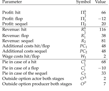
Furthermore, we assume that the additional production costs are the same in the film and its sequel, PC1 = PC2. With this system of equations and the calibrated values of Πh1 =66 (in case of a “hit”), of Π1f = −12 (in case of a “flop”), and Π2 =20 we chose the parameters according to the game with one modification as follows. The field study does not give any evidence for W1 but indicates that the relation of total wage costs to cumulative costs (so called “negative costs” plus distribution expenses) is approximately one to five for a typical film, i.e., 14PC1 > W1. That is why we choose for the calibration of the first stage revenue W1 =O1A=2.
The actor and the producer negotiate about the remaining surplus, Cj = Π1j + O1A = Rj1−PC1, j ∈ {l, h} before the movie is going to be produced. The two possible pie sizes are therefore Ch1 =68 and C1f = −10 for the hit and the flop movie, respectively. In case of a successful first movie the actor and producer negotiate
Parameter Symbol Value Profit: hit Π1h 66 Profit: flop Π1f −12 Profit: sequel Π2 20 Revenue: hit Rh1 116 Revenue: flop R1f 38 Revenue: sequel R2 81
Additional costs hit/flop PC1 48 Additional costs sequel PC2 48
Wage costs hit/flop W1 2
Pie in case of a hit C1h 68 Pie in case of a flop C1f −10 Pie in case of the sequel C2 33 Outside option actor both stages OA 2
Outside option producer both stages OP 7 Table 9: Experimental parameters
about the remaining share of the sequel’s revenue which is C2= R2−PC2 = 107 R1−
PC2 =33, according to equation (17) and the assumption PC1 =PC2.
The outside option for the actor was chosen in order to resemble the outside opportunity for the actor. It additionally separates from offers around “zero” as a natural barrier between positive and negative offers at stage one. At the same time the outside opportunity should not exceed the expected first stage profit nor the equal split prediction described in Section 6. The producer’s outside option should prevent from total bankruptcy but was chosen to be below the expected size of the first stage pie.
As the outside options cannot be deduced from the empirical data, we had to choose them from a reasonable range. To render bargaining at all profitable we had to respect E(Cs
1) >O1A+O1P and C2 >O2A+OP2 where E(·)denotes the expectation operator. In order to keep the whole game simple, both players’ outside options are kept constant at both stages, i.e., OA
1 =O2A =2 and OP1 =OP2 =7. The action space of offers was bound at first stage to the minimum and maximum joint profits, i.e.,
[−10, 68]. At the second stage we kept the lower bound constant and adjusted the upper bound to the joint profit at the second stage, i.e,[−10, 33]. Table 9 displays all
calibrated parameters.
B Parametric Example
Producers Assume producers have outside wealth Π0 and constant relative risk aversion (CRRA) with parameter ρ. Then
U(Π1) = (Π0+Π1) 1−ρ
1−ρ (18)
with Π1 = f (W1). The risk aversion parameter for producers who do not want to get engaged into the risky joint venture at all even when facing a risk neutral agent who would accept W1∗, have a risk aversion parameter ρ such that
U(W1∗) ≤U ³ OP1 ´ ω(Π0+C h 1+OP2 −W1∗)1−ρ 1−ρ − (1−ω) (Π0+C1f −W1∗)1−ρ 1−ρ ≤ (Π0+O1P)1−ρ 1−ρ . Actors Assume actors have outside wealth W0and constant relative risk aver-sion (CRRA) with parameter ρ. Then
U(W1) = (W0+W1) 1−ρ
1−ρ . (19)
This expression can be used directly in (6) and solved for bW1 (at least numerically) in terms of the parameters of the model.
Producers Define the lower and upper bound of the interval (7) by W and W
respectively: W1A−ω ³ C2−OP2 ´ , (20) W1A . (21)
Then choose the following parametric family of distribution functions:
F(W1) = µ W1−W W−W ¶γ+1 with γ∈ [−1, ∞], (22)
which have density
f (W1) = (γ+1) (W1−W)
γ
¡
W−W¢γ+1 (23)
so that the second order condition becomes
γ(W1−W) > 2(γ+1) . (24)
Note that for γ(W1−W) >2(γ+1)this family of distribution functions is suf-ficiently flexible for our example. For γ = −1 we obtain the uniform distribution, for−1 < γ < 0 we obtain distribution functions with the probability mass shifted to the left, and for γ > 0 we obtain distributions with the probability mass shifted to the right. Substituting these into the example above and solving (9) gives:
W1∗ =min ½ W, γ+1 γ+2 ³ E ³ C1s+O2P ´ −OP1 ´ + 1 γ+2W ¾ . (25) We have to guarantee that the solution lies in the interval (7), so the Min-operator makes sure that the expression does not exceed the upper bound W. Hence, for interior solutions W1∗ is a weighted average of the minimum W (the reservation wage for a risk-neutral actor) and the producer’s maximum willingness to pay,
E¡Cs
1+O2P ¢
−OP
1. Paying this amount would reduce the producer’s expected pay-off to his outside option. The solution is intuitive. Observe that
∂W1∗ ∂γ =
E¡C1s+O2P¢−O1P−W
(γ+2)2 >2 (26)
for all solutions. Hence, a distribution that assigns higher probabilities to higher reservation wages also leads to higher equilibrium wage offers. Note also that:
lim γ→∞W ∗ 1 =min n W, E ³ C1s+O2P ´ −OP1 o =W (27) lim γ→−1W ∗ 1 =W (28)
Here, the first result follows from the definition of (20) and (4). Hence, if we choose γ small enough, then the probability distribution degenerates and all prob-ability mass is put on the event where the actor is risk-neutral (W1∗ = W for all γ+1 < 0). Hence, for γ = −1 we recover the original problem and the solution (4), (5). Conversely, for large γ, all actors are deemed to be infinitely risk averse and judge the payoffs from the maximin criterion, so
b W1=O1A Ã W1∗ =W for γ+1> W−W E¡C1s+O2P¢−O1P−W ! .
Equation (25) extends our game theoretic solution to risk averse actors. Its im-portance lies in the fact that we can always find a probability distribution charac-terized by some parameter γ that would rationalize the behavior of producers as an outcome of this game, where producers are uncertain about the actor’s reservation utility. Conversely, offers outside the interval (7) cannot be rationalized at all.
C Modelling Uncertainty about Risk-Aversion
We model the uncertainty about actors’ risk aversion by choosing a parametric fam-ily of probability functions F
³ b
W
´
= ³W−WW−Wb ´γ+1 in (9) in Section 2 (p. 14) above. We apply two ways to estimate γ. Our first approach uses the arithmetic mean of all offers in the range[−4.5, 2]. In appendix B we showed that (9) then becomes:
W1∗ =min ½ W, γ+1 γ+2 ³ E ³ C1s+O2P ´ −OP1 ´ + 1 γ+2W ¾ . (29) We can calculate γ with the offers observed. For this, we insert the experimental parameters and the mean offer in equation (29):
E³C1s+O2P´−OP1 = 17 4 WA1 −ω ³ C2−O2P ´ = −9 2 Then equation (29) reads:
W1∗ =min ½ 2, γ+1 γ+2 µ 17 4 ¶ + 1 γ+2 µ −9 2 ¶¾ . (30)
with γ as the only unknown parameter. The mean (median) offer in the range
[−4.5, 2]is 0.52(0.00)and yields γ=0.34(0.06)from direct substitution into (29). Our second approach to estimate γ is maximum likelihood estimation. We as-sume that the first stage offer W1is accepted (a = 1) when the threshold parameter
b W is reached, i.e., a= 1 if W1≥W,b 0 if W1<W.b hence, the probability of accepting W1is
Pr(a=1) =Pr ³
W1≥Wb ´