Modélisation de l'oscillation Madden-Julian lors de son passage sur l'océan Indien et le continent maritime

(1)

THÈSE

En vue de l’obtention du

DOCTORAT DE L’UNIVERSITÉ DE TOULOUSE

Délivré par : l’Université Toulouse 3 Paul Sabatier (UT3 Paul Sabatier)

Présentée et soutenue le 18/09/2018 par :

Daria Kuznetsova

Modélisation de l’oscillation Madden–Julian

lors de son passage sur l’océan Indien et le continent maritime

(Modelling the Madden–Julian oscillation

during its passage over the Indian Ocean

and the Maritime Continent)

JURY

FRANK ROUX LA, Toulouse Président du Jury

CHRISTELLE BARTHE LACy, La Réunion Rapporteuse SOPHIEBASTIN LATMOS, Guyancourt Rapporteuse

PETER HAYNES DAMPT, Cambridge Rapporteur

DOMINIQUE BOUNIOL CNRM, Toulouse Examinatrice

JEAN-PIERRE CHABOUREAU LA, Toulouse Directeur de thèse

École doctorale et spécialité :

SDU2E : Océan, Atmosphère, Climat Unité de Recherche :

Laboratoire d’Aérologie, Université de Toulouse, CNRS, UPS Directeur de Thèse :

Jean-Pierre Chaboureau Rapporteurs :

(2)

(3)

Modelling the Madden–Julian

oscillation

during its passage over the Indian

Ocean and the Maritime Continent

Author:

Daria K

UZNETSOVA

Supervisor:

(4)

(5)

Preface

Going abroad for studies was a big step for me and I want to thank all people who made it possible. I am very grateful to everyone in Laboratoire d’Aérologie (LA)/ Observatoire Midi-Pyrénées/ Université Paul Sabatier (UPS) for welcom-ing me in Toulouse.

Thanks to the French Ministry of Higher Education and Research (Ministère de l’Enseignement supérieur et de la Recherche) for providing me a Ph.D. student scholarship.

Thanks to the LA directors Céline Mari and Frank Roux and to the Doctoral School “Sciences de l’Univers, de l’Espace et de l’Environnement” (SDU2E) direc-tors Geneviève Soucail and Patrick Mascart, as well as to the assistant director Stéphane Bonnet.

Thanks to my advisor Jean-Pierre Chaboureau (LA) for introducing me to the subject of meteorology that I had previously known nothing about, and for giving me an opportunity to learn a lot.

Thanks to my thesis defense committee members: Frank Roux (LA), Chris-telle Barthe (LACy, La Réunion), Sophie Bastin (LATMOS, Guyancourt), Peter Haynes (DAMPT, Cambridge), Dominique Bouniol (CNRM, Toulouse). Their valuable remarks and comments helped to improve this manuscript.

Thanks to Chantal Claud (LMD, Paris) and Dominique Bouniol for being in my thesis evaluation committee during these three years, their feedback was of a great help for me.

Thanks to many others for reviewing and discussing my work, especially to Frank Roux, Eric Defer, Evelyne Richard. Also, thanks to the students, postdocs and interns, especially to Thibaut Dauhut and Irene Reinares Martínez for their

(6)

explanations and assistance, as well as to Laurent Labbouz, Nicolas Blanchard, Keun-Ok Lee, Léo Seyfried, Flore Tocquer, Phillip Scheffknecht and many others.

Thanks to the IT support team for their assistance.

Thanks to all the administrative support staff for their help in arranging the paperwork, especially to Karine Mercadier (LA), Marie-Claude Cathala (SDU2E), and Catherine Stasiulis (UPS).

Many thanks to Marisa Vialet (LA) for her constant encouragement, help and advices.

Also, special thanks go to Olga Krivonosova and Dmitriy Zhilenko from the Institute of Mechanics of Moscow State University, and to Maria Gritsevich from the University of Helsinki, for their support and discussions.

Getting to love science in all its forms is a life journey. I want to thank with all my heart my family, friends, and generally — every person who inspired me, helped me and motivated me on this journey, be it many years ago or during these three years of my Ph.D. studies.

I would like to finish this preface with beautiful words spoken by the person whose passion for science and whose views of the world have inspired so many people.

Carl Sagan, “Pale Blue Dot,” 1994 – about an image of the Earth taken by Voyager 1 spacecraft on 14 February, 1990.

Look again at that dot. That’s here. That’s home. That’s us. On it everyone you love, everyone you know, everyone you ever heard of, every human being who ever was, lived out their lives. The aggregate of our joy and suffering, thousands of confident religions, ideologies, and economic doctrines, every hunter and forager, every hero and coward, every creator and destroyer of civilization, every king and peasant, every young couple in love, every mother and father, hopeful child, inventor

(7)

and explorer, every teacher of morals, every corrupt politician, every “superstar,” every “supreme leader,” every saint and sinner in the history of our species lived there — on a mote of dust suspended in a sunbeam.

The Earth is a very small stage in a vast cosmic arena. Think of the rivers of blood spilled by all those generals and emperors so that, in glory and triumph, they could become the momentary masters of a fraction of a dot. Think of the endless cruelties visited by the inhabitants of one corner of this pixel on the scarcely distin-guishable inhabitants of some other corner, how frequent their misunderstandings, how eager they are to kill one another, how fervent their hatreds.

Our posturings, our imagined self-importance, the delusion that we have some privileged position in the Universe, are challenged by this point of pale light. Our planet is a lonely speck in the great enveloping cosmic dark. In our obscurity, in all this vastness, there is no hint that help will come from elsewhere to save us from ourselves.

The Earth is the only world known so far to harbor life. There is nowhere else, at least in the near future, to which our species could migrate. Visit, yes. Settle, not yet. Like it or not, for the moment the Earth is where we make our stand.

It has been said that astronomy is a humbling and character-building experience. There is perhaps no better demonstration of the folly of human conceits than this distant image of our tiny world. To me, it underscores our responsibility to deal more kindly with one another, and to preserve and cherish the pale blue dot, the only home we’ve ever known.

(8)

(9)

Abstract

The Madden–Julian Oscillation (MJO) is the dominant component of the in-traseasonal variability in the tropical atmosphere, propagating eastward in the equatorial band. It consists of a convective center (active phase) accompanied by the low-level zonal wind anomaly convergence and the upper-level zonal wind anomaly divergence, and zones of weak convection (suppressed phases). Three time periods of the MJO activity over the Indian Ocean and the Maritime Conti-nent were chosen: 6–14 April 2009, 23–30 November 2011, and 9–28 February 2013. The simulations with and without convective parameterizations were per-formed for a large domain with the atmospheric model Méso-NH. It was obtained that the simulations with parameterized convection were not able to reproduce an MJO signal. For 2009 and 2011 when the coupling between convection and large-scale circulation was strong, the convection-permitting simulations showed a visible MJO propagation, which was not the case for 2013. For the 2011 episode, the processes contributing to the suppression of the convection were studied using an isentropic analysis to separate the ascending air masses with high equivalent potential temperature from the subsiding air masses with low equivalent potential temperature. Three large-scale circulations were found: a tropospheric circulation, an overshoot circulation within the tropical tropopause layer, and a circulation of air masses with low equivalent potential temperature in the lower troposphere. The latter corresponds to the large-scale dry air intru-sions from the subtropical zones into the equatorial band, mostly found during the suppressed MJO phase over the Indian Ocean.

(10)

Résumé

L’oscillation de Madden–Julian (MJO) est la composante dominante de la variabilité intrasaisonnière dans l’atmosphère tropicale, se propageant vers l’est dans la bande équatoriale. Elle se compose d’un centre convectif (phase active) accompagné de la convergence des anomalies du vent zonal de bas niveau et de la divergence de niveau supérieur, et de zones de convection faible (phases supprimées). Trois périodes de l’activité MJO sur l’océan Indien et le continent maritime ont été choisies : 6–14 avril 2009, 23–30 novembre 2011 et 9–28 février 2013. Les simulations avec et sans paramétrisation de la convection ont été réalisées pour un grand domaine avec le modèle atmosphérique Méso-NH. Il a été obtenu que les simulations avec convection paramétrée n’étaient pas ca-pables de reproduire un signal MJO. Pour 2009 et 2011, lorsque le couplage entre la convection et la circulation de grande échelle était fort, les simulations avec convection explicite ont montré une propagation visible de la MJO, ce qui n’a pas été le cas pour 2013. Pour 2011, les processus contribuant à la sup-pression de la convection ont été étudiés avec une analyse isentropique pour séparer les masses d’air ascendantes ayant une température potentielle équiv-alente élevée des masses d’air subsidentes ayant une température potentielle équivalente faible. Trois circulations de grande échelle ont été trouvées : une circulation troposphérique, une circulation de percées nuageuses dans la couche de tropopause tropicale, et une circulation de masses d’air à faible température potentielle équivalente dans la basse troposphère. Cette dernière correspond aux intrusions d’air sec de grande échelle des zones subtropicales dans la bande équatoriale, trouvées principalement pendant la phase supprimée de la MJO sur l’océan Indien.

(11)

Introduction

A remarkable characteristic of the tropical convection and circulation is their possibility to organize into large-scale patterns. The most important such pattern in the tropical atmosphere is the Madden–Julian Oscillation (MJO), a planetary-scale phenomenon with the zonal extent of the order of 10000 km. The MJO is represented by the coupled signals in atmospheric circulation and deep con-vection, which move eastward over the Indian and Pacific Oceans having a lo-cal intraseasonal period of 30-90 days. It can be distinguished in particular as an eastward-propagating spatial configuration consisting of intensified and sup-pressed precipitation, accompanied by a coherent signature in cloudiness, lower-and upper-level wind, lower-and many other fields such as the sea surface temperature and the evaporation at the surface of the ocean (Madden and Julian, 1971, 1972; Zhang, 2005).

The MJO is the dominant component of the intraseasonal variability in the tropical atmosphere. It interacts with convection on different scales, giving a broad influence on different local and global weather and climate phenomena such as rainfall patterns (Donald et al., 2006), active and break monsoon cycles (Goswami, 2005; Pai et al., 2011), tropical cyclone activity (Liebmann et al., 1994; Klotzbach, 2014; Duvel, 2015), El Niño–Southern Oscillation (ENSO) (Moore and Kleeman, 1999; Kapur et al., 2012) and so on. The influence of the

(14)

MJO extends to higher latitudes through teleconnections creating such phenom-ena as flooding, wildfires, lightning, cold air outbreaks and heat waves, strato-spheric water vapor and aerosols transport, as described in the review of Zhang (2013). Thus, the MJO might influence the occurrence of extreme precipita-tion events in North America (Higgins et al., 2000), can modulate the Arctic sea ice (Henderson et al., 2014), interact with the Arctic Oscillation (Zhou and Miller, 2005; L’Heureux and Higgins, 2008) and North Atlantic Oscillation (Cas-sou, 2008), influence the Antarctic circumpolar transport and the atmospheric Southern Annular Mode (Matthews and Meredith, 2004). Given such a broad influence of the MJO on the weather and climate, studying its fundamental prop-erties is therefore crucial for our understanding of the physics of the tropical atmosphere.

Different theories link the MJO initiation and propagation with such pro-cesses as convective heating, surface evaporation, interactions with the midlat-itudes, boundary layer moisture convergence, Kelvin or Rossby waves (Wang, 2005; Zhang, 2005). At the same time, there is no agreement in explaining the MJO properties e.g. its period/frequency or propagation speed, as well as in defining the driving processes of the MJO. The MJO has been a subject of numer-ous studies, programs, and campaigns that were dedicated to the exploration of the MJO characteristics and the improvement of the MJO simulations and predic-tions. For example, the MJO Working Group (MJOWG) was established by the US Climate Variability and Predictability Program (CLIVAR) and was active in 2006–2009. Its activity continued further in 2010–2013 by forming of the MJO Task Force (TF) which was included into the Year of Tropical Convection (YOTC) program. The diagnostics (“set of metrics”) were developed for assessing the model performance in the MJO simulations (CLIVAR Madden–Julian Oscillation Working Group: Waliser et al., 2009). A number of large field campaigns

(15)

dedi-cated to the MJO took place with the objective to gather in-situ atmospheric and oceanic data over the equatorial Indian and western Pacific Ocean, such as TOGA COARE (Tropical Ocean and Global Atmosphere Coupled Ocean–Atmosphere Re-sponse Experiment) in 1992–1993 (e.g. Webster and Lukas, 1992; Godfrey et al., 1998), MISMO (Mirai Indian Ocean Cruise for the Study of the MJO Onset) in 2006 (e.g. Yoneyama et al., 2008), CINDY/DYNAMO/AMIE (Cooperative Indian Ocean Experiment on Intraseasonal Variability/Dynamics of the Madden–Julian Oscillation/Atmospheric Radiation Measurement Program MJO Investigation Ex-periment) (e.g. Yoneyama et al., 2013; Zhang et al., 2013; Zhang and Yoneyama, 2017) in 2011–2012. This resulted in the creation of an extensive database, nev-ertheless, many questions still remain unresolved.

The numerical simulations of the MJO still are not always able to reproduce a visible MJO signal. Global climate models with the coarse horizontal grid spac-ing have difficulties in reproducspac-ing a realistic signal of the MJO, sometimes they can not even reproduce its eastward propagation (Slingo et al., 1996). One of the reasons is the parameterization of the convection in such models. Thus, the subgrid-scale processes associated with convection are approximated resulting in large biases. In contrast, the convection-permitting models with the horizon-tal resolution ∼1 km allow the convection to be resolved, and the topographic features are more precisely described. This gives these models a potential for the improvement of the MJO simulation and thus, a possibility for the better comprehension of this phenomenon.

The objective of this thesis is to describe the evolution of the atmosphere and the changes in the convective activity during the passage of the MJO, and to demonstrate the processes that are contributing to its propagation. Several simulations are performed by means of the atmospheric model Méso-NH (Lafore et al., 1998; Lac et al., 2018) over a large domain covering the Indian Ocean and

(16)

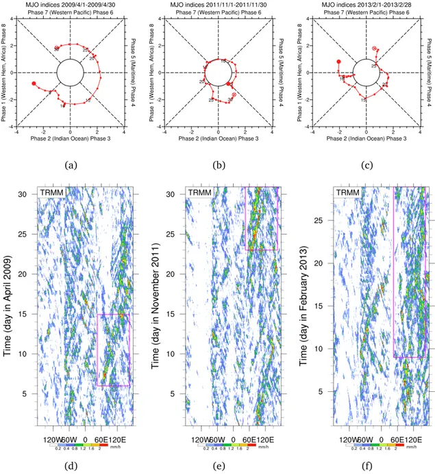
the Maritime Continent. To find out how the resolution and the representation of convection influences the MJO simulation, the model is run at low resolution where convection is parameterized, and at high resolution where convection is explicit. Three MJO episodes are considered: (1) 6–14 April 2009, (2) 23– 30 November 2011, and (3) 9–28 February 2013. These cases correspond to the periods when the MJO was active over the Indian Ocean and the Maritime Continent, where the MJO is generally the most visible. The evaluation of the simulations is performed using a satellite precipitation product and the ECMWF analyses.

The manuscript is organized into the four major sections. In chapter 1, a general overview of the MJO is given. The notions necessary to understand the context of this thesis are introduced, and the ways to identify the MJO signal in observations or simulations are presented. The existing hypotheses concerning the processes contributing to the MJO evolution are explained, and the repre-sentation of the MJO in the numerical models is discussed.

In chapter 2, the cases of study are presented. The non-hydrostatic mesoscale atmospheric model Méso-NH is described with the configurations necessary for the performing of the simulations. Two different types of simulations are pre-sented: the low-resolution simulations with the parameterized convection and the high-resolution convection-permitting simulations. The datasets used for the evaluation of the simulations are described.

Chapter 3 presents the evaluation of the simulations. The results of the simulations with the parameterized convection are compared with those of the convection-permitting simulations as well as with the “reference” datasets. The sensitivity of the convection-permitting simulation to the turbulence scheme and the subgrid-scale cloud fraction parameterization is examined for the episode of 23–30 November 2011.

(17)

The dry air intrusions during the MJO propagation are discussed in chap-ter 4. The isentropic method used in this study is presented. Its principles are discussed, and it is explained how the atmospheric circulations of air masses can be described in terms of the isentropic diagrams. The application for the analy-sis of the evolution of the atmospheric circulations that exist during the passage of the MJO is shown. The results are presented in the article The three

atmo-spheric circulations over the Indian Ocean and the Maritime Continent and their modulation by the passage of the MJO under review in Journal of the Atmospheric Sciences.

Finally, the conclusions are given, and some perspectives for future work are proposed.

(18)

(19)

Introduction (en français)

Une caractéristique remarquable de la convection et de la circulation dans les tropiques est leur possibilité de s’organiser en structures de grande échelle. La structure la plus importante dans l’atmosphère tropicale est l’oscillation de Madden–Julian (MJO) qui est un phénomène à l’échelle planétaire avec une étendue zonale de l’ordre de 10000 km. La MJO est représentée par des sig-naux couplés dans la circulation atmosphérique et la convection profonde, qui se déplacent vers l’est au-dessus des océans Indien et Pacifique avec une période intrasaisonnière locale de 30 à 90 jours. En particulier, elle peut être décrite comme une alternance entre des zones de précipitations inténsifiées et de pré-cipitations réduites, accompagnée d’une signature cohérente dans les nuages, les vents troposphériques dans les basses et les hautes couches et de nombreux autres champs comme la température de surface de la mer et l’évaporation à la surface de l’océan (Madden and Julian, 1971, 1972; Zhang, 2005).

La MJO est la composante dominante de la variabilité intrasaisonnière dans l’atmosphère tropicale. Elle interagit avec la convection à différentes échelles, donnant une large influence sur différents phénomènes météorologiques et cli-matiques locaux et globaux tels que les précipitations (Donald et al., 2006), les moussons (Goswami, 2005; Pai et al., 2011), la cyclogenèse (Liebmann et al., 1994; Klotzbach, 2014; Duvel, 2015), la El Niño–Southern Oscillation (ENSO)

(20)

(Moore and Kleeman, 1999; Kapur et al., 2012) etc. L’influence de la MJO s’étend à des latitudes plus hautes par le biais des téléconnexions qui créent des phénomènes tels que les inondations, les feux de forêts, les éclairs, les vagues de froid et de chaleur, le transport de vapeur d’eau et d’aérosols dans la stratosphére, comme décrit dans la revue de Zhang (2013). Par conséquent, la MJO pourrait influencer l’occurrence des précipitations extrêmes en Amérique du Nord (Higgins et al., 2000), moduler la banquise arctique (Henderson et al., 2014), interagir avec l’oscillation arctique (Zhou and Miller, 2005; L’Heureux and Higgins, 2008) et l’oscillation nord-atlantique (Cassou, 2008), influencer le transport circumpolaire antarctique et le mode annulaire austral (Matthews and Meredith, 2004). Puisque la MJO a une influence importante sur la météorologie et le climat, l’étude de ses propriétés fondamentales est donc cruciale pour notre compréhension de la physique de l’atmosphère.

Différentes théories relient l’initiation et la propagation de MJO à des pro-cessus tels que le chauffage par convection, l’évaporation de surface, les inter-actions avec les latitudes moyennes, la convergence de l’humidité de la couche limite, les ondes de Kelvin ou de Rossby (Wang, 2005; Zhang, 2005). En même temps, il n’y a pas d’accord pour expliquer les propriétés de la MJO, par ex. sa période / fréquence ou vitesse de propagation, ni pour définir les processus de pilotage de la MJO. La MJO a fait l’objet de nombreuses études, programmes et campagnes consacrés à l’exploration de ses caractéristiques et à l’amélioration de ses simulations et de sa prévision. Par exemple, le Groupe de travail sur la MJO (MJO Working Group, MJOWG) a été créé par le Programme américain de variabilité et de prévisibilité du climat (Climate Variability and Predictability, CLIVAR) et a été actif en 2006–2009. Son activité s’est poursuivie en 2010–2013 avec la création de la Task Force MJO (TF) qui a été incluse dans le programme YOTC (Year of Tropical Convection). Les diagnostics ont été développés pour

(21)

évaluer la performance des modèles dans les simulations de la MJO (Waliser et al., 2009)). Des grandes campagnes de terrain dédiées à la MJO ont eu lieu dans le but de recueillir des données atmosphériques et océaniques in situ sur les régions équatoriales de l’océan Indien et Pacifique Ouest, telles que TOGA COARE (Tropical Ocean and Global Atmosphere Coupled Ocean–Atmosphere Re-sponse Experiment) en 1992–1993 (e.g. Webster and Lukas, 1992; Godfrey et al., 1998), MISMO (Mirai Indian Ocean Cruise for the Study of the MJO Onset) en 2006 (e.g. Yoneyama et al., 2008), CINDY/DYNAMO/AMIE (Cooperative Indian Ocean Experiment on Intraseasonal Variability/Dynamics of the Madden–Julian Oscillation/Atmospheric Radiation Measurement Program MJO Investigation Ex-periment) (e.g. Yoneyama et al., 2013; Zhang et al., 2013; Zhang and Yoneyama, 2017) en 2011–2012. Cela a permis de créer une base de données étendue, mais de nombreuses questions restent toujours sans réponses.

Les simulations numériques de la MJO ne sont pas toujours capables de re-produire un signal MJO visible. Les modèles climatiques globaux avec un es-pacement grossier de la grille horizontale ont des difficultés à reproduire un signal réaliste de la MJO, parfois ils ne peuvent même pas reproduire sa prop-agation vers l’est (Slingo et al., 1996). L’une des raisons est la paramétrisation de la convection dans de tels modèles, ainsi les processus d’échelle sous-maille associés à la convection sont approchés, ce qui conduit à des biais importants. En revanche, les modèles permettant la convection avec une résolution horizon-tale ∼1 km permettent de résoudre la convection et de décrire plus précisément les caractéristiques topographiques. Cela donne à ces modèles le potentiel de mieux simulare la MJO et donc la possibilité d’une meilleure compréhension de ce phénomène.

L’objectif de cette thèse est de décrire l’évolution de l’atmosphère et les changements dans l’activité convective lors du passage du MJO et de montrer les

(22)

processus qui contribuent à sa propagation. Pour ce faire, plusieurs simulations sont effectuées à l’aide du modèle atmosphérique Méso-NH (Lafore et al., 1998; Lac et al., 2018) sur un vaste domaine couvrant l’océan Indien et le continent maritime. Pour déterminer comment la résolution influence la représentation de la MJO, le modèle est lancé à basse résolution où la convection est paramétrée, et à haute résolution où la convection est explicitement représentée. Trois épisodes MJO sont examinés: (1) du 6 au 14 avril 2009, (2) du 23 au 30 novembre 2011 et (3) du 9 au 28 février 2013. Ces cas correspondent aux périodes pendant lesquelles la MJO était active sur l’océan Indien et le continent maritime, où la MJO est généralement la plus visible. L’évaluation des simulations est réalisée à l’aide du produit de précipitation satellitaire et des analyses ECMWF.

Le manuscrit est organisé en quatre sections principales. Dans le chapitre 1, un aperçu général de la MJO est donné. Les notions nécessaires à la com-préhension du contexte de cette thèse sont présentées et les moyens d’identifier le signal MJO dans les observations ou les simulations sont présentés. Les hy-pothèses existantes concernant les processus contribuant à l’évolution de la MJO sont expliquées et la représentation de la MJO dans les modèles numériques est discutée.

Dans le chapitre 2, les cas d’étude sont présentés. Le modèle méso-échelle atmosphérique non-hydrostatique Méso-NH est décrit avec les configurations

nécessaires pour l’exécution des simulations. Deux types différents de

sim-ulations sont présentés : les simsim-ulations à basse résolution avec convection paramétrée et les simulations à haute résolution avec convection résolue. Les jeux de données utilisés pour l’évaluation des simulations sont également décrits. Le chapitre 3 présente l’évaluation des simulations. Les résultats des simula-tions avec convection paramétrée sont comparés avec ceux des simulasimula-tions avec convection résolue ainsi qu’avec les ensembles de données de référence. La

(23)

sen-sibilité de la simulation avec convection résolue au schéma de turbulence et à la paramétrisation de la fraction nuageuse d’échelle sous-maille est examinée pour l’épisode du 23 au 30 novembre 2011.

Les intrusions d’air sec pendant la propagation de la MJO est étudié dans le chapitre 4. La méthode isentropique qui est utilisée pour cette étude est présentée. Ses principes sont discutés et il est montré comment les circulations atmosphériques des masses d’air peuvent être décrites par les diagrammes isen-tropiques. Les résultats sont présentés dans l’article The three atmospheric

circu-lations over the Indian Ocean and the Maritime Continent and their modulation by the passage of the MJO en révision dans Journal of the Atmospheric Sciences.

Enfin, les conclusions sont données et des perspectives de travail futur sont proposées.

(24)

(25)

Chapter 1 The Madden–Julian oscillation

1.1 Overview of the MJO

1.1.1 Definition

The MJO, Madden–Julian Oscillation, became known to the scientific commu-nity from the work of Madden and Julian in 1970s (Madden and Julian, 1971, 1972), though as noted by Li et al. (2018), it was documented in an earlier study of (Xie et al., 1963) in a Chinese journal. The MJO is an eastward-moving large-scale phenomenon (zonal extent around 12000–20000 km) and the dom-inant component of the intraseasonal variability in the tropical atmosphere. It is represented by coupled patterns in atmospheric circulation and convection and accompanied by a coherent signal in many other variables (Zhang, 2005). Thus, the MJO propagation can be traced in precipitation, zonal wind, Outgoing Longwave Radiation (OLR), humidity, water vapor etc.

The MJO consists of a zone of strong precipitation and deep convection, i.e.

active phase, which is flanked to the east and to the west by zones of weak

precipitation and convection, i.e. suppressed phases. The schematic structure

of the MJO is depicted in Fig. 1.1 where the cloud symbol shows the convective center and the arrows show the direction of zonal wind anomalies. West of the convective center, low-level westerlies and upper-level easterlies are present while to the east of the convective center, low-level easterlies and upper-level westerlies are present, thus giving a convergence of the zonal wind close to the surface and a divergence in the upper troposphere.

(27)

Figure 1.1: Schematic representation of the MJO structure. The cloud symbol shows the con-vective center. The shaded zones indicate the negative OLR anomalies. The horizontal arrows represent zonal wind anomalies at 850 and 200 hPa and the vertical arrows represent the ver-tical velocity anomalies at 500 hPa. Letters “A” and “C” indicate the anticyclonic and cyclonic circulation centers, respectively. Reproduced from Rui and Wang (1990).

Figure 1.2: Schematic representation of the MJO structure showing the position of the convective center relative to the low-level wind convergence/upper-level wind divergence structure. Arrows width denotes their amplitudes. Curves at the bottom represent intraseasonal perturbations in sea surface temperature induced by the MJO, positive anomalies are located above the horizontal lines. Reproduced from Zhang (2005).

convergence/upper-level wind divergence structure is not constant. Four differ-ent configurations are shown in Fig. 1.2. During the MJO propagation over the

(28)

Indian Ocean, the convective center is generally located between the low-level westerlies to the west and easterlies to the east, shown as Model I in Fig. 1.2. Over the Pacific Ocean, the convective center is generally located to the west of the low-level wind convergence, shown as Model II in Fig. 1.2. Model III in Fig. 1.2 is theoretically predicted and Model IV is obtained in some numerical simulations, but neither of these configurations was observed (Zhang, 2005).

The MJO propagates eastward around the globe (Fig. 1.3), however, its speed and amplitude vary during its propagation as well as among different MJO events. The convective activity is generally the strongest over the Indian and western Pacific Oceans where the sea surface temperature (SST) is the highest,

with an average speed of the MJO being 5–10 m s−1_{, while over the eastern}

Pacific convection is much weaker and the MJO is mostly marked by the wind

anomalies and larger speed of 10–15 m s−1_{. The Indo–Pacific Maritime}

Conti-nent is known for its “barrier effect” on the MJO, as the MJO often weakens or completely disappears during its passage over this region (e.g. Rui and Wang, 1990; Zhang and Ling, 2017). Nevertheless, in some cases the MJO initiates outside the Indian Ocean (Mattews, 2008; Bellenger and Duvel, 2012).

The MJO is a multi-scale phenomenon. Its active phase consists of a number of small-scale convective systems moving in different directions, e.g. Nakazawa (1988) notes the successive formation of convective cloud clusters inside the MJO (Fig. 1.4). In particular, while the MJO moves eastward as a whole, inside its active phase it is possible to see small-scale cloud clusters moving westward.

The satellite images of MJO signature in the water vapor channel in the equatorial band over the Indian Ocean are shown in Fig. 1.5 for 0000 UTC and 1200 UTC 23 November 2011, and 0000 UTC and 1200 UTC 24 Novem-ber 2011. The development of the MJO and the eastward propagation of the large-scale envelope can be easily observed. The active MJO phase can be seen

(29)

Figure 1.3: Schematic dia-gram showing the propaga-tion of the MJO. The cloud symbol represents the con-vective center of the MJO. The line at the top indicates the tropopause height. In the bottom of the charts, the mean pressure disturbance is shown, negative anoma-lies being shaded. The ar-rows show the associated zonal circulation. Time in-creases from top to bottom, from “F” to “H” and then from “A” to “E”. This diagram was constructed by Madden and Julian (1972) based on their observations at Can-ton Island (3◦_S,172◦_{W), “A”} corresponds to the moment when the minimum pressure wave was observed. Repro-duced from Madden and Ju-lian (1972).

(30)

Figure 1.4: Schematic diagram showing the formation of cloud clusters inside the MJO. To the left, the existence of multiple eastward-moving super clusters during the active MJO phase is shown. To the right, the super cluster structure is represented. Reproduced from Nakazawa (1988).

as the large area of high water vapor content and deep convective clouds (white colour) while the suppressed MJO phase corresponds to a dry zone following the active phase.

The intraseasonal period of the MJO is 30–90 days (Madden and Julian, 1972; Zhang, 2005) though the MJO is not a regular periodic oscillation, its strength and period vary from one event to another. Due to the non-regular character of the MJO, Mattews (2008) stated that it is better to use the term “MJ event” rather than “MJO”, describing the MJO as a series of discrete events rather than an oscillation. The irregularity of the MJO is also seen in the atmo-spheric conditions between two consecutive events: an MJO event can develop

after a quiet period (primary MJ events, according to Mattews (2008)) as well

as redevelop from a previous cycle (successive MJ events in Mattews (2008)).

Thus, the search of the MJO precursors in the atmosphere and the description of the initiation of the MJO are not well defined problems.

(31)

(a) (b)

(c) (d)

Figure 1.5: Meteosat satellite images showing the propagation of an MJO episode in 2011 as seen in water vapor over the Indian Ocean: (a) 0000 UTC 23 November, (b) 1200 UTC 23 November, (c) 0000 UTC 24 November, (d) 1200 UTC 24 November. Approximate wavelength range 5.7– 7.1 µm, Mid-IR / Water vapor. The white colour shows the high content of water vapor and deep convective clouds and corresponds to the active MJO phase. Behind the areas with large water vapor content, areas with low water vapor content are seen, which shows the suppressed MJO phase located behind the active phase. The images are reproduced from the Web site of the NERC Satellite Receiving Station, Dundee University, Scotland: http://www.sat.dundee.ac.uk/.

(32)

1.1.2 Identification

The propagation of the MJO signal in the atmosphere can be described by choosing a method that shows (i) the presence of the MJO event, as indicated by a defined threshold, and (ii) the location of the active MJO phase in the tropical band.

Straub (2013) categorizes these methods in three groups based on:

• cloudiness: typically Outgoing Longwave Radiation (OLR), precipitation (e.g. Rui and Wang, 1990; Hendon and Salby, 1994; Hendon et al., 1999; Matthews and Kiladis, 1999; Kemball-Cook and Weare, 2001; Myers and Waliser, 2003; Benedict and Randall, 2007; Ling et al., 2014; Kerns and Chen, 2016);

• atmospheric dynamics (circulation): zonal wind velocity, velocity poten-tial (e.g. Krishnamurti and Subrahmanyam, 1982; Lorenc, 1984; Knutson et al., 1986; Knutson and Weickmann, 1987; Poehl and Matthews, 2007; Chen and Del Genio, 2009; Tromeur and Rossow, 2010);

• combined cloudiness and circulation (e.g. Weare, 2003; Wheeler and Hendon, 2004).

Methods using the principal component analysis. A classical method is

based on the principal component (PC) analysis. It shows that it is possible to isolate the signal of the MJO in minimally filtered daily data by projection onto spatial patterns characteristic of the MJO. In this method, the empirical orthog-onal functions (EOFs) are calculated based on daily data (e.g. wind, OLR, . . . ) available for a long enough time period, i.e. over several decades. The data are usually averaged over the range of latitudes corresponding to the equatorial band and filtered to remove the large-scale (seasonal, interannual and decadal)

(33)

Figure 1.6: Spatial structures of EOF1 and EOF2 of the combined analysis applied to OLR, zonal wind speed at 850 hPa, and zonal wind speed at 200 hPa (each field is normalized by its global (all longitudes) variance before the EOF analysis). —, OLR; – –, zonal wind speed at 850 hPa; -- --, zonal wind speed at 200 hPa. Reproduced from Wheeler and Hendon (2004).

variability. Generally, two first EOFs are sufficient to represent the MJO signal. Then, a phase diagram is constructed where the axes are the corresponding PCs: PC1 and PC2. A typical MJO event is thus represented as a loop in the phase space. A so-called “index” is obtained where each point denotes the amplitude of PC1 and PC2 at a given time, and a specific direction of rotation corresponds to the eastward MJO propagation. The resulting diagram is divided into parts corresponding to different regions of the tropical band: (i) Indian Ocean, (ii) Maritime Continent, (iii) Western Pacific, (iv) Western Hemisphere and Africa.

(34)

Thus, the location of a point on this curve traces the location of the MJO active phase in the tropical band. The distance between the origin (PC1=0, PC2=0) and a point of the curve shows the amplitude of an MJO event. Usually, a circle with a radius equal to a particular critical value is chosen to distinguish between the non-MJO periods and the MJO activity periods. This representation of the MJO is used in a large number of studies (e.g. Lorenc, 1984; Knutson and We-ickmann, 1987; Lo and Hendon, 2000; Mattews, 2008).

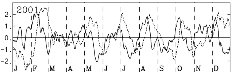
One MJO index well known in the literature, is the RMM index described

in the work of Wheeler and Hendon (2004), where RMM stands for “Real-Time Multivariate MJO series”. The EOFs are calculated for combined OLR and zonal wind speed at 850 hPa and 200 hPa (Fig. 1.6). Each field is normalized by its global (all longitudes) variance before the EOF analysis. Multiplication of each normalized field and the global variance gives the corresponding anomaly that occurs for 1 standard deviation perturbation of the PC, as given for the corre-sponding absolute maxima of this field. Physically, EOF1 corresponds to the enhanced convection (negative OLR anomalies) at the Maritime Continent, low-level westerly wind anomalies over the Indian Ocean and Maritime Continent, and low-level easterly wind anomalies over the Pacific Ocean, while upper-level wind anomalies are in the opposite direction to those of the low-level. EOF2 cor-responds to the enhanced convection over the Pacific Ocean and wind structure in close quadrature to that of EOF1.

The RMM1 and RMM2 (Fig. 1.7) correspond to the normalized PC1 and PC2. The variations representing the MJO are visible, with noise existing during the absence of the MJO. The RMM2 is lagging RMM1 by 10–15 days.

The RMM index (Fig. 1.8) is constructed in a diagram with the axes

(RMM1, RMM2). Thus, the RMM index is a combined cloudiness- and

(35)

am-plitude is considered as strong (thus showing the period of MJO activity) if it is greater than 1, which is one standard-deviation anomaly in the RMM index. There are also other indices which are either cloudiness-based (Mattews, 2008; Kiladis et al., 2014) or circulation-based (Ventrice et al., 2013).

Figure 1.7: The RMM1 and RMM2 time series for 2001. Adapted from Wheeler and Hendon (2004).

Figure 1.8: (RMM1, RMM2) diagram for the periods of December–January–February in 1974– 2003. “Phases” from 1 to 8 are defined as in Wheeler and Hendon (2004) for the easier iden-tification of the MJO location in the tropical band. Phases 2 and 3 correspond to the Indian Ocean, phases 4 and 5 — to the Maritime Continent, phases 6 and 7 — to the Western Pacific, and phases 8 and 1 — to the Western Hemisphere and Africa. Reproduced from Wheeler and Hendon (2004).

(36)

1.2 Processes governing the evolution of the MJO

There exist different hypotheses that try to describe the MJO properties such as its period, propagation speed, or multi-scale structure (e.g. the reviews of Zhang (2005); Wang (2005)). Nevertheless, the mechanisms governing the propagation of the MJO are still a matter of discussion among different stud-ies. It must be also outlined that the MJO is not a solution of the classical Mat-suno (1966) analysis which identifies distinct propagating modes as westward mixed-Rossby-gravity and equatorial Rossby waves, and eastward Kelvin waves. One way to explain the existence of the MJO is to consider it as a response of the atmosphere to an independent forcing mechanism. Such mechanisms can be stationary or moving heating source in the tropics (Hu and Randall, 1994, 1995; Salby and Garcia, 1987; Yu and Neelin, 1994) or extratropical perturbations (Hsu et al., 1990; Lau et al., 1994; Matthews et al., 1996; Lin et al., 2000).

Another way is to describe the MJO as an instability arising from the inter-action between large-scale dynamics and the convective heating. The major hy-potheses to explain this instability consider the interaction of convective heating and large-scale wave motion (wave-CISK, Conditional Instability of the Second Kind) (Lau and Peng, 1987); the “evaporation-wind feedback” (EWF) (Neelin et al., 1987) or “wind-enduced surface heat exchange” (WISHE) (Emanuel, 1987; Yano and Emanuel, 1991); or the friction-induced moisture-convergence interaction (Wang, 1988).

Other important processes are the role of water vapor accumulation (Bladé and Hartmann, 1993), the convective-radiation feedback (Hu and Randall, 1994, 1995), the influence of the seasonal mean circulation and moist static energy distribution (Wang and Xie, 1997) or the thermodynamic feedback between

(37)

at-mosphere and ocean (Flatau et al., 1997; Wang and Xie, 1998; Waliser et al., 1999).

It was found in the observations (Myers and Waliser, 2003; Johnson and Ciesielski, 2013; Xu and Rutledge, 2014) that the free-tropospheric moisture profile is influenced by the MJO passage, thus modifying the large-scale orga-nized convection. Several MJO models were constructed based on the coupling of the convection and the moisture, suggesting that the MJO can be explained as a moisture mode instability (Raymond and Fuchs, 2009; Sobel and Maloney, 2013; Adames and Kim, 2016).

The difficulty to explain the MJO properties arises from the fact that all the processes mentioned above contribute to it. Different theories can be interrelated and it is too complicated to analyze a particular process without making several approximations and thus probably neglecting other processes.

The interaction between the large-scale dynamics and convection is more and more often considered to be essential for the MJO. Before the active MJO phase, the free troposphere is humidified, which is also associated with the development of clouds and facilitates convection. Deep convection heats the troposphere and leads to a large-scale dynamic response, which creates the westerly (easterly) wind anomalies to the west (east) of the convective center in the lower tropo-sphere. The westerly wind over the Indian Ocean intensifies and increases the ocean–atmosphere fluxes, which influences the development of deep convection by providing humid air into the lower layers of the troposphere. Hence, the large-scale circulation favours rising motion and contributes to the further de-velopment of convection.

The explanation of the MJO period and the eastward propagation is also complicated (Zhang, 2005; Risi and Duvel, 2014). A hypothesis to explain the period of the MJO is the mechanism of moisture recharge-discharge. During the

(38)

suppressed MJO phase, the atmosphere is dry. The oceanic mixing layer, the sea surface, and the atmospheric boundary layer are gradually warming up due to the effect of strong solar radiation and weak turbulent fluxes of evaporation (latent heat) and energy (sensible heat) in weak wind conditions. The energy and moisture of the atmospheric boundary layer increase, then convective clouds start to develop and to humidify the low troposphere. After the developing of cumulus congestus clouds (up to around 5 km), the moisture is transported up-wards and thus humidify the middle troposphere. This humidification seems to be essential for triggering deep convection. In fact, convective plumes can be weakened by the entrainment of cooler and drier surrounding air. In the pres-ence of strong humidity, convective plumes will be more developed and reach higher altitudes (up to 15 km) giving more precipitation. The evaporation of the precipitation would then be weaker, which limits the cooling of the lower layers and thus, the stabilization of the atmosphere. The typical MJO period of 30–60 days could therefore be representative of the time needed to humidify the whole troposphere and to create favourable conditions for very deep con-vection. The accumulated convective energy will then be dissipated by the deep convective clouds associated with the active phase of the MJO. In this recharge-discharge mechanism, the initiation of the active phase can be determined by different factors, like perturbations from mid-latitudes or the MJO propagation itself, e.g. the return of the MJO signal to the western Indian Ocean after it has completed a tour of the Earth could initiate a new MJO event and thus influence its periodicity (Mattews, 2008).

The eastward propagation is a characteristic of Kelvin equatorial waves, thus these waves were naturally considered as an explanation for the MJO propaga-tion. Equatorial wave theory, however, does not provide a simple explanation of the observed frequency and velocity of the MJO. The speed of Kelvin waves is

(39)

about three times faster than the speed of the MJO. Attempts have been made to explain this difference (e.g. Lau and Peng, 1987; Wang, 1988), but the results have not shown a correct MJO-like phenomenon. Some processes for the expla-nation of the eastward speed of the MJO are related to thermodynamics e.g. the cooling of the surface to the west of the convective center, while the eastern re-gions are kept convectively unstable. Other processes are related to the dynamic characteristics such as the meridional circulations that develop on both sides of the equator west of the convective region and contribute to the stabilization of the atmosphere by carrying dry air from the mid-latitudes.

The fundamental processes relevant to the MJO are shown in Fig. 1.9. The marble shading represents the convective relationships with dynamics that are considered to be essential for the understanding of the MJO: the interactions of convective heating, low-frequency equatorial waves (Rossby and Kelvin), bound-ary layer processes, and moisture distribution. Also, other processes are shown: impact of seasonal mean flows, air–ocean interaction and cloud–radiation feed-back. The background circulations could explain the seasonal behaviour of the MJO.

1.3 Observations and simulations of the MJO

1.3.1 Field programs dedicated to the MJO

Due to the importance of the MJO in weather and climate, several campaigns and projects had been carried out to gather in-situ observations. This is essential to be able to test the hypotheses on the MJO-related processes, validate the numerical models, and further improve them.

(40)

Figure 1.9: Fundamental processes relevant to the MJO. Reproduced from Wang (2005).

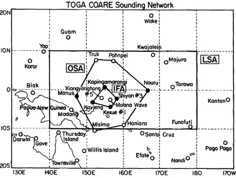
TOGA COARE campaign. Tropical Ocean and Global Atmosphere Cou-pled Ocean–Atmosphere Response Experiment (TOGA COARE) was held dur-ing November 1992 – February 1993 to observe the properties of the MJO in the western Pacific warm pool (Fig. 1.10). Such processes were observed as the ocean-atmosphere interaction, westerly wind bursts, precipitation, surface fluxes, equatorial waves (Godfrey et al., 1998). The objectives were to study the organization of the convection, the ocean–atmosphere coupling processes, the oceanic response to combined buoyancy and wind-stress forcing, and the scale interactions contributing to the influence of the western Pacific warm-pool system to other regions and vice versa (Webster and Lukas, 1992). Three MJO episodes occurred during this campaign as seen in the westerly wind bursts,

(41)

preceded by the heavy precipitation 1–3 weeks earlier. The maximum wester-lies were generally located between two synoptic-scale cyclonic gyres, often not symmetric with respect to the equator in the low-level wind field. In four cases, tropical cyclones developed from the gyres. Important MJO characteristics were observed such as the strong low-level convergence and upper-level divergence as well as the multi-scale structure with the signals in atmospheric variables and SST organized on lengthscales 10–10000 km and timescales from hours to weeks (Webster and Lukas, 1992; Chen et al., 1996).

Figure 1.10: TOGA COARE sounding network, consisting of nested arrays: large-scale array (LSA), outer sounding array (OSA), intensive flux array (IFA). Integrated sounding systems (ISS) are indicated by the solid circles, other sounding stations, by the open circles. Reproduced from Lin and Johnson (1996).

MISMO campaign. The Mirai Indian Ocean Cruise for the Study of the MJO

Onset (MISMO) was dedicated to the study of the MJO convection onset mecha-nism in the equatorial Indian Ocean and conducted in October–December 2006 by the Japan Agency for Marine–Earth Science and Technology (JAMSTEC). The

(42)

observations were made with the research vessel (R/V) Mirai, moored buoys, and several land-based sites at the Maldive Islands (Fig. 1.11).

Figure 1.11: Observation network of MISMO campaign. Atmospheric sounding array is shown in red, dashed. Oceanic buoy array is shown in blue, dashed. Stationary observation site (0◦_, 80.5◦_{E) of the R/V Mirai is represented by the solid diamond. Cruise tracks of the R/V Mirai} (leg 1 and leg 2) are shown in black solid and dashed lines. Reproduced from Yoneyama et al. (2008).

This campaign focused on the air-sea interaction, variations of the ocean surface, evolution of the low-tropospheric moisture convergence and vertical profiles of cloud-related atmospheric parameters and of the wind (Yoneyama et al., 2008). Among other results, the evolution of the convective activity was observed: suppressed in late October – early November, developing in mid-November, and strong activity over the Indian Ocean in late November preceded by gradual deepening of the convection in the divergence field. The precondi-tioning of the development of the active MJO phase is suggested to be related to the easterly propagating cloud systems which contributed to the deepening of the moist layer and are being driven, in particular, by shallow convection (Katsumata et al., 2009). Also, the appearance of large-scale cloud systems was accompanied by the abrupt change in the upper-tropospheric zonal wind from

(43)

westerlies to easterlies, which was probably related to equatorial Rossby waves.

CINDY/DYNAMO/AMIE campaign. The most extensive international field

campaign dedicated to the MJO, Cooperative Indian Ocean Experiment on In-traseasonal Variability (CINDY)/ Dynamics of the Madden–Julian Oscillation (DYNAMO)/ Atmospheric Radiation Measurement Program (ARM) MJO Inves-tigation Experiment (AMIE) (Yoneyama et al., 2013; Zhang et al., 2013; Zhang and Yoneyama, 2017), took place in 2011–2012.

Figure 1.12: DYNAMO/CINDY/AMIE sounding network. The high-frequency soundings (yellow and red dots) and priority sounding sites (black dots) are shown, as well as the research vessels Sagar Kanya (S. K.) and Baruna Jaya (B. J.), which were active for brief periods (25 Sep–19 October for S. K. and 5–18 December for B. J.). Reproduced from Johnson and Ciesielski (2013).

It was focused on tropical intraseasonal variability and in particular, on the MJO life cycle. The CINDY/DYNAMO/AMIE campaign consisted of a sounding-radar array that was formed by a number of research vessels as well as island sites, aircrafts, and enhanced moorings inside and near the array (Fig. 1.12). Its objective was to gather in-situ atmospheric as well as oceanic data over the equatorial Indian Ocean, e.g. related to the structure of cloud and precipitation, moistening, heating, surface fluxes, mixing, and turbulence (https://www.eol. ucar.edu/field_projects/dynamo).

(44)

MJO events that occurred during the October–November 2011, is shown. The signals in the zonal wind, moisture, vertical wind, temperature are distinct. Also, the observational data (middle) show the signals in SST, which is decreasing dur-ing the active phase, while Tropical Rainfall Measurdur-ing Mission (TRMM) satellite data shows the rainfall increase during the MJO passages. The active MJO phase is thus forming after the gradual moistening of the low and middle troposphere (Johnson and Ciesielski, 2013). The relative humidity and wind structure al-low for the developing of cumulus, congestus, and finally, deep convection. In the upper troposphere and lower stratosphere, tilted warm/cool temperature anomalies and zonal wind anomalies are visible, demonstrating the initiation of gravity or Kelvin waves by the MJO (Kiladis et al., 2001; Virts and Wallace, 2010; Virts et al., 2010).

1.3.2 Representation of the MJO in the numerical models

The numerical simulations and predictions of the MJO remain a big chal-lenge as the models struggle to represent the MJO realistically. Often, the models can not reproduce a coherent propagation of the MJO envelope from the Indian Ocean into the Pacific Ocean. Other typical problems are e.g. too weak ampli-tude or too short period, incorrect spatial and temporal distributions, incorrect eastward propagation speed.

In global circulation models (GCMs) with the horizontal grid spacing of the order of 100 km, the realistic representation of the MJO depends on the convec-tion parameterizaconvec-tion as well as on many other factors such as model physics or mean background state. Among the common difficulties are the reproducing of the propagation of the MJO as shown in multi-model studies (Slingo et al., 1996; Lin et al., 2006; Kim et al., 2011), the interaction between the MJO and

(45)

Figure 1.13: Top: Schematic representation of vertical structure of two MJOs during the period 1 October–15 December 2011 (based on average fields measured by the northern sounding ar-ray). Green (yellow) color shows areas with the relative humidity greater than 70% (less than 40%), respectively. Thin black arrows indicate the locations of zonal wind maxima. Thick gray arrows represent the locations of the vertical motion maxima. The dashed line shows the daily averaged 0◦_{C level. The solid line denotes the cold-point tropopause level. The indications “cool”} and “warm” correspond to the centers of cool and warm temperature anomalies. Middle: Hourly SST at the R/V Revelle. Bottom: The daily-averaged rainfall rate over the northern sounding array, according to TRMM 3B42. Reproduced from Johnson and Ciesielski (2013).

the rainfall diurnal cycle (Peatman et al., 2015), the transition from shallow to deep convection that takes place prior to the development of the active MJO phase (Del Genio et al., 2012).

A possible approach to improve the parameterizations is tuning them e.g. to modify the relationship between the convection and the environmental moisture (Zhang and Mu, 2005; Bechtold et al., 2008) or to include convective momentum transport (Wu et al., 2007; Ling et al., 2009). Also, in regional models with parameterized convection the nudging of a certain field from the global analyses

(46)

can be performed e.g. for moisture (Hagos et al., 2011; Subramanian and Zhang, 2014). These approaches can be helpful but their disadvantage is the lack of proper physical justification of the relationship between the MJO convection and the changed field, thus other aspects of the simulations can be degraded.

Including the air-sea coupling might be helpful (Shinoda and Hendon, 1998; Waliser et al., 1999; Maloney and Sobel, 2004; Woolnough et al., 2007) but this interaction is not always necessary for the MJO simulation as some atmospheric models could simulate the MJO without the coupling with the ocean (Hendon, 2000).

Another approach is to use the superparameterizations where instead of the convection parameterization, 2D cloud-system-resolving models are used in each grid cell of the global model and they interact through the large-scale dynam-ics. Mesoscale convection is explicit in these models and the parameterization is done not for cumulus but for the cloud microphysics. Such models allow to bet-ter simulate the MJO or MJO-like systems (Liu et al., 2009; Benedict and Ran-dall, 2009; Grabowski, 2003; Khairoutdinov et al., 2005). Nevertheless, these simulations are computationally expensive and another drawback is that the 3D structure of convection can be important for the MJO simulations.

There have been attempts to simulate the MJO with single-column models, where the forcing data can be taken from observations (Abdel-Lathif et al., 2018), GSM simulations (Woolnough et al., 2010), or even high-resolution convection-permitting simulations (Christensen et al., 2018). However, the chal-lenge here is to derive the required forcing data, and the final analysis might be impacted by different factors such as the missing data, insufficient temporal res-olution, etc.

Finally, the models with the resolved subgrid scale processes are very promis-ing. The increase of the resolution allows these models to reproduce mesoscale

(47)

features that were not resolved previously by a convective parameterization. This gives a more accurate description of the physics of convective systems in numerical weather prediction (Done et al., 2004). Despite the need of “spinup” time when the high-resolution model progressively develops structure from the analysis with lower resolution, there can be a significant improvement in the reproducing of the precipitation (Lean et al., 2008). Convection-permitting sim-ulations allow also to develop and improve parameterizations in the models with parameterized convection, e.g. by studying the moist thermodynamic processes that determine the time scale and energy of the MJO (Hagos and Leung, 2011). Comparing the simulations performed by the same model but with explicit and parameterized convection can be especially beneficial to see the impact of the explicit treatment of convection (Holloway et al., 2013, 2015). Convection-permitting models with a realistic MJO signal show that the relationship be-tween the moisture and the convection is a key process for MJO initiation and propagation (Holloway et al., 2013, 2015; Takemi, 2015).

In this work, we use the atmospheric non-hydrostatic regional model Méso-NH (Lafore et al., 1998; Lac et al., 2018) which allows us to perform low-resolution simulations with parameterized convection and high-low-resolution simu-lations with explicit convection. There have been very few cases of the MJO sim-ulations run with Méso-NH. It was used as a single-column model with the forc-ing data taken from a GSM for model intercomparison (Woolnough et al., 2010) of three periods during the TOGA–COARE campaign. It has been found that dur-ing the transition from the suppressed phase to the active phase, Méso-NH usdur-ing its available convection parameterization is unable to capture the moistening, drying out and giving lower precipitation rates than most of the other models. In the Ph.D. work of Meetoo (2014) dedicated to the study of tropical cycloge-nesis in the Southwestern Indian Ocean, the active MJO phase was detected in

(48)

the Méso-NH simulations of the cyclone Alenga in November–December 2011. A sequence of nested domains was used with the horizontal resolutions of 32 km, 8 km and several domains with the resolution of 2 km following the cyclone trajectory.

Apart from that, there have been no detailed investigation of the capacity of the Méso-NH model to reproduce the MJO signal and especially using the explicit representation of convection. Thus, one of the objectives of this thesis is to evaluate the capacity of Méso-NH to simulate the MJO and to examine the impact of using explicit convection in a very large domain, which nowadays became possible thanks to the improved performance of parallel computing. Another objective is to study the evolution of the atmosphere during the MJO passage and the processes accompanying the propagation of MJO.

(49)

Chapter 2 Model, data and methods

2.1 The Méso-NH model

2.1.1 General description

The Méso-NH (Lafore et al., 1998; Lac et al., 2018) is an atmospheric non-hydrostatic regional model developed by the Laboratoire d’Aérologie and Cen-tre National de Recherches Météorologiques (CNRM) since 1993 (model–related documents can be found on the Web site: http://mesonh.aero.obs-mip.fr/). The Méso-NH model makes it possible to perform simulations with a different resolution, from large synoptic scales (order of 100 km and more, e.g. depres-sions, anticyclones) to convective scales (order of 100 m, e.g. small vortices in the surface boundary layer) to turbulent scales, thus allowing for modeling a large variety of the atmospheric phenomena.

In Méso-NH, the anelastic approach is used which allows to eliminate the acoustic waves from the considered set of equations. In the continuity equation and in the momentum equation the fluid density is approximated by the constant density profile except in the buoyancy term. The anelastic approximation uses the assumption that the atmosphere will stay close to a chosen “reference state”, which is considered here to correspond to the horizontally averaged initial pro-files over the simulation domain.

The prognostic variables are the wind velocity components (u, v, w), the po-tential temperature (θ), the subgrid scale turbulence kinetic energy (TKE), the mixing ratio of water vapor and hydrometeors i.e. solid and liquid precipitating and nonprecipitating water particles (the mixing ratio is the ratio of the mass of considered substance to the mass of dry air within the considered volume). Up to seven different mixing ratios can be chosen depending on the cloud

mi-crophysics scheme: vapor (rv), cloud droplets (rc), rain water (rr), cloud ice

(51)

us-ing a diagnostic pressure equation that is based on the motion and continuity equations.

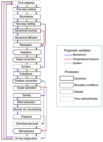
The Méso-NH code consists of three steps: (i) the preparation step of a sim-ulation where the initial fields are chosen; (ii) the temporal integration, starting with the initialization step (Fig. 2.1); (iii) the post-processing step where addi-tional diagnostic fields are computed.

Figure 2.1: Block diagram representing one integration time step in Méso-NH. Reproduced from Lac et al. (2018).

(52)

2.1.2 Dynamics

Theadvection schemes in Méso-NH are of two kinds: those for momentum

and those for scalar variables. The available advection schemes for momentum are flux-form conservative schemes centered in time. The available advection schemes for scalar variables are positive definite schemes. In this work, for the wind advection a 3-order scheme of WENO (Weighted Essentially Non Oscilla-tory) type is used, and for the advection of thermodynamic variables, the PPM (Piecewise Parabolic Method) scheme is used.

Méso-NH uses aC-grid in the Arakawa convention (Mesinger and Arakawa,

1976), both on the horizontal and on the vertical (Fig. 2.2). The meteorologi-cal variables (temperature, water substances, TKE) and the smeteorologi-calar variables are calculated in the center of grid cells (the mass points) while the momentum components are calculated on the faces of grid cells (the flux points). Heat ex-changes, water phase transitions, subgrid scale processes or surface interactions are not taken into account in the dynamical core of Méso-NH and need to be parameterized.

2.1.3 Physical parameterizations

The surface schemes are externalized in the SURFEX (Surface Externalisée)

model (Masson et al., 2013) (http://www.cnrm-game-meteo.fr/surfex/) cou-pled with Méso-NH. The surface and the atmosphere interact via energy fluxes applied at the base of the atmospheric numerical model. The fluxes provided to the atmospheric model are the momentum flux, turbulent sensible and la-tent heat fluxes, the upward radiative fluxes, and, as an option, the CO2 flux.

(53)

5 1 2 3 4 6 7

Figure 2.2: C-grid in the Arakawa convention. 1 — mass points, 2 — u points, 3 — v points, 4 — w points, 5 — vertical vorticity point, 6 — vorticity components along y, 7 — vorticity components along z.

The fraction of the grid cell corresponding to each surface type, is calculated, and then for every type the corresponding surface flux describing the surface-atmosphere interactions, can be computed. The main processes of SURFEX are schematically represented in Fig. 2.3.

For the four main surface types — sea, nature, town, and inland water — the following surface schemes are used. For natural soils, Méso-NH uses the Interac-tions between Soil, Biosphere, and Atmosphere (ISBA) parameterization (Noil-han and Planton, 1989). The input data for the ISBA scheme are the horizontal wind speed, humidity, pressure, temperature of air, precipitation, radiation, and concentrations of dust if necessary. The hydrology is represented by three soil layers where the evolution of water content is calculated by ISBA from the evap-oration and precipitation. Over the urban (artificial) areas, the Town Energy Budget (TEB) is used (Masson, 2000). Lake surfaces are described by the fresh-water lake model (FLake) (Mironov et al., 2010). Ocean surfaces in SURFEX are characterized by the sea surface temperature (SST) and the ocean surface currents. In Méso-NH, it is possible either to use the fields prescribed from the observations or analyses, or use the coupling with an oceanic model such as

(54)

de-Figure 2.3: The main processes of SURFEX depending on the surface type: sea, nature, town, inland water. Reproduced from Masson et al. (2013).

scribed in Gaspar et al. (1990); Voldoire et al. (2017). For the exchanges over sea surfaces, the surface fluxes are parameterized for a wide range of wind and environmental conditions (Belamari and Pirani, 2007). In this work, the SST is constant in time and is provided by the ECMWF analyses at the initial time.

To parameterize the energy transfers from unresolved to resolved scales, a

turbulence scheme is used. In Méso-NH, the turbulence is described by the

1.5-order closure scheme of Cuxart et al. (2000), where the TKE is prognostic and the mixing length is diagnostic. This scheme can be set in 1D mode as well as in 3D mode. In the 1D mode, the subgrid scale interactions between the grid cells are supposed to be only vertical while the horizontal fluxes are neglected, thus using the hypothesis of the horizontal homogeneity. This corresponds to the thermal turbulence which is mostly vertical. This method uses the mixing length

(55)

of Bougeault and Lacarrère (1989) and is usually activated in the mesoscale simulations. In the 3D mode, the dynamic turbulence is considered leading to the transports in all directions. The subgrid scale parameters in a grid cell thus depend on those in all the neighbour cells. This method uses the 3D mixing length of Deardorff (1980) and is usually activated in the large-eddy simulations (LES). Nevertheless, the use of 3D mode in a mesoscale simulation allows for better representation of the cloud organization and their life time duration as shown in Machado and Chaboureau (2015). In our simulations, we conduct a sensitivity test with the 3D mixing length.

A subgrid scale shallow convection scheme is necessary for the dry

ther-mals and shallow cumuli representation within the boundary layer for horizonal resolutions coarser than 500 m–1 km. In this work, EDKF (Eddy-Diffusivity-Kain-Fritsch) scheme with the paramerisation of Pergaud et al. (2009) is used. The turbulent fluxes in the boundary layer are calculated from an eddy-diffussivity term for local mixing and a mass flux term for large eddies or plumes.

A cloud microphysics scheme is necessary to describe the processes

in-volving water vapor and hydrometeors (liquid and solid precipitating and non-precipitating water particles): the formation, growth, decay and sedimentation of hydrometeors. Such scheme is important as it allows to calculate the surface precipitation rates as well as to represent the cloud-radiation interactions. The cloud dynamics is affected by the absorption and release of latent heat through the water phase transitions. These diabatic processes are very important in the tropical regions as they have a strong influence at the global scale. In Méso-NH, two assumptions are made in the microphysical schemes. The first one is the categorizing of the hydrometeors using a bulk approach, and there exist up to six types of hydrometeors depending on the chosen scheme: cloud droplets, rain water, cloud ice, graupel, snow and hail. The second assumption is the