HAL Id: hal-03189488
https://hal.telecom-paris.fr/hal-03189488
Submitted on 5 Apr 2021
HAL is a multi-disciplinary open access
archive for the deposit and dissemination of
sci-entific research documents, whether they are
pub-lished or not. The documents may come from
teaching and research institutions in France or
abroad, or from public or private research centers.
L’archive ouverte pluridisciplinaire HAL, est
destinée au dépôt et à la diffusion de documents
scientifiques de niveau recherche, publiés ou non,
émanant des établissements d’enseignement et de
recherche français ou étrangers, des laboratoires
publics ou privés.
Optimization of wireless sensor networks deployment
with coverage and connectivity constraints
Sourour Elloumi, Olivier Hudry, Estel Marie, Agathe Martin, Agnès Plateau,
Stephane Rovedakis
To cite this version:
Sourour Elloumi, Olivier Hudry, Estel Marie, Agathe Martin, Agnès Plateau, et al.. Optimization of
wireless sensor networks deployment with coverage and connectivity constraints. Annals of Operations
Research, Springer Verlag, 2021, 298 (1-2), pp.183-206. �10.1007/s10479-018-2943-7�. �hal-03189488�
Optimization of wireless sensor networks deployment with
coverage and connectivity constraints
Sourour Elloumi · Olivier Hudry · Estel Marie · Agathe Martin · Agn`es Plateau · St´ephane Rovedakis
2018 april the 18th / ?
Abstract Wireless sensor networks have been widely deployed in the last decades to provide various services, like environmental monitoring or object tracking. Such a network is composed of a set of sensor nodes which are used to sense and transmit collected information to a base station. To achieve this goal, two properties have to be guaranteed:(i)the sensor nodes must be placed such that the whole environment of interest (represented by a set of targets) is covered, and(ii)every sensor node can transmit its data to the base station (through other sensor nodes). In this paper, we consider the Minimum Connected k-Coverage (MCkC) problem, where a positive integerk ≥1 defines the coverage multiplicity of the targets. We propose two mathe-matical programming formulations for the MCkC problem on square grid graphs and random graphs. We compare them to a recent model proposed by (Rebai et al 2015). We use a standard mixed integer linear programming solver to solve several instances with different formulations. In our results, we point out the quality of the LP-bound of each formulation as well as the total CPU time or the proportion of solved instances to optimality within a given CPU time.
Sourour Elloumi
ENSTA-ParisTech / UMA, 91762 Palaiseau, France Tel.:+331 81 87 21 32
E-mail: [email protected] Olivier Hudry
T´el´ecom-ParisTech / LTCI, 46, rue Barrault, 75013 Paris, France Tel.:+331 45 81 77 63 E-mail: [email protected] Estel Marie
Conservatoire National des Arts et M´etiers / CEDRIC, EA 4629. 292 rue Saint-Martin, 75003 Paris, France
Tel.:+331 58808550 E-mail: [email protected] Agathe Martin
Conservatoire National des Arts et M´etiers / CEDRIC, EA 4629. 292 rue Saint-Martin, 75003 Paris, France
Tel.:+331 58808546 E-mail: [email protected] Agn`es Plateau
Conservatoire National des Arts et M´etiers / CEDRIC, EA 4629. 292 rue Saint-Martin, 75003 Paris, France
Tel.:+331 58808562 E-mail: [email protected] St´ephane Rovedakis
Conservatoire National des Arts et M´etiers / CEDRIC, EA 4629. 292 rue Saint-Martin, 75003 Paris, France
Keywords Wireless Sensor Networks ·Grid Networks ·Random Graphs ·Sensor Deployment·Minimum Connectedk-Coverage·Mixed Integer Linear Programming·
Formulations
1 Introduction
In the last decades, wireless sensor networks have been widely deployed to achieve environmental monitoring and object tracking, e.g., seismic detection, fire detection or precision agriculture. A wireless sensor network is composed of a set of sensor nodes with limited memory and processing resources. Those nodes are equipped with a power supply and several kinds of sensors. Furthermore, each sensor node has a wireless interface which allows the communication with other sensors to exchange in-formation. A sensor network is deployed in an environment where each sensor node has to periodically sense information of interest in its area. With the help of other sensors, each node has to transmit the collected data towards a base station (called
sink). In the end, all the gathered data are used by the base station to take appro-priate decisions. The sensing and the communication areas covered by a sensor are generally approximated using a disk defined by a radius, but other shapes have been considered in the literature like hexagon or oval. In the following, we denote byRse
andRco respectively the sensing and communication radii of a sensor node. A ma-jor part of such networks is composed of sensor nodes with the same characteristics (homogeneous networks), however for some applications needs we can have a combi-nation of nodes with different abilities (heterogeneous networks), that is with different communication radii, non battery and battery powered, or static and mobile nodes.
The majority of wireless sensor networks are deployed in a two-dimensional sensing area, but several works consider also a three-dimensional area to model for example an indoor deployment in a building (Chakrabarty et al 2002). The area monitored by a sensor network can be covered in part or entirely. In the latter case, all the areas have to be covered, while in the former case only a set of specific points called
targets must be considered. In this case, the targets to cover can be positioned on the area following several patterns: a square grid, a triangular grid, a hexagon grid or randomly. In the remainder of this paper, we focus on the coverage of targets in a two-dimensional sensing field.
The constraints introduced by the deployment of wireless sensor networks imply an appropriate placement of the sensor nodes. The constraints taken into account for the location of the sensor nodes require the solution of a particular optimization problem. The coverage requirements of the field can be modelled by the classical Minimum Dominating Set (MDS) problem, which is NP-Hard in general graphs (Garey and Johnson 1979). Recently, Gon¸calves et al. (Gon¸calves et al 2011) have shown that computing the domination number of square grid graphs is a polynomial problem. Given a sensing graphG= (V, E) whereV is a set of targets and E is a set of edges representing the targets covered by the nodes (assuming sensor positions defined by
V), a solution for the minimum dominating set problem is a setS ⊂ V of minimum cardinality such that ∀u ∈ V − S, there is a sensor v ∈ S which is a neighbour of
uinG. To tolerate sensor failures, some applications require a multi-coverage of the targets. This issue can be addressed by the minimumk-dominating set problem, where a positive integerkdefines the coverage multiplicity of the targets. Thus, in this case, we aim to find a minimum dominating setS of Gsuch that every node not in S is adjacent to at leastk vertices inS.
TheMinimum Connected Dominating Set(MCDS) problem is a variant of the MDS problem that takes into account the connectivity constraint. This problem is also NP-Hard in general graphs (Garey and Johnson 1979). It is often used in wireless ad-hoc networks to construct and maintain a virtual backbone for message routing
in the network (Das and Bharghavan 1997). A minimum connected dominating set of G = (V, E) is a dominating set S ⊂ V such that the subgraph induced by S in
Gis connected. The MCDS problem is related to the Maximum Leaf Spanning Tree (MLST) problem. Indeed, the sum of the cardinal of their respective optimal solutions is equal to|V |. The MLST problem consists in finding a spanning tree inGwith the maximum number of leaves among the spanning trees ofG. The MLST problem has recently been proven to be APX-hard for cubic graphs (Bonsma 2012) and to be APX-hard for allk−regular graphs with any oddk ≥5 (Reich 2016). Moreover, Guha and Khuller (Guha and Khuller 1998) showed that in general graphs the existence of an algorithm for finding the MCDS with approximation ratioαimplies the existence of an algorithm for the MLST problem with approximation ratio 2α.
In the aforementioned problems, we assume that the sensing and communication radii are the same, i.e.,Rse=Rco. However, there are applications in which these two radii are different, e.g., in the context of precision agriculture, humidity sensors have a small sensing radius of at most 3 to 4 meters (Roveti 2001) while the communication radius can be up to 100 meters. Rebai et al. (Rebai et al 2015) consider the same problem of sensor deployment achieving coverage and connectivity for different values of the two radiiRseandRco. The authors hint that the resolution complexity of this problem may depend on the links between Rco andRse.
In this paper, we consider theMinimum Connected k-Coverage (MCkC) problem, which is the same whenk= 1 as the one studied by Rebai et al. The MCkC problem is a generalization of the MCDS problem, where we consider two distinct graphs to model the sensing and communication interactions for sensor placement. We suppose that the radii are integers withRco≥ Rse. Let a wireless sensor network be defined as
R= (Gse, Gco) whereGse= (X, Ase) represents the sensing graph andGco= (X, Aco) the communication graph. Both Gse andGco are directed graphs, to model the fact that sensing and communication may not be performed in a bidirectional fashion. Moreover, we assumeGco is a connected digraph, while it is not necessarily the case for the digraph Gse. The set of nodesX includes the sink t and the targets of the field (and also the locations where the sensors may be placed). We suppose as it is usual that the sink t does not need to be covered and cannot send data to sensors.
Ase is a set of arcs (i, j),i 6=j, connecting nodei to nodej(different from t) if the Euclidean distance d(i, j) between them is no larger than the radiusRse. Similarly,
Aco is a set of arcs (i, j),i 6=j, connecting nodei (different fromt) to nodej if the Euclidean distanced(i, j) between them is no larger than the radiusRco. We introduce the notion ofk-coveragewhich is different from the notion ofk-domination ofGse. The former requires that every targetv ∈ Xis dominated by at leastksensors in itsclosed
sensing neighbourhood (i.e., the sensing neighbourhood ofvincludingvitself), while the latter only imposes that every target v ∈ X,v is not in thek-dominating set, is dominated by at least k sensors in its(open)sensing neighbourhood. Given a sensor network R = (Gse, Gco) and an integer k, a solution to the Connected k-Coverage problem is a setS ⊆ X satisfying:(i) S is a k-coverage setS ofGse such that every vertex of S − {t}is adjacent to at least k −1 other vertices of S and every node in
X − S − {t} is adjacent to at least k vertices in S, (ii) S ∪ {t} induces a connected subgraph ofGco. A connectedk-coverageS is minimum for the MCkC problem if and only if for every connected k-coverageS0 we have|S| ≤ |S0|. For readability reasons, in the following sections when k = 1 the Minimum Connected k-Coverage (MCkC) problem will be denoted Minimum Connected Coverage(MCC) problem.
In this paper, we present two mathematical programs for the MCC and MCkC problems, that can also be applied to the MLST and MCDS problems. We compare them to a recent model proposed by Rebai et al. (Rebai et al 2015). We assume that the targets are deployed either via a grid with square pattern, denoted bysquare grid
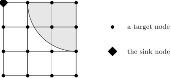
in the sequel, or randomly in a square area. This two kinds of deployment define planar graphs where X represents the vertices (targets). In the case of grid graphs,
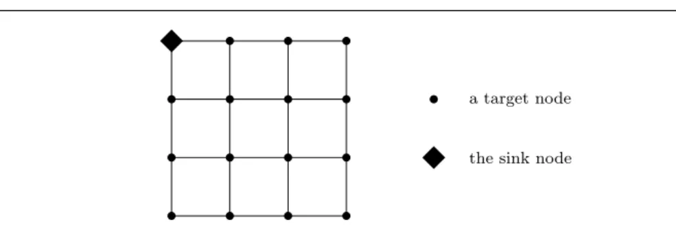
a target node
the sink node
Fig. 1: Square grid with 4 rows and 4 columns.
the vertices are deployed following a square grid with unitary distances (d= 1) with
nrows andncolumns, i.e.,|X|=n2. Figure 1 shows such a grid. We choose to focus on square grid graphs, which are close to 4−regular low density graphs, since these graphs appear to be among the most challenging instances in terms of exact resolution, and have up to now been the subject of very few specific works, as noticed in (Reich 2016). Random graphs are also considered in order to evaluate the performance of the mathematical programming formulations we propose for the MCC and MCkC problems on graphs where targets are not deployed following a regular pattern. In the rest of this paper, we consider that bothGse andGco are connected digraphs.
The remainder of the paper is organized as follows: Section 2 presents related works. In the case where targets are located via a regular pattern, Section 3 proposes a sufficient condition on integer radii Rco and Rse according to which coverage of targets implies connectivity. After recalling a recent model dedicated to grid graphs, Section 4 describes two formulations that can be used for general graphs. Section 5 compares the three formulations through computational experiments on grids and random graphs. Section 5 extends our computational experiments to a generalization of the MCC problem: the Minimum Connectedk-Coverage problem. Finally, Section 6 concludes this paper.
2 Related work
In (Lucena et al 2010), Lucena et al. propose enhanced formulations of the MLST problem related to a previous edge-vertex formulation and polyhedron investigations by Fujie (Fujie 2003), (Fujie 2004) and Gon¸calves et al. (Gon¸calves et al 2011). These two prior works did not provide experimental results of their formulations while the work by Lucena et al. shows detailed comparisons of several algorithms based on these formulations. Gendron et al. (Gendron et al 2014) later extended this study by presenting a branch-and-cut algorithm and a Benders decomposition algorithm based on the same formulation. So far they have obtained the best exact results since they succeeded in solving problems with 200 vertices and low edge density. The authors of (Reis et al 2015) propose a flow based formulation for the MLST problem. While this formulation is very simple, it gives roughly similar results to the ones exhibited by Lucena et al. (Lucena et al 2010).
Fan and Watson (Fan and Watson 2012) focus on several mixed integer linear for-mulations for the MCDS problem: Miller-Tucker-Zemlin (MTZ) formulation, Martin constraints, and flow formulations. They have succeeded in solving a 300 vertices in-stance with low density. Finally, Rebai et al. (Rebai et al 2015) propose a formulation inspired by path constraints and focus their studies on the MCC problem in square grid graphs. To our knowledge, the complexity of this problem is unknown in square grid graphs. In a recent work (Rebai et al 2016), Rebai et al. have considered another problem close to the previous one, called critical grid coverage problem, which is an
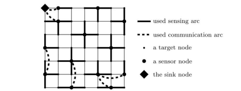
used sensing arc used communication arc a target node
a sensor node the sink node
Fig. 2: A non-connected coverage solution in a 7x7 Grid with Rse= 1 and Rco= 2.
NP-Complete problem (Ke et al 2011). In this problem, only a given part of the square grid, called critical cells, have to be covered by the sensors and not all the grid. The authors proposed two mixed integer linear programming models, which are able to compute optimal solutions for square grid graphs of size up to 15×15.
3 When coverage implies connectivity
This section deals with a sufficient condition on integer radii Rco and Rse (with
Rco≥ Rse) such that a dominating set forGse induces a connected subgraph inGco
when targets are deployed according to a regular pattern. We mean byd-regular pattern
that every target is at an Euclidean distanced ≤ Rse from all the other targets in its sensing neighbourhood.
Wang et al. (Wang et al 2003) have studied the total coverage of the area and the connectivity for the sensors placement with no restriction on Rse and Rco. They have proven that when the communication radius Rco is at least twice the sensing rangeRse, the connectivity is automatically achieved when the total coverage of the area is reached. This result cannot be generalised to the case of a discrete set of targets coverage. Indeed, we prove in Propositions 1 and 2 that we need a larger communication radius than twice the sensing radius in order to get the connectivity ensured by the covering.
Proposition 1 In a wireless sensor network R= (Gse, Gco)where targets are deployed according to a square grid, if Rco= 2Rsethen a dominating set for Gsedoes not necessarily induce a connected subgraph in Gco.
Proof We propose to build a dominating set forGsethat does not induce a connected subgraph in Gcowhen Rco= 2Rse.
Figure 2 presents an example of sensors placement which is a dominating set for a grid 7×7 when Rse = 1. WhenRco = 2Rse = 2, this subset of sensors induces a subgraph ofGco which is composed of 8 connected components and not a single one. This subgraph of Gco is illustrated in Figure 2 where communication links between sensors are shown by dashed lines. ut
In the next proposition, we propose an extension of Wang et al’s result to the discrete case of target coverage when radii are integers and every pair of adjacent targets in Gse are at distanced from each other, i.e., we consider graphs where the targets are deployed following a d-regular pattern.
Proposition 2 In a wireless sensor network R= (Gse, Gco)where targets are deployed according to a d-regular pattern, if Rco≥2Rse+d then a dominating set of Gse automat-ically induces a connected subgraph in Gco.
Proof We suppose that Rco = 2Rse+d. Consider a sensor network R= (Gse, Gco) and a dominating setS of Gse. We suppose that the subgraph induced by S is not connected inGco. So, there exists at least one pair of adjacent targets inGse calleda
andb(such thatd(a, b) =d) that are not covered by the same connected component. Consider x (resp. y) a sensor that covers the target a (resp. b) which belongs to a connected component namedCa (resp.Cb).
We haved(x, a)≤ Rseandd(y, b)≤ Rse. According to triangular inequalities respected by Euclidean distances,d(x, y)≤ d(x, a) +d(a, b) +d(b, y). So,d(x, y)≤2Rse+d, which means thatCaandCbare connected, this leads to a contradiction with our hypothesis.
u t
From Propositions 1 and 2, we can deduce the following result.
Corollary 1 In a wireless sensor network R = (Gse, Gco) where targets are deployed according to a d-regular pattern, if Rco≥2Rse+d then every solution for the k-coverage problem is also a solution for the connected k-coverage problem.
Proof Observe first that every solution for the k-coverage problem in Gse is also a solution for the 1-coverage problem (or dominating set problem). So, we can apply Proposition 2 to conclude that every solution induces a connected subgraph inGco.
u t
Note that for grids, coverage implies connectivity whenRco≥2Rse+ 1.
4 Three Mixed Integer Linear Programming formulations of MCC
We first recall the formulation in (Rebai et al 2015) which is dedicated to grids. We then present two different formulations based on single commodity flow and MTZ constraints respectively.
4.1 Model of Rebai et al. (Rebai et al 2015) (MIP1)
The model proposed in (Rebai et al 2015) is only defined for grid graphs. It relies on the distinction between two types of paths connecting a sensor to the sink:directand
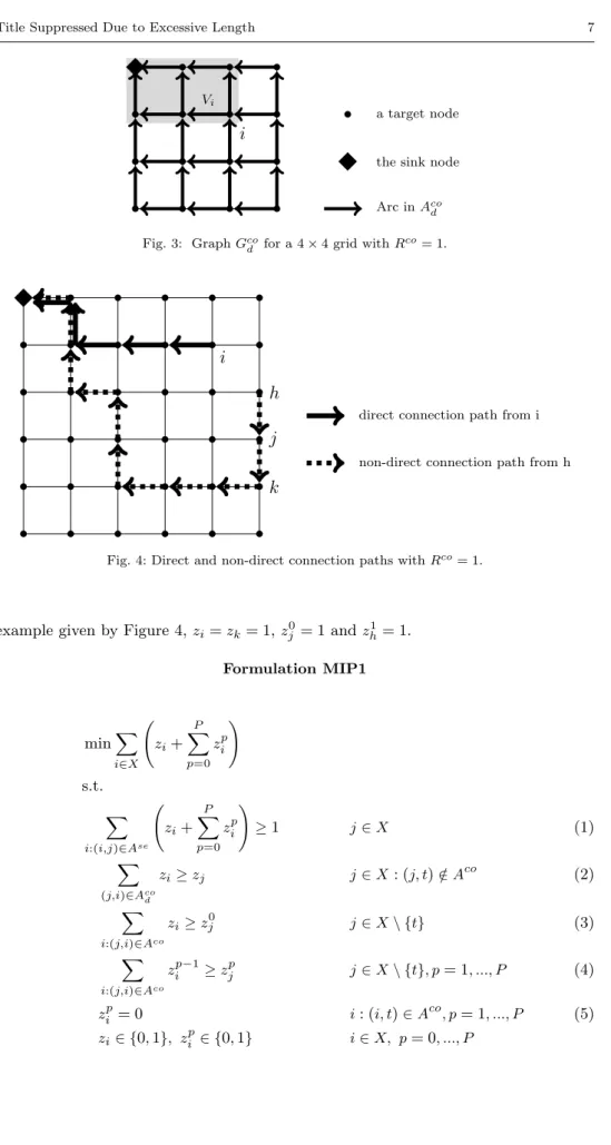
non-direct connection paths. For any node i, consider the smallest rectangle on the grid that contains this node and the sinkt. Let Vi denotes the set of nodes located
inside this rectangle. LetGcod = (X, Acod ) denotes the partial subgraph of Gco where, for every j0 ∈ X\{t}, only the arcs (j0, j) where j ∈ Vj0 are kept. Figure 3 gives an
example ofGcod for a 4×4 grid. A path from a nodeito the sink is said to be adirect connection pathif it only uses arcs inAcod . Otherwise, if the path includes at least one arc that does not belong toAcod , it is said to be annon-direct connection path. Examples of direct and non-direct connection paths are illustrated by Figure 4. It was shown in (Rebai et al 2015) that the length (number of arcs) of a non-direct connection path in an optimal solution can be upper bounded byP=d2(Rn−co1)e. WhenRco= 1,P can
be viewed as the maximal Manhattan distance inAco, i.e., the sum of the number of rows and the number of columns of the grid.
The model proposed in (Rebai et al 2015) is given in Formulation MIP1. Fori ∈ X, the binary variablezi is equal to 1 if a sensor is placed on node iand there exists a
direct connection path inGcod from this sensor to the sink, and 0 otherwise. Fori ∈ X
andp ∈ {0, ..., P }, the binary variablezip is equal to 1 if a sensor placed on nodeiis located atpsensors from a direct connection path to the sink, and 0 otherwise. It can be noted that zi0 = 1 means that there exists (i, j)∈ Aco such thatzj = 1. On the
Vi
i
a target node
the sink node
Arc in Aco d
Fig. 3: Graph Gco
d for a 4 × 4 grid with Rco= 1.
i
j
h
k
direct connection path from i
non-direct connection path from h
Fig. 4: Direct and non-direct connection paths with Rco= 1.
example given by Figure 4,zi=zk= 1,zj0= 1 andzh1= 1.
Formulation MIP1 minX i∈X zi+ P X p=0 zip ! s.t. X i:(i,j)∈Ase zi+ P X p=0 zip ! ≥1 j ∈ X (1) X (j,i)∈Aco d zi≥ zj j ∈ X: (j, t)∈ A/ co (2) X i:(j,i)∈Aco zi≥ z0j j ∈ X \ {t} (3) X i:(j,i)∈Aco zip−1≥ zpj j ∈ X \ {t}, p= 1, ..., P (4) zpi = 0 i: (i, t)∈ Aco, p= 1, ..., P (5) zi∈ {0,1}, zip∈ {0,1} i ∈ X, p= 0, ..., P
The objective function measures the total number of sensors placed on the grid. Indeed, the expression zi+
P
P
p=0 zpi
!
is equal to 1 if a sensor is placed on nodeiand 0 otherwise. Constraints (1) are covering constraints. They mean that each node of the grid must belong to the neighbourhood of at least one sensor. With Constraints (2) one can check that a sensor placed on node j has a direct connection path to the sink if there exists a successoriofjin Gcod that has a direct connection path to the sink. Similarly, Constraints (3) are related to non-direct connection paths. A sensor placed on node j has an non-direct connection path to the sink if a sensor placed on node ibelongs to its communication neighbourhood and has a direct connection path to the sink. Constraints (4) implement the induction condition on non-direct connection paths. A sensor placed on node j is located at a distance of p nodes from a direct connection path to the sink if at least one sensor in its communication neighbourhood is located at a distance of (p −1) nodes from a direct connection path. Finally, Constraints (5) ensure that if a sensor is placed on a node iwhich has the sink in its communication neighbourhood then this sensor is connected to the sink via the arc (i, t).
For an×ngrid, the number of variables and the number of constraints are bounded byO(|X|p
|X|).
Below, we present two models that can be used for general graphs. Let us first recall that a solution of the MCC problem can be viewed as a subset S ofX. SetS
represents the nodes where sensors will be placed. Each sensor in S communicates with the sinktthrough a path inAco joining nodes fromS. Moreover, each nodeiin
X \ {t}is covered by a sensor located either onior on one of its neighbours inGse. This solutionS can be represented by a directed spanning tree of the grid rooted at
t. In the in-tree, a node with no sensor is connected to a sensor by an arc inAseand then this sensor is connected to the sink t through a path of sensors connected by communication arcs inAco.
4.2 Single Commodity Flow Model (MIP2)
The Single Commodity Flow (SCF) model that we describe hereafter was introduced by Gavish (Gavish 1982) for solving the directed minimal spanning tree problem and recently used by Reis et al. for the MLST problem (Reis et al 2015) and Fan and Watson (Fan and Watson 2012) for the MCDS problem. It is based on the idea that every node ofXwill send one unit of flow towards the sink nodet. The flow is conveyed by arcs fromAseand fromAco. A node with no sensor will send a unit of flow through an arc inAse. A node with a sensor will gather incoming flows fromAse andAcoand send all through a unique outgoing arc inAco. For this model (given in Formulation MIP2), we need to define the following variables:
– xi,i ∈ X, is equal to 1 if a sensor is placed on nodeiand 0 otherwise,
– fijco, (i, j)∈ Aco, is the amount of communication flow on arc (i, j) from nodei
to node j, if a sensor on i communicates with a sensor on j. Variable fijco is a
non-negative real number, upper-bounded by the number of nodes inX \ {t}, i.e.,
n2−1,
– fijse, (i, j)∈ Ase, is the amount of sensing flow from nodeito nodej, if no sensor
is placed on i and the sensing flow from i is sent to the sensor on node j. It is equal to 0 otherwise. It follows from the definition that 0≤ fijse≤1.
We also need to define the following notations.Miis any large enough integer that
Formulation MIP2 min X i∈X xi s.t. X
i∈X:(i,t)∈Aco
xi≥1 (6) xi+ X j∈X:(i,j)∈Ase xj≥1 i ∈ X \ {t} (7) X j∈X:(j,t)∈Aco fjtco=n2−1 (8) xi+ X j∈X:(i,j)∈Ase fijse= 1 i ∈ X \ {t} (9) X j∈X:(j,i)∈Aco fjico+ X j∈X:(j,i)∈Ase fjise+xi = X j∈X:(i,j)∈Aco fijco i ∈ X \ {t} (10) X j∈X:(i,j)∈Aco fijco≤ Mixi i ∈ X \ {t} (11) X j∈X:(j,i)∈Ase fjise≤(δ−i −1)xi i ∈ X \ {t} (12) xi∈ {0,1} i ∈ X 0≤ fijco≤ n2−1, fijco∈R (i, j)∈ Aco 0≤ fijse≤1, fijse∈R (i, j)∈ Ase
With Constraints (6), the coverage of the sink nodet by one of its predecessor nodes in the communication graph is satisfied. The coverage of the other nodes is satisfied by Constraints (7). Constraint (8) expresses that the incoming communica-tion flow at the sink node is the aggregacommunica-tion of flows sent by each node in X \ {t}. Constraints (9) ensure that if a sensor is placed on nodei(xi= 1), the sensing outflow
fromiinAse is 0. But, if no sensor is placed oni(xi = 0), nodeisends one unit of
flow on a unique sensing arc in Ase. Constraints (10) ensure the connectivity of the solution by flow conservation: if no sensor is placed on node i, the incoming – com-munication and sensing – flow is equal to outgoing comcom-munication flow. However, if a sensor is located on nodei, the outgoing communication flow is equal to the incoming flow plus one. Constraints (11) ensure that if no sensor is placed on node ithen its outgoing communication flows are equal to 0. Finally, Constraints (12) mean that if no sensor is placed on node i then its incoming sensing flow is equal to 0. On the contrary, if a sensor is placed on nodeithen the incoming sensing flow is the number of non-sensor nodes that useiand this number is limited by (δ−i −1).
The number of variables is bounded byO(|Aco|) (since we make the assumption
Rse≤ Rco) and the number of constraints byO(|X|).
4.3 Formulation based on Miller-Tucker-Zemlin Model (MIP3)
Here, we change the way of handling the connectivity requirement. The model of this subsection is inspired from the Miller-Tucker-Zemlin (MTZ) formulations of spanning
trees and other graph applications. MTZ constraints have been initially used to solve the travelling salesman problem (Miller et al 1960).
For this model (given in Formulation MIP3), we need to define the following variables:
– xi,i ∈ X, is the same variable as above,
– yijco, (i, j)∈ Aco, is also a binary variable, equal to 1 if and only if a communication link fromitojis used from a sensor placed on nodeito a sensor placed on node
j.
– yijse, (i, j) ∈ Ase, is a binary variable, equal to 1 if and only if a node i, with
no sensor, is covered by a sensor placed on node j through the arc (i, j). With these definitions of theyco andysevariables, the set of arcs such that one of these variables is equal to 1 should build a spanning oriented tree of X, rooted att.
– Li,i ∈ X, counts the number of sensors in the path of sensors fromito the sink
node if a sensor is placed on nodei. IfLt= 0,Lican be defined as a non-negative
real number. Formulation MIP3 min X i∈X xi s.t. Constraints (6), (7) X j∈X:(i,j)∈Aco ycoij =xi i ∈ X \ {t} (13) xi+ X j∈X:(i,j)∈Ase yseij = 1 i ∈ X \ {t} (14) X (j,i)∈Ase yjise+ X (j,i)∈Aco ycoji ≤(δi−−1)xi i ∈ X \ {t} (15) Lt= 0 (16) Li≥ Lj+ 1−(n2−1)(1− yijco) (i, j)∈ A co (17) Li≥0 i ∈ X xi∈ {0,1} i ∈ X ycoij ∈ {0,1} (i, j)∈ A co yseij ∈ {0,1} (i, j)∈ Ase
Constraints (13) say that the number of outgoing communication arcs from a non-sink nodeiis equal to 1 ifireceives a sensor and 0 otherwise. Constraints (14) say that the number of outgoing sensing arcs from a non-sink nodeiis equal to 0 if
i receives a sensor and 1 otherwise. Observe that Constraints (14) and (9), as well as variablesyijse andfijse, are actually the same. Constraints (15) ensure that a
non-sink node i has incoming arcs only if a sensor is placed on i and that the number of incoming arcs ofi is limited by its in-degree minus one. Constraints (17) are the original Miller-Tucker-Zemlin constraints to guarantee that the solutions are directed subtrees rooted attwhich span selected sensors in Gco.
5 Comparison of the three MIP formulations
The objective of our computational experiments is to compare the formulations on two kinds of instances : grid sensor networks and randomly generated graphs. We coded the MIP formulations by use of the AMPL mathematical programming mod-eller (Fourer et al 1993) and solve the mathematical programming problems by use of Cplex12.6.2(IBM-ILOG 2014) with a time limit of 1 hour. All our instances have been tested on an Intel(R) Xeon(R) CPU E5-2680 v3 2.50GHz with 48 CPU and with 64 GB of RAM.
5.1 Results for the MCC problem
5.1.1 Grid sensor networks
All the considered instances in this section are grids with n rows and n columns, denoted Gn, with different values of Rco andRse. The sink nodetis located at the
left high corner.
We performed computational experiments on several instances of Gn withn= 6
to 15, Rse varying from 1 to 3 andRse ≤ Rco ≤2Rse (see Proposition 2 in Section
3). Table 1 summarizes the number of decision variables and constraints for each formulation MIP1, MIP2, and MIP3, as described in the previous section. The number of variables of MIP2 and MIP3 depends on |Aco|, in other words it depends on the value of Rco. We can also observe that the number of constraints of MIP3 actually depends on |Aco|. Moreover, the out-degree of a node x in Gco, denoted by δ+x, is
upper bounded by (2Rco+ 1)2 (the number of nodes in the square of side length 2Rco
which contains the circle of radiusRco). Thus,|Aco|is bounded byO(|X| ×(Rco)2).
Number of MIP1 MIP2 MIP3 Variables O(|X|p|X|) O(|X|(Rco)2) O(|X|(Rco)2) Constraints O(|X|p|X|) O(|X|) O(|X|(Rco)2)
Table 1: Number of variables and constraints for each formulation
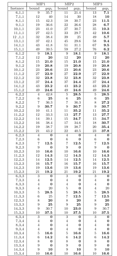
Our results are detailed in Table 2 as well as in Table 3 where the first column
Instance gives the characteristics of the instance in the format n Rse Rco. The best results are emphasized in bold.
In Table 2, the next columns give, for each formulation MIP1, MIP2, and MIP3, (i) the bound computed as the optimal value of the continuous relaxation of the formulation, obtained by solving specifically the LP-relaxation of the model and (ii) the initial gap, denoted by gapi, between the best known solution value, denoted
bkn, computed by one of the three formulations and the boundas a percentage, i.e., precisely, bkn−boundbkn ∗100.
For instances, whenRse=Rco= 1, we can observe that MIP3 always provides the best bound by continuous relaxation. The average gap on these 10 instances is equal to about 37.2% with MIP1, 26.5% with MIP2, and 8.6% with MIP3. When Rse= 1 andRco= 2, MIP1, MIP2 and MIP3 provide similar bounds with an average gap of 22.6%. Again for Rse = Rco = 2, MIP3 provides globally better bounds. However, for the remaining instances with (Rse, Rco) = (2,3), (3,3), and (3,4), the difference between the three bounds is not enough significant while we observe that the bounds become stronger.
In Table 3, we provide the results of the branch-and-bound phases of the three formulations. For each formulation MIP1, MIP2, and MIP3, we give (i) the CPU time
MIP1 MIP2 MIP3 Instance bound gapi bound gapi bound gapi
6 1 1 9 35.7 11 21.4 13 7.1 7 1 1 12 40 14 30 18 10 8 1 1 15 42.3 18 30.7 23 11.5 9 1 1 19 36.6 22 26.6 28 6.7 10 1 1 23 41.0 27 30.7 35 10.3 11 1 1 27 42.5 33 29.7 42 10.6 12 1 1 32 38.4 39 25 49 5.7 13 1 1 37 42.1 45 29.6 58 9.4 14 1 1 43 41.8 51 31.1 67 9.5 15 1 1 49 39.5 59 27.2 76 6.2 6 1 2 9 18.1 9 18.1 9 18.1 7 1 2 12 20 12 20 12 20 8 1 2 15 21.0 15 21.0 15 21.0 9 1 2 19 20.8 19 20.8 19 20.8 10 1 2 23 20.6 23 20.6 23 20.6 11 1 2 27 22.9 27 22.9 27 22.9 12 1 2 32 23.8 32 23.8 32 23.8 13 1 2 37 24.4 37 24.4 37 24.4 14 1 2 43 23.2 43 23.2 43 23.2 15 1 2 49 24.6 49 24.6 49 24.6 6 2 2 4 42.8 5 28.5 5 28.5 7 2 2 6 25 6 25 6 25 8 2 2 7 36.3 7 36.3 8 27.2 9 2 2 9 30.7 9 30.7 9 30.7 10 2 2 10 41.1 11 35.2 11 35.2 11 2 2 12 33.3 13 27.7 13 27.7 12 2 2 14 39.1 15 34.7 15 34.7 13 2 2 16 38.4 17 34.6 18 30.7 14 2 2 19 38.7 19 38.7 20 35.4 15 2 2 21 43.2 22 40.5 23 37.8 6 2 3 4 0 4 0 4 0 7 2 3 6 0 6 0 6 0 8 2 3 7 12.5 7 12.5 7 12.5 9 2 3 9 0 9 0 9 0 10 2 3 10 16.6 10 16.6 10 16.6 11 2 3 12 14.3 12 14.3 12 14.3 12 2 3 14 12.5 14 12.5 14 12.5 13 2 3 16 15.7 16 15.7 16 15.7 14 2 3 19 13.6 19 13.6 19 13.6 15 2 3 21 19.2 21 19.2 21 19.2 6 3 3 3 0 3 0 3 0 7 3 3 4 0 4 0 4 0 8 3 3 4 0 4 0 4 0 9 3 3 4 20 5 0 4 20 10 3 3 5 28.5 5 28.5 5 28.5 11 3 3 6 25 7 12.5 7 12.5 12 3 3 8 20 8 20 8 20 13 3 3 9 25 9 25 9 25 14 3 3 9 30.7 10 23.0 9 30.7 15 3 3 10 37.5 10 37.5 10 37.5 6 3 4 3 0 3 0 3 0 7 3 4 4 0 4 0 4 0 8 3 4 4 0 4 0 4 0 9 3 4 4 0 4 0 4 0 10 3 4 5 16.6 5 16.6 5 16.6 11 3 4 6 14.2 6 14.2 6 14.2 12 3 4 8 0 8 0 8 0 13 3 4 9 0 9 0 9 0 14 3 4 9 10 9 10 9 10 15 3 4 10 16.6 10 16.6 10 16.6
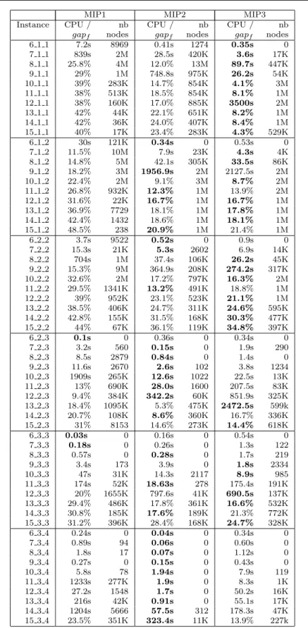
Instance CPU / nb CPU / nb CPU / nb gapf nodes gapf nodes gapf nodes
6 1 1 7.2s 8969 0.41s 1274 0.35s 0 7 1 1 839s 2M 28.5s 420K 3.6s 17K 8 1 1 25.8% 4M 12.0% 13M 89.7s 447K 9 1 1 29% 1M 748.8s 975K 26.2s 54K 10 1 1 39% 283K 14.7% 854K 4.1% 3M 11 1 1 38% 513K 18.5% 854K 8.1% 1M 12 1 1 38% 160K 17.0% 885K 3500s 2M 13 1 1 42% 44K 22.1% 651K 8.2% 1M 14 1 1 42% 36K 24.0% 407K 8.4% 1M 15 1 1 40% 17K 23.4% 283K 4.3% 529K 6 1 2 30s 121K 0.34s 0 0.53s 0 7 1 2 11.5% 10M 7.9s 23K 4.3s 4K 8 1 2 14.8% 5M 42.1s 305K 33.5s 86K 9 1 2 18.2% 3M 1956.9s 2M 2127.5s 2M 10 1 2 22.4% 2M 9.1% 3M 8.7% 2M 11 1 2 26.8% 932K 12.3% 1M 13.9% 2M 12 1 2 31.6% 22K 16.7% 1M 16.7% 1M 13 1 2 36.9% 7729 18.1% 1M 17.8% 1M 14 1 2 42.4% 1432 18.6% 1M 18.1% 1M 15 1 2 48.5% 238 20.9% 1M 21.4% 1M 6 2 2 3.7s 9522 0.52s 0 0.9s 0 7 2 2 15.3s 21K 5.3s 2602 6.9s 14K 8 2 2 704s 1M 37.4s 106K 26.2s 45K 9 2 2 15.3% 9M 364.9s 208K 274.2s 317K 10 2 2 32.6% 2M 17.2% 797K 16.3% 2M 11 2 2 29.5% 1341K 13.2% 491K 18.8% 1M 12 2 2 39% 952K 23.1% 523K 21.1% 1M 13 2 2 38.5% 406K 24.7% 311K 24.6% 595K 14 2 2 42.8% 155K 31.5% 168K 30.3% 477K 15 2 2 44% 67K 36.1% 119K 34.8% 397K 6 2 3 0.1s 0 0.36s 0 0.34s 0 7 2 3 3.2s 560 0.15s 0 1.9s 290 8 2 3 8.5s 2879 0.84s 0 1.4s 0 9 2 3 11.6s 2670 2.6s 102 3.8s 1234 10 2 3 1909s 265K 12.6s 1022 22.5s 13K 11 2 3 13% 690K 28.0s 1600 207.5s 83K 12 2 3 9.4% 384K 342.2s 60K 851.9s 325K 13 2 3 18.4% 1095K 5.3% 475K 2472.5s 599k 14 2 3 20.7% 108K 8.6% 360K 16.7% 336K 15 2 3 31% 8153 14.6% 273K 14.4% 618K 6 3 3 0.03s 0 0.16s 0 0.54s 0 7 3 3 0.18s 0 0.26s 0 1.3s 122 8 3 3 0.57s 0 0.28s 0 1.7s 219 9 3 3 3.4s 173 3.9s 0 1.8s 2334 10 3 3 47s 31K 14.3s 2117 8.9s 985 11 3 3 174s 52K 18.63s 278 175.4s 191K 12 3 3 20% 1655K 797.6s 41K 690.5s 137K 13 3 3 29.4% 486K 17.8% 361K 16.6% 532K 14 3 3 30.8% 185K 17.6% 189K 21.3% 772K 15 3 3 31.2% 396K 28.4% 168K 24.7% 328K 6 3 4 0.24s 0 0.04s 0 0.34s 0 7 3 4 0.89s 94 0.06s 0 0.60s 0 8 3 4 1.8s 17 0.07s 0 1.12s 0 9 3 4 0.27s 0 0.15s 0 0.43s 0 10 3 4 5.8s 78 1.94s 0 7.9s 119 11 3 4 1233s 277K 1.9s 0 8.3s 1K 12 3 4 27.2s 1548 1.7s 0 50.2s 16K 13 3 4 216s 42K 0.91s 0 55.1s 17K 14 3 4 1204s 5666 57.5s 312 178.3s 47K 15 3 4 23.5% 351K 323.4s 11K 13.9% 227k
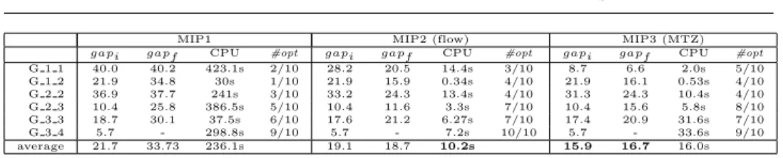
MIP1 MIP2 (flow) MIP3 (MTZ) gapi gapf CPU #opt gapi gapf CPU #opt gapi gapf CPU #opt G 1 1 40.0 40.2 423.1s 2/10 28.2 20.5 14.4s 3/10 8.7 6.6 2.0s 5/10 G 1 2 21.9 34.8 30s 1/10 21.9 15.9 0.34s 4/10 21.9 16.1 0.53s 4/10 G 2 2 36.9 37.7 241s 3/10 33.2 24.3 13.4s 4/10 31.3 24.3 10.4s 4/10 G 2 3 10.4 25.8 386.5s 5/10 10.4 11.6 3.3s 7/10 10.4 15.6 5.8s 8/10 G 3 3 18.7 30.1 37.5s 6/10 17.6 21.2 6.27s 7/10 17.4 20.9 31.6s 7/10 G 3 4 5.7 - 298.8s 9/10 5.7 - 7.2s 10/10 5.7 - 33.6s 9/10 average 21.7 33.73 236.1s 19.1 18.7 10.2s 15.9 16.7 16.0s
Table 4: Synthesis of numerical results for MIP1, MIP2 and MIP3
(in seconds) for the whole branch-and-bound phase when it stops before reaching the time limit, or, alternatively, the final gap denoted by gapf when the time limit is
reached, and (ii) the number of generated nodes.
Here again, we can observe different behaviours of the models depending onRse
andRcobut the most striking observation is that with MIP1, we can solve 26 instances over the 60 considered within the time limit of one hour, while MIP2 can solve 34 instances and MIP3, two more instances than MIP2. Focusing on the instances where
Rse =Rco = 1, we can observe that MIP3 either solves the instances faster, or can solve instances that neither MIP1 nor MIP2 can solve within the time limit, or reaches the time limit with a better final gap. Concerning the other pairs (Rse, Rco), the per-formances of MIP2 and MIP3 seem rather similar. Our final observation is that MIP1 is always outperformed either by MIP2 or MIP3 on 55 instances. Table 4 summarizes our numerical results. It presents, for each pair (Rse, Rco), the average initial and final gaps (in percentage). The averagegapf is computed over the subset of instances not
solved by both formulations, as a consequence gapf is not always lower than gapi.
Also, the average CPU time (in seconds) for the whole branch-and-bound phase is computed only for instances solved by the three formulations. If we focus on MIP2 and MIP3, Table 4 shows that MIP3 slightly outperforms MIP2 over 3 criteria: MIP3 solves three more instances to optimality and provides better average initial and final gaps. However, if the average CPU time for the whole branch-and-bound phase is computed only for instances solved by MIP2 and MIP3, it is divided by 1.6 in favour of MIP2.
In the following, we do not take into account MIP1 model since it is dedicated to grid sensor networks.
5.1.2 Random sensor networks
In this section, we propose to examine the performance of our two models for randomly generated graphs.
Our instances are generated as follows. We first defined a square area of sidesin the euclidean plane with the origin of the euclidean plane as the left low corner of the square. n targets were then randomly generated with a uniform distribution in this square. Givensandn, we generated sensing and communication graphs relatively to
Rse varying from 1 to 3 and Rse ≤ Rco ≤ 2Rse. We repeated the generation until the graphs become connected. For each pair (s,n), we selected five random targets placement. The sink nodetis always located at the origin of the euclidean plan. An illustration of the generation of 50 targets in a square of side 4 is given in Figure 5. In this example, an optimal solution of sensors placement is represented by twelve rhombi.
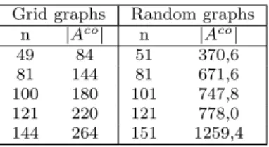
Table 5 compares the average number of arcs of our testbed instances for Rco =
Rse= 1 versus grid instances, and shows the large density of our instances.
Our results are detailed in Table 6 where the first column Instances gives the characteristics of the instance in the formatn s Rse Rco. The columnCPUlists the
Fig. 5: n=50 targets generated in a square of side s = 4.
Grid graphs Random graphs n |Aco| n |Aco| 49 84 51 370,6 81 144 81 671,6 100 180 101 747,8 121 220 121 778,0 144 264 151 1259,4
Table 5: Comparison of |Aco| between grid and random graphs when Rco= Rse= 1
average CPU time for instances solved to optimality within one hour. The best results are emphasized in bold.
Flow model MIP2 MTZ model MIP3
Instances gapi% gapf% CPU #solved gapi% gapf% CPU #solved
G 50 4 1 1 28.8 - 1.01s 5/5 36.4 - 17.4s 5/5 G 50 4 1 2 0.0 - 0.04s 5/5 0.0 - 0.76s 5/5 G 80 5 1 1 33.3 - 13.1s 5/5 37.9 - 747,6s 5/5 G 80 5 1 2 0.00 - 0.17s 5/5 0.00 - 1.43s 5/5 G 100 6 1 1 32.9 - 42.7s 5/5 37.1 11.05 1999.9s 1/5 G 100 6 1 2 0.00 - 0.23s 5/5 0.00 - 1.95s 5/5 G 120 7 1 1 40.8 8.3 258.1s 4/5 41.3 19.9 3600s 0/5 G 120 7 1 2 0.0 - 0.27s 5/5 0.0 - 3.0s 5/5 G 120 7 2 2 21.1 - 63.5s 5/5 28.3 - 341.0s 5/5 G 120 7 2 3 8.6 - 3.00s 5/5 8.6 - 5.2s 5/5 G 150 7 1 1 35.6 7.9 866.4s 2/5 39.9 20.4 3600s 0/5 G 150 7 1 2 0.0 - 0.24s 5/5 0.0 - 2.7s 5/5 G 150 7 2 2 21.9 - 134.1s 5/5 26.7 17.6 203.6s 3/5 G 150 7 2 3 2.9 - 2.4s 5/5 5.7 - 7.3s 5/5
Table 6: Synthesis of Numerical results for random sensor networks
For the whole of instances, MIP2 (flow model) outperforms MIP3 (MTZ model) over all criteria. Over the 70 tested instances, 66 (resp. 54) are solved to optimality within one hour by MIP2 (resp. MIP3) and the MIP solving for instances solved by both models needs only 12,6 seconds in average for MIP2 compared to 121,1 seconds for MIP3. Thus, MIP2 is ten times faster than MIP3. This can be partly explained by the fact that the average initial gapgapi provided by MIP2 is better than for MIP3:
16% versus 19%. Finally, the average final gapgapf computed for the instances, not
solved within one hour by both models, is 2,6 times larger for MIP3 than for MIP2 (8.1% vs 21.5%). Important density of random graphs can also explain the superiority of MIP2 over MIP3, since the number of constraints of MIP3 depends on|Aco|.
5.2 Results for the MCkC problem withk= 2 or 3
In this section, we consider a generalization of the MCC problem: the Minimum Con-nected k-Coverage (MCkC) problem where a positive integer k defines the coverage multiplicity of the targets.
In order to satisfy thek-coverage constraint, our two models MIP2 and MIP3, dedi-cated to the MCC problem, can easily be modified by replacing the 1-coverage con-straint
xi+
X
j∈X:(i,j)∈Ase
xj≥1 ∀i ∈ X \ {t}
by thek-coverage constraint
xi+
X
j∈X:(i,j)∈Ase
xj≥ k ∀i ∈ X \ {t}
5.2.1 Grid sensor networks
For square grids and a givenRse, it existskmaxsuch that, for allk > kmax, the MCkC
problem does not admit a solution. For example, for Rse = 1, a target located in a corner of the grid has a sensing neighbourhood of cardinality 3. So, this target cannot be covered more than three times. We conclude tokmax= 3 whenRse= 1. Figure 6
illustrates the case kmax= 6 whenRse = 2. Table 7 listskmax forRse varying from
1 to 4.
a target node
the sink node
Fig. 6: Sensing neighbourhood for a target in a corner of the grid when Rse= 2.
Rse kmax
1 3
2 6
3 11 4 17
Table 7: Maximal values for k
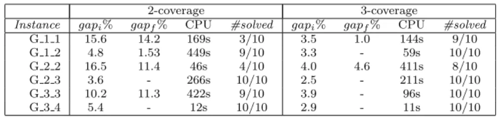
Numerical results for Grid sensor networks are summarized in Table 8 for MIP2 and in Table 9 for MIP3, in which the best results are emphasized in bold. Note that the values presented for each pair (Rse,Rco) in these two tables are average values over the ten grid instances. MIP2 (based on single flow commodity) solves three more instances than MIP3 (based on MTZ constraints) for k= 2 and two more instances fork= 3. For both models, two behaviours are observed. First, whenk= 2, instances withRse=Rcoare more difficult to solve. Indeed, initial gaps are larger: 15.3% (resp.
14.1%) in average for MIP2 (resp. MIP3), whereas, for instances withR =R + 1, the average gap is reduced to 4.5%. Secondly, the Minimum Connected k-Coverage Problem is easier to solve when k is larger. Indeed, for k = 3, MIP2 (resp. MIP3) solves 59 (resp. 57) of the 60 instances within the time limit of one hour. Those observations can be explained by the fact that less extra sensors are necessary to ensure connectivity whenk andRco increase.
2-coverage 3-coverage
Instance gapi% gapf% CPU #solved gapi% gapf% CPU #solved
G 1 1 18.1 12.7 1034s 3/10 3.5 - 21s 10/10 G 1 2 4.9 - 280s 10/10 3.3 - 22s 10/10 G 2 2 18.5 11.4 212s 5/10 3.5 2.4 140s 9/10 G 2 3 3.7 - 15s 10/10 2.5 - 44s 10/10 G 3 3 9.4 - 568s 10/10 3.7 - 16s 10/10 G 3 4 5.4 - 8s 10/10 2.9 - 3s 10/10 Table 8: Numerical results for minimum connected k-coverage with adapted flow model (MIP2).
2-coverage 3-coverage
Instance gapi% gapf% CPU #solved gapi% gapf% CPU #solved
G 1 1 15.6 14.2 169s 3/10 3.5 1.0 144s 9/10 G 1 2 4.8 1.53 449s 9/10 3.3 - 59s 10/10 G 2 2 16.5 11.4 46s 4/10 4.0 4.6 411s 8/10 G 2 3 3.6 - 266s 10/10 2.5 - 211s 10/10 G 3 3 10.2 11.3 422s 9/10 3.9 - 96s 10/10 G 3 4 5.4 - 12s 10/10 2.9 - 11s 10/10 Table 9: Numerical results for minimum connected k-coverage with adapted MTZ model (MIP3).
5.2.2 Random sensor networks
Numerical results for Random sensor networks are summarized in Table 10 for the minimum connected 2-coverage problem. Table 11 sums up the results obtained for the set of graph instances with 150 nodes. The best results are emphasized in bold.
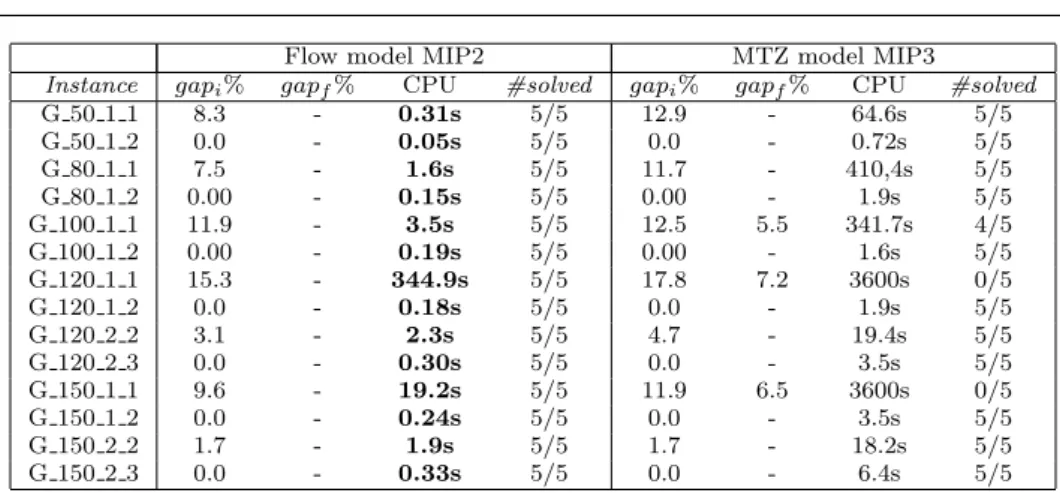
We have the same observation than for grid square instances. Indeed, whenk= 2, instances withRse=Rcoare more difficult to solve. Initial gaps are larger: 8% (resp. 10.5%) in average for MIP2 (resp. MIP3), whereas, for instances with Rco > Rse, the average gap is reduced to 0% for both. The Minimum Connected k-Coverage problem is easier to solve whenkis larger. Futhermore, MIP2 outperforms MIP3 when considering multiple coverage of targets. The superiority of MIP2 is particularly high for random graphs as for the MCC problem. Concerning the MC2C problem, MIP2 solves the 70 instances to optimality within one hour and the MIP resolution needs only 26.8 seconds in average. MIP3 solves 11 less instances than MIP2 and takes 78 times longer to solve the same instance pool.
Fork= 3, Table 11 focuses on graph instances with 150 instances. It shows the same observations as for other random graph instances, i.e., MIP2 outperforms MIP3 for all performance criteria: initial gaps, CPU and number of instances solved. In detail, for instances withRco> Rse, initial gap in average is reduced to 0.005% (resp. 0.01%) for MIP2 (resp. MIP3), CPU time resolution is divided by 12 for MIP2, and MIP2 solves three more instances.
Flow model MIP2 MTZ model MIP3 Instance gapi% gapf% CPU #solved gapi% gapf% CPU #solved
G 50 1 1 8.3 - 0.31s 5/5 12.9 - 64.6s 5/5 G 50 1 2 0.0 - 0.05s 5/5 0.0 - 0.72s 5/5 G 80 1 1 7.5 - 1.6s 5/5 11.7 - 410,4s 5/5 G 80 1 2 0.00 - 0.15s 5/5 0.00 - 1.9s 5/5 G 100 1 1 11.9 - 3.5s 5/5 12.5 5.5 341.7s 4/5 G 100 1 2 0.00 - 0.19s 5/5 0.00 - 1.6s 5/5 G 120 1 1 15.3 - 344.9s 5/5 17.8 7.2 3600s 0/5 G 120 1 2 0.0 - 0.18s 5/5 0.0 - 1.9s 5/5 G 120 2 2 3.1 - 2.3s 5/5 4.7 - 19.4s 5/5 G 120 2 3 0.0 - 0.30s 5/5 0.0 - 3.5s 5/5 G 150 1 1 9.6 - 19.2s 5/5 11.9 6.5 3600s 0/5 G 150 1 2 0.0 - 0.24s 5/5 0.0 - 3.5s 5/5 G 150 2 2 1.7 - 1.9s 5/5 1.7 - 18.2s 5/5 G 150 2 3 0.0 - 0.33s 5/5 0.0 - 6.4s 5/5 Table 10: Numerical results for minimum connected 2-coverage with adapted MIP2 and MIP3.
Flow model MIP2 MTZ model MIP3
Instance gapi% Bd CPU/gapf% #nodes gapi% Bd CPU/gapf% #nodes
G 1 1 1 0.00 54 0.5s 0 0.00 54 6.9s 25K G 1 1 2 0.02 62 0.5s 0 0.02 62 965.7s 4M G 1 1 3 0.02 60 4.2s 0 0.02 60 3.2% 3M G 1 1 4 0.00 59 0.3s 0 0.02 58 1.7% 20M G 1 1 5 0.02 64 1.1s 159 0.02 64 1.5% 20M G 1 2 1 0.0 54 0.38s 0 0.0 54 1.8s 0 G 1 2 2 0.0 62 0.15s 0 0.0 62 1.5s 0 G 1 2 3 0.0 60 0.2s 0 0.0 60 1.5s 0 G 1 2 4 0.0 58 0.14s 0 0.0 58 1.9s 0 G 1 2 5 0.0 64 0.16s 0 0.0 64 1.0s 0 G 2 2 1 0.0 18 0.44s 0 0.0 18 20.6s 20K G 2 2 2 0.0 19 0.33s 0 0.0 19 6.4s 2K G 2 2 3 0.0 17 1.1s 0 0.0 17 5.9s 7K G 2 2 4 0.0 19 0.38s 0 0.0 19 20.5s 10K G 2 5 0.0 18 0.32s 0 0.0 18 6.4s 5K G 2 3 1 0.0 18 0.36s 0 0.0 18 5.9s 162 G 2 3 2 0.0 19 0.61s 0 0.0 19 5.6s 655 G 2 3 3 0.0 17 0.29s 0 0.0 17 4.3s 155 G 2 3 4 0.0 19 0.58s 0 0.0 19 7.8s 1K G 2 3 5 0.0 18 0.47s 0 0.0 18 9.6s 3K Table 11: Numerical results for minimum connected 3-coverage for graphs with 150 nodes.
6 Conclusion
Concerning the MCC problem, for all instances of grid sensor networks, either the MIP2 or MIP3 model yields a better LP-bound at the root of the branch-and-bound process than the MIP1 formulation of Rebai et al. Furthermore, those two formulations outperform MIP1 with a higher proportion of solved instances, a reduced CPU time and a lower number of explored nodes in the tree search. MIP3 (based on MTZ constraints) provides the best average results. Concerning random sensor networks, MIP2 has much better performances than MIP3 over all criteria. This observation can be partly explained by the larger density of random graph instances that significantly increases the number of constraints of MIP3. Our computational experiments confirm the difficulty of solving the MCC problem with classical mathematical mixed integer linear formulations inspired by the literature for this kind of placement problems. The solving difficulty is especially true for small values ofRse andRco. We note that the quality of the LP-bound and thus the efficiency of our two models are sensitive to the values ofRseandRco. This remark remains valid for the MCkC problem. On the other
hand, MIP2 (based on single flow commodity) outperforms MIP3 when considering multiple coverage of targets regardless of testbed instances.
Future works will consist in(i)improving our two general models by valid inequalities that take into account particular structures of the grid, such as symmetry, and (ii)
testing them on general graphs.
References
Bonsma P (2012) Max-leaves spanning tree is APX-hard for cubic graphs. Journal of Discrete Algorithms 12:14–23
Chakrabarty K, Iyengar SS, Qi H, Cho E (2002) Grid coverage for surveillance and target location in distributed sensor networks. IEEE Transactions on Computers 51(12):1448–1453
Das B, Bharghavan V (1997) Routing in ad-hoc networks using minimum connected dominating sets. In: Communications, ICC ’97 Montreal, Towards the Knowledge Millennium, IEEE, vol 1, pp 376–380
Fan N, Watson J (2012) Solving the connected dominating set problem and power dominating set problem by integer programming. In: Combinatorial Optimization and Applications: 6th International Conference (COCOA), Springer, Lecture Notes in Computer Science, vol 7402, pp 371–383, DOI 10.1007/978-3-642-31770-5 33
Fourer R, Gay DM, Kernighan BW (1993) AMPL: A Modeling Language for Mathematical Pro-gramming. The Scientific Press (now an imprint of Boyd & Fraser Publishing Co.), Danvers, MA, USA
Fujie T (2003) An exact algorithm for the maximum leaf spanning tree problem. Comput Oper Res 30(13):1931–1944
Fujie T (2004) The maximum-leaf spanning tree problem: Formulations and facets. Networks 43(4):212–223
Garey MR, Johnson DS (1979) Computers and Intractability: A Guide to the Theory of NP-Completeness. W. H. Freeman & Co., New York, USA
Gavish B (1982) Topological design of centralized computer networks–formulations and algorithms. Networks 12(4):355–377
Gendron B, Lucena A, da Cunha AS, Simonetti L (2014) Benders decomposition, branch-and-cut, and hybrid algorithms for the minimum connected dominating set problem. INFORMS Journal on Computing 26(4):645–657
Gon¸calves D, Pinlou A, Rao M, Thomass´e S (2011) The domination number of grids. SIAM Journal on Discrete Mathematics 25(3):1443–1453
Guha S, Khuller S (1998) Approximation algorithms for connected dominating sets. Algorithmica 20(4):374–387
IBM-ILOG (2014) IBM ILOG CPLEX 12.6 Reference Manual. URL http://www-01.ibm.com/ support/knowledgecenter/SSSA5P_12.6.0/ilog.odms.studio.help/Optimization_Studio/ topics/COS_home.html
Ke W, Liu B, Tsai M (2011) The critical-square-grid coverage problem in wireless sensor networks is NP-Complete. Computer Networks 55(9):2209–2220, DOI 10.1016/j.comnet.2011.03.004, URL https://doi.org/10.1016/j.comnet.2011.03.004
Lucena A, Maculan N, Simonetti L (2010) Reformulations and solution algorithms for the maxi-mum leaf spanning tree problem. Computational Management Science 7(3):289–311
Miller CE, Tucker AW, Zemlin RA (1960) Integer programming formulation of traveling salesman problems. J ACM 7(4):326–329
Rebai M, Le Berre M, Snoussi H, Hnaien F, Khoukhi L (2015) Sensor deployment optimization methods to achieve both coverage and connectivity in wireless sensor networks. Comput Oper Res 59:11–21
Rebai M, Afsar HM, Snoussi H (2016) Exact methods for sensor deployment problem with connec-tivity constraint in wireless sensor networks. International Journal of Sensor Networks (IJS-NET) 21(3):157–168, DOI 10.1504/IJSNET.2016.078324, URL https://doi.org/10.1504/ IJSNET.2016.078324
Reich A (2016) Complexity of the maximum leaf spanning tree problem on planar and regular graphs. Theoretical Computer Science 626(C):134–143
Reis M, Lee O, Usberti F (2015) Flow-based formulation for the maximum leaf spanning tree problem. Electronic Notes in Discrete Mathematics 50:205 – 210
Roveti DK (2001) Choosing a humidity sensor: a review of three tech-nologies. URL http://www.sensorsmag.com/sensors/humidity-moisture/ choosing-a-humidity-sensor-a-review-three-technologies-840
Wang X, Xing G, Zhang Y, Lu C, Pless R, Gill C (2003) Integrated coverage and connectivity configuration in wireless sensor networks. In: Proceedings of the 1st International Conference on Embedded Networked Sensor Systems, ACM, SenSys’03, pp 28–39