Fagart: Université Paris Descartes
Fluet: Corresponding author. UQAM and CIRPÉE
Cahier de recherche/Working Paper 12-20
The First-Order Approach when the Cost of Effort is Money
Marie-Cécile Fagart Claude Fluet
Abstract:
We provide sufficient conditions for the first-order approach in the principal-agent problem when the agent’s utility has the non-separable form u(y - c(a)) where y is the contractual payoff and c(a) is the money cost of effort. We first consider a decision-maker facing prospects which cost c(a) with distributions of returns y that depends on a. The decision problem is shown to be concave if the primitive of the cumulative distribution of returns is a convex function, a condition we call Concavity of the Cumulative Quantile (CCQ). Next we apply CCQ to the distribution of outcomes (or their likelihood-ratio transforms) in the principal-agent problem and derive restrictions on the utility function that validate the first-order approach. We also discuss a stronger condition, log-convexity of the distribution, and show that it allows binding limited liability constraints, which CCQ does not.
Keywords: Principal-agent models, moral hazard, stochastic decision problem, quantile
function, information systems
1
Introduction
The principal-agent problem is central to the economics of moral hazard. Yet the theoretical literature has focused on a particular version of the problem. In this version, the agent’s utility has the additively separable form v(y; a) = u(y) (a)where u(y) is a utility of income function and (a) is the disutility of e¤ort. The reason is tractability and the convenience of the so-called …rst-order approach in characterizing the optimal contract. Standard conditions validating the approach rely on additive separability.
Many situations clearly do not …t the restriction. It is particularly awk-ward when the agent is a pro…t-maximizing …rm whose actions are more appropriately viewed as involving unveri…able money costs; for instance, the cost incurred by a subcontractor operating at arm’s length or that of work-place safety measures under an experience rated industrial insurance plan. The agent’s utility is then v(y; a) = u(y c(a)), where c(a) is the money cost of e¤ort, y is the gross payo¤ which may depend on the contract signed with
the principal, and y c(a) is net pro…t. We provide su¢ cient conditions for
the validity of the …rst-order approach when e¤ort entails a money cost.1
The approach replaces the incentive compatibility constraint with the …rst-order condition of the agent’s maximization problem. When the agent’s utility is additively separable, it is well-known that such an approach is valid when the distribution of outcomes satis…es the monotone likelihood ratio property (MLR) and the convexity of the distribution function condition (CDF); see Rogerson (1985). The CDF condition is generally considered as
1By contrast, there is a large applied literature where the agent’s utility is precisely of the form u(y c(a)). Borrowing from Holmstrom and Milgrom (1987), this literature draws on the simplicity of the LEN model (for Linear Exponential Normal). The applications are many, e.g., procurement and subcontracting (McAfee and McMillan 1986; Kawasaki and McMillan 1987) or public-private partnerships (Martimort and Pouyet 2008). Contracts are restricted to be linear in outcome, so the validity of the …rst-order approach is not an issue.
quite restrictive: it is not satis…ed by most of the probability distributions commonly used and is di¢ cult to reconcile with outcomes generated by a stochastic production function exhibiting decreasing marginal returns. Jewitt (1988) proposed an alternative set of conditions avoiding CDF and relying on the curvature of the contract; the trade-o¤ is then that restrictions need to be imposed on the agent’s utility of income function. Most of the literature has borrowed from one set of conditions or the other (e.g., Sinclair-Desgagné 1994; Carlier and Dana 2005; Jewitt and al. 2008; Conlon 2009).
When utility is nonseparable, however, a risk-averse agent’s preferences over income lotteries will generally depend on his action. Grossman and Hart (1983) remark that random incentive schemes may then be superior to deterministic schemes. Similar observations are made by Arnott and Stiglitz (1988). More recently, Kadan et al. (2011) investigated the existence of op-timal contracts in very general environments allowing a nonseparable utility. They do not discuss the …rst-order approach but give conditions under which randomization is unnecessary.
Alvi (1997) provides a set of su¢ cient conditions in the nonseparable case v(y; a). Given MLR and CDF conditions, he shows that the …rst-order
approach is valid if vyy=vy is nondecreasing in a and vya 0. The …rst
condition means that the agent’s absolute risk aversion over income lotteries is nondecreasing in e¤ort; the second is interpreted as normality of leisure (with a as work e¤ort). However, when e¤ort entails a money cost, v(y; a) = u(y c(a)) so that vyy=vy = u00=u0. Alvi’s …rst condition then reduces
to nonincreasing absolute risk aversion (NIARA) but his second condition cannot be met because vya = u00c0 > 0.
Another related paper is Abraham et al. (2011). They consider a two-period principal-agent problem with hidden borrowing and lending. In our
notation, the agent’s utility is [u(w0 s) (a)]+ u(y+s). The expression in
brackets is the …rst-period utility, where w0 is initial wealth and s is saving;
discount factor. The agent chooses his e¤ort in the …rst period and receives a contractual payment y contingent on the outcome observed in the second period. Because the agent simultaneously chooses s and a, both of which are unobservable, the principal faces two incentive compatibility constraints. As in our one-period problem, the agent’s preferences over income lotteries then depend on his actions. Abraham et al. (2011) show that the …rst-order approach is valid if the utility function u satis…es NIARA and the distribution of outcomes satis…es the MLR condition and is log-convex in the agent’s e¤ort, a condition obviously stronger than CDF.
We proceed as follows. We …rst abstract from the intricacies of the
principal-agent problem and consider risk-averse decision-makers facing ran-dom prospects indexed by a. The gross return is y and the cost of the prospects is c(a), an increasing convex function. We seek conditions for the decision-makers’problem to be concave in the action a. This question is of interest in itself and is common in the …nance and economics of risk litera-ture. For instance, Jullien et al. (1998), Eeckhoudt and Gollier (2005) and Meyer and Meyer (2011) consider the case where c(a) refers to prevention expenditure against accidental losses. Conditions are given for the problem to be concave in a two-outcome prospect, but no equivalent conditions are proposed for the many-outcome case.
We show that the decision-maker’s problem is concave if the primitive of the cumulative distribution of returns is jointly convex in a and y. The condition amounts to a decreasing marginal returns property and is satis…ed by many common probability distributions under an appropriate parameter-ization. In …nancial jargon, it is equivalent to the requirement is that, at any con…dence level, the expected tail return (or average Value at Risk) is concave in a. For reasons that will become clear, we refer to this condition as Concavity of the Cumulative Quantile (CCQ).
Next we apply the CCQ condition to the principal-agent problem when e¤ort entails a money cost. The gross returns are now determined by the
incentive scheme designed by the principal as a function of the observable outcomes. The validity of the …rst-order approach then boils down to whether the approach yields a payment scheme with the appropriate stochastic prop-erties. We discuss various conditions on the distributions of outcomes, all of which include standard MLR property.
The weakest condition is in terms of likelihood-ratio transforms of the observable outcome, the requirement being that the probability distribution of the transforms satis…es the CCQ condition. The interpretation is that the agent faces decreasing marginal returns to e¤ort in the generation of “fa-vorable information”. Again, such a condition is satis…ed by many common probability distributions. The validity of the …rst-order approach then fol-lows if, roughly speaking, the agent’s utility function is such that absolute prudence is less than twice absolute risk aversion and does not decrease too fast as the agent’s wealth increases. This trivially holds when absolute risk aversion is constant.
Finally, we note that the conditions in Abraham et al. (2011) — that is, NIARA and log-convexity of the distribution of outcomes with respect to the agent’s action — are indeed also su¢ cient for our problem. We show that they are consistent with binding payment restrictions such as can arise when the agent faces a limited liability constraint, thus extending the results obtained by Jewitt and al. (2008) for the separable case. By contrast, the weaker CCQ condition does not allow a binding downward bounded payment constraint.
2
Conditions on the Distribution of Returns
A decision-maker faces random prospects de…ned by the cumulative distri-bution functions G(y j a) where y is the gross return and a 2 [0; a] is the
action taken. To simplify notation, the cost of the prospects is c(a) a so
and convex.
For all a, the support of G is an interval contained in [y; y] where y and y need not be …nite. G(y j a) is twice-continuously di¤erentiable in a; for y in the open interval (y; y), G(y j a) is twice-continuously di¤erentiable in a and y with density g(y j a) Gy(y j a). The utility of …nal wealth is u(w), a
smooth function with u0 > 0and u00 0; the domain is an interval containing
[y a; y].
The setup is consistent with an absolutely continuous probability dis-tribution or with a mixed disdis-tribution with probability masses at y or y. Speci…cally, G(y j a) = 0 for y < y and
G(y j a) = G(y j a) + Z y
y
g(y j a) dy for y 2 [y; y); G(y j a) = 1: (1)
Note that the support need not be invariant in a.
Many situations of interest involve mixed distributions. For example, the expenditure a refers to prevention measures bearing on accidental losses; the
return is y = w0 z where w0 is initial wealth and z 0 is the loss. The
distribution has a discontinuity at y = w0 if the no-loss event has positive
probability. There is a discontinuity at y if y = max(w0 z; y) and losses
larger than w0 y have positive probability; for instance, y captures the
protection provided by social security or the decision-maker’s limited liability in an investment context. Mixed distributions can also arise in the principal-agent framework when contracts are subject to exogenous bounded payment constraints.
The individual chooses a to maximize expected utility U (a)
Z y y
u(y a) dG(y j a): (2)
We seek conditions for the …rst-order condition U0(ba) = 0 to be su¢ cient
for a maximum at ba. What is needed is some form of decreasing marginal
returns. In a stochastic environment, this may be characterized in several ways.
Concavity of the Cumulative Quantile (CCQ). We consider a con-dition expressed in terms of the primitive of the cumulative distribution of returns, e G(y; a) Z y y G(z j a) dz.
The condition is eG(y; a)jointly convex in a and y. Note that this is stronger than mere convexity in a, a condition which has has been discussed in the principal-agent literature (see Section 3).
y ) | (y a G 0 y p 1 y ) , (p a Q ) | (y a G − y ) | (y a G 0 y p 1 y ) , (p a Q ) | (y a G −
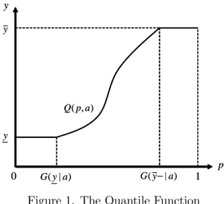
Figure 1. The Quantile Function
The interpretation is straightforward when the distribution is expressed in terms of its quantile function. This is de…ned by
Q(p; a) = inffy j G(y j a) pg; p 2 (0; 1):
Our assumptions imply that the quantile is a continuous function, although it may be only piece-wise di¤erentiable. Figure 1 gives an illustration in the (p; y) plane when both the lower and upper bound of the support have a probability mass. In the interior of the support, the quantile is de…ned
by G (Q(p; a) j a) p. When the distribution is absolutely continuous, the
Lemma 1 eG(y; a) convex in (y; a) is equivalent to R0pQ( ; a) d concave in a for all p.
In view of Lemma 1, we henceforth refer to the condition as Concavity of the Cumulative Quantile (CCQ). It is equivalent to
E (Y j a; G(Y j a) p) =
Z p 0
Q( ; a)
p d
concave in a. In words, the average return below any p-percentile is concave in a. Letting p tend to unity, the overall expected return is also concave.
In terms of the quantile function, expected utility is U (a)
Z 1 0
u(Q(p; a) a) dp: (3)
If Q(p; a) is concave in a, so is the integrand in (3) and therefore the expected utility. A concave quantile function obviously implies CCQ. The latter turns out to be su¢ cient for the concavity of the decision-maker’s problem. Proposition 1 Expected utility is concave in a if the distribution of returns satis…es CCQ.
When the distribution is absolutely continuous, G(y j a) quasiconvex in
a and y is equivalent to Q(p; a) concave in a for all p (see Jewitt 1988).
The return can then be interpreted as generated by a stochastic production function y = '(a; ") that is concave in a in each state of the world ". The CCQ condition then corresponds to the weaker requirement that marginal returns to investment are on average decreasing in bad states.
Many common probability distributions satisfy CCQ given an appropriate parameterization. To illustrate, if returns have the exponential distribution with a mean that is concave in a, the quantile function is also concave in a and therefore CCQ holds. If returns are normally distributed with mean (a) and standard deviation (a), then y = (a)+ (a)" where " is the standard normal
variable. Its quantile is Q"(p)so that
R1
0 Q"(p) dp = 0. The quantile of returns
is then Q(p; a) = (a)+ (a)Q"(p). When the standard deviation is constant, 00(a) 0implies that the quantile of returns is concave. When the standard
deviation varies with a, the quantile cannot be concave because Q"(p) varies
between minus and plus in…nity. However, because R0pQ"( ) d 0,
Z p 0 Qaa( ; a) d = 00(a) + 00(a) Z p 0 Q"( ) d 0
if the mean is a concave function and dispersion is convex. The same argu-ment also holds if " is a continuous but otherwise arbitrary random variable.
Two points need to be emphasized. First, the convexity of eG is
incon-sistent with a probability mass at the lower bound of the support, except in the particular case where the probability does not vary with a.2 Second, the same condition is required for the quasiconvexity of G to imply the concavity of the quantile in a. Indeed, the CCQ condition implies that Q(p; a) is con-cave in a for p su¢ ciently small. This is easily shown to be consistent with a probability mass at the lower bound only if the probability is constant.3
Log-Convexity of the Distribution Function (LCDF). We now
discuss a more restrictive set of conditions. By contrast with CCQ, how-ever, they are compatible with a non-constant probability mass at the lower bound of the support. The distribution of returns satis…es LCDF if ln G
is convex in a. We combine this property with the condition that the
2For instance, G(y j a) is always equal to zero. An example with a positive constant is the case of accidental losses when the probability of no accident does not depend on pre-vention expenditures, although prepre-vention a¤ects the severity of losses should an accident occur.
3To illustrate, let G(y j a) = 1 '(a) exp ( (y= (a))) where y 0 with '(a) 2 (0; 1) and (a) twice di¤erentiable and nondecreasing concave. Conditional on y > 0, the distribution of returns has the exponential density with mean (a). The quantile is Q(p; a) = 0 if '(a) 1 p and Q(p; a) = (a) ln ((1 p)='(a)) otherwise. Qaa(p; a) 0 whenever '(a) 6= 1 p. The distribution is quasiconvex but the quantile is not concave in a unless '(a) is a constant.
decision-maker’s utility function satis…es NIARA; that is, absolute risk aver-sion r(w) u00(w)=u0(w)is nonincreasing.
Proposition 2 Expected utility is concave in a if G satis…es LCDF and the
utility function satis…es NIARA.
The proof is similar to that in Abraham et al. (2011) except that we allow probability masses at the bounds of the support. LCDF is stronger than CDF (i.e., G convex in a), itself a restrictive condition as already noted. In the Appendix we show that, because of wealth e¤ects, CDF is not su¢ cient to ensure that expected utility is concave.4
LCDF has the following interpretation in terms of decreasing marginal returns. The ratio g=G is the reverse hazard rate, the probability of the realization y conditional on the outcome being no more than y. It is easily seen that ln(G(yj a)) = Z y y g( j a) G( j a)d : (4)
LCDF means that the cumulative reversed hazard rate is concave in a. When a larger expenditure increases returns in the sense of …rst-order stochastic dominance, the cumulative reversed hazard rate is increasing in a. LCDF imposes that it increases at a decreasing rate.
3
The Principal-Agent Problem
The random return facing the individual, henceforth the agent, now origi-nates from the contract designed by the principal. The observable outcome is x distributed according to F (x j a), a twice-continuously di¤erentiable dis-tribution with density f (x j a); the support is [x; x] for all a. We make the
4An example of a distribution satisfying LCDF is the function used in Rogerson (1985) to illustrate CDF, G(y j a) = (y=y)a, y 2 [0; y], a > 0.
standard assumption that the distribution satis…es the strict MLR condition, fa(x j a)=f(x j a) strictly increasing in x for all a. We also assume that the
likelihood ratio is bounded below. This precludes near-forcing contracts as in Mirrlees (1999). When the agent faces a limited liability constraint, it also allows for the possibility that the constraint is not binding in the optimal contract.5
A contract is a piece-wise di¤erentiable function y(x). This describes a deterministic scheme. In a general framework permitting nonseparable utility, Kadan et al. (2011) show that randomization is unnecessary when the principal and agent have “weakly con‡icting preferences” over rewards. The condition is trivially satis…ed in our setup.6
The agent’s expected utility is U (a; y)
Z x
x
u(y(x) a)f (xj a) dx: (5)
The agent is strictly risk averse and the principal is risk neutral. We consider
the cost to the principal of implementing some level of e¤ort ba 2 (0; a).
Equivalently, one could look for the contract that maximizes the agent’s expected utility subject to the principal’s pro…t constraint.
The agent’s participation constraint is
U (ba; y) u0; (IR)
where u0 is reservation utility. His incentive compatibility constraint is
ba 2 max
a2[0;a]U (a; y): (IC )
5We focus on the case where F is absolutely continuous in order to simplify the expo-sition. Our results also hold when F is discontinuous at x. For instance, in the insurance context, x = z where z is the accidental loss and the no-loss event has positive proba-bility.
6In a two-outcome framework with the nonseparable utility v(y; a), Arnott and Stiglitz (1988) show that a su¢ cient condition for the suboptimality of randomizing contracts is that vyya 0. In our setting, vyya= u000. Arnott and Stiglitz’condition would therefore follow from NIARA.
Payments are constrained by the bounded payment conditions
y y(x) y for all x: (BP)
The lower bound will be referred to as the agent’s limited liability constraint. The principal’s cost minimization problem, denoted P , is
min
y C(ba; y)
Z x
x
y(x)f (xj ba) dx s.t. IR, IC, and BP. (P)
The relaxed problem. The …rst-order approach replaces IC with the
necessary …rst-order condition of the agent’s problem, Ua(ba; y) = 0. In
val-idating the approach, it has been common to look at the (doubly) relaxed problem where IC is replaced by
Ua(ba; y) 0: (ICR)
We assume that the relaxed problem is nondegenerate; that is, there exists piecewise di¤erentiable contracts such that the constraints are strictly slack. Let y(x) denote a solution to the relaxed problem, henceforth problem R. Given the strict MLR condition, a contract can equivalently be written
as a function of the transformed variable l fa(x j ba)=f(x j ba). Abusing
notation, we denote this representation of the contract by y(l). De…ne
(y; ) 1 + u
00(y ba)
u0(y ba) : (6)
A solution y(l) to the relaxed problem satis…es
(y(l); ) = 8 > < > : (y; ) if + l < (y; ); + l if (y; ) + l (y; ); (y; ) if + l > (y; ); (7)
for some multipliers 0and 0satisfying the complementary slackness
condition (7) implies a constant payment, which is inconsistent with ICR.
Hence, Ua(ba; y) = 0, meaning that the solution to the relaxed problem
satis…es the …rst-order condition of the true incentive-compatibility condition IC.7
Lemma 2 Let y(l) be a solution to problem R. Then y(l) is nondecreasing.
The proof does not rely on the Lagrangian conditions (see the Appendix).8 Combined with (7), the lemma implies that the set of l values for which BP does not bind is an interval. If the lower bound binds, it does so only at realizations below some critical l0; if the upper bound binds, it does only
above some critical l1. Moreover, when BP does not bind, y(l) cannot be
constant; by Lemma 2, it is therefore strictly increasing.
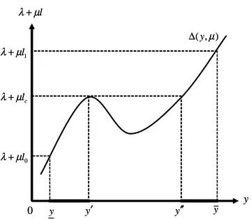
So far, nothing ensures that y(l) is continuous. One possibility is illus-trated in Figure 2. When BP does not bind, condition (7) requires that
y satis…es (y; ) = + l. Lemma 2 implies that the solution is on the
increasing portions of the curve represented in the …gure. As shown, y(l) is discontinuous at l = lc. Payments then belong to the intervals [y; y0] or
(y00; y].
Contracts satisfying the constraints of problem P also satisfy those of problem R. If a solution to the relaxed problem satis…es the true incentive-compatibility condition IC, it is therefore also a solution to the original prob-lem. Su¢ cient conditions are that the contract solving R yields a a random payment satisfying the conditions set out in Section 2. The agent’s expected utility is then concave and IC is therefore satis…ed.
7The IR constraint need not be binding, possibly because of a binding limited liability constraint. Thiele and Wambach (1999) remark that, in a nonseparable setting, IR may be slack irrespective of bounded payment constraints.
8In the separable case, v(y; a) = u(a) (e). The solution to the relaxed problem satis…es the condition (7) but with (y; ) 1=u0(y). That y(l) is increasing then follows directly from (7). This is no longer so in our problem because (y; ) as de…ned in (6) need not be increasing in y.
y l µ λ+ 0 y y y′ ) , (y µ ∆ y′′ c l µ λ+ 0 l µ λ + 1 l µ λ+ y l µ λ+ 0 y y y′ ) , (y µ ∆ y′′ c l µ λ+ 0 l µ λ + 1 l µ λ+
Figure 2. A Solution to the Relaxed Problem
Validity of the …rst-order approach. The …rst set of conditions is
in the spirit of Proposition 1. As in Jewitt (1988) for the separable setting, the conditions rely on the curvature of the contract. In Jewitt’s analysis, the conditions on the distribution of outcomes include the so-called concave
MLR condition, fa(x j a)=f(x j a) increasing and concave in x for all a,
together with one of the following two: (a) F (x j a) is quasiconvex in (x; a),
(b)RxxF ( j a) d is convex in a for all x and Rxxxf (x j a) dx is concave in a.
We will substitute the CCQ condition for (a) or (b). CCQ is weaker than (a) but implies (b). In order to apply Proposition 1 while allowing for an upward bounded payment constraint, we need the following lemma.
Lemma 3 If the random variable Z satis…es the CCQ condition, then the
variable min('(Z); k) also satis…es CCQ for any constant k and ' nonde-creasing concave and twice di¤erentiable.
In the separable setting, the conditions in Jewitt (1988) are not su¢ cient when the lower bound on payments is binding. The same is true of our second set of conditions for the nonseparable case. A binding limited liability constraint implies that the distribution of payments has a probability mass at y. Recalling section 2, this is inconsistent with CCQ. In what follows, p(w) u000(w)=u00(w)is absolute prudence.
Proposition 3 Let y(x) be a solution to problem R. Su¢ cient conditions
for y(x) to solve problem P are: (i) y(x) > y;
(ii) F satis…es the CCQ and concave MLR conditions;
(iii) p(w) 2r(w) and p0(w) min [0; (r(w) p(w))(2r(w) p(w)] for all
w2 [y a; y].
Condition (i) states that the lower bound on payments is not binding in the solution to the relaxed problem. Condition (iii), which is further dis-cussed below, implies that (y; )is convex in y whenever it is nondecreasing. Condition (ii) then implies that the random payment satis…es the CCQ con-dition, so Proposition 1 applies. See the Appendix for details. In the next subsection we discuss how both the CCQ and concave MLR conditions can be relaxed.
In condition (iii), the inequality p 2r is equivalent to 1=u0 convex in
wealth.9 This is satis…ed, for instance, if relative risk aversion is not less
than unity and is nondecreasing. Roughly speaking, the second inequality in condition (iii) states that prudence does not decrease too fast over the domain of feasible wealth levels. It su¢ ces that prudence be nondecreasing.
9This condition was used by Grossman and Hart (1983) in the separable setting to ensure that the wage is a concave function of the likelihood ratio. Jewitt (1988) imposes only that u(v(z)) be concave in z, where v(z) (u0) 1(1=z). This is equivalent to p 3r. See Conlon (2009) for a discussion.
However, noting that r0 = r(r p), the condition is also consistent with
decreasing prudence when absolute risk aversion is itself decreasing.10
To illustrate, consider the family of utility functions with constant
pru-dence, p(w) = > 0 for all w. Solving the di¤erential equation yields
u(w) = w e w where 0. When = 0, this is the CARA
util-ity function with absolute risk aversion equal to , which obviously satis…es condition (iii). When > 0, risk aversion is
r(w) =
2
+ e w
and is decreasing in wealth. The condition p(w) 2r(w) then amounts to
e w . For < , the condition is satis…ed as long as w ln ( = ) = .
Thus, it su¢ ces that the upper bound y be less than this quantity. Another class of utility functions that is easily seen to satisfy condition (iii) consists of functions with marginal utility satisfying
u0(w) = ( w) , > 0, > 0, 1, 0 w = :
For = 1, this is the quadratic utility function, hence prudence is zero. The second set of conditions is with respect to Proposition 2. As in Jewitt et al. (2008) for the separable case, the following holds under both downward and upward bounded payments constraints.
Corollary 1 Suppose that the agent’s utility function satis…es NIARA and
that F satis…es the MLR and LCDF conditions. Then the solution to R is also the solution to the original problem P.
The proof follows from the observation that, if a random variable satis-…es LCDF, so does any nondecreasing transformation. MLR together with Lemma 2 therefore imply that the distribution of payments satis…es the con-dition of Proposition 1.
Information systems. Jewitt (1988) and Conlon (2009) interpret the concave MLR condition as meaning that variations in output become “less informative” at high levels of output. Yet in many situations the outcome is a pure signal. When it satis…es the MLR condition, so does any strictly increasing transformation. Moreover, the transformed signal provides the same information. Unless the transformation is concave, properties such as CCQ and concave MLR need not be preserved. Nevertheless, if a contract conditioning on the original signal solves the principal’s problem, a suitably speci…ed contract conditioning on the transformed signal will do the same. For validating the …rst-order approach, one should therefore also look for properties that are robust to arbitrary strictly increasing transformations of the signal. Such properties will be referred to as informational because they characterize the underlying information system.
LCDF is preserved under increasing transformations. The condition on the signal distribution in Corollary 1 is therefore informational. We look for informational properties to substitute for the non informational properties in condition (ii) of Proposition 3.
De…nition 1 Let X be distributed according to F (x j a) with associated
density f (x j a) satisfying the MLR condition. F satis…es Likelihood-CCQ if, for all a0, the distribution of f
a(X j a0)=f (X j a0) satis…es CCQ.
The random variable fa(X j a0)=f (X j a0) will be referred to as the
likelihood ratio transform at a0. Note that its distribution depends on the agent’s e¤ort a.
Corollary 2 If X satis…es the MLR and Likelihood-CCQ conditions, so does
any strictly increasing transformation. Moreover, condition (ii) in Proposi-tion 3 can be replaced by: F satis…es the MLR and Likelihood-CCQ condi-tions.
The second claim follows from the fact that the agent’s wage will then satisfy CCQ when the other conditions in Proposition 3 hold. The …rst claim states that Likelihood-CCQ is an informational property. To see this, let
Z '(X)where ' is strictly increasing. The distribution of the transformed
signal is F (' 1(z) j a). Its likelihood ratio transform at a0 is the random variable
fa(' 1(Z)j a0)=f (' 1(Z)j a0):
Clearly this has the same distribution as the likelihood ratio transform at a0
of the original signal.
The condition means that the agent faces decreasing marginal returns to e¤ort in the generation of “favorable information”. If X satis…es both the CCQ and concave MLR conditions, then it satis…es Likelihood-CCQ. Any strictly increasing transformation will then also satisfy Likelihood-CCQ, although the transformed signal need not satisfy CCQ or the concave MLR condition. To illustrate, suppose the signal has the Weibull distribution
F (x j a) = 1 exp (x=a )k, where and k are positive parameters and
x 0. The signal satis…es CCQ if 1 and the concave MLR condition if
k 1. Likelihood-CCQ is the weaker condition k 1.
4
Concluding remarks
There will obviously be cases where the …rst-order approach is valid even though the above su¢ cient conditions are not met; that is, the solution to the relaxed problem is nevertheless the solution to the true problem. Lemma 2 shows that the payment to the agent is then increasing with “more favorable” information, as in the standard model where utility is additively separable in income and e¤ort. The principal’s cost is then increasing in the e¤ort level that is to be implemented, an important property of the …rst-order approach. The CCQ condition or the weaker Likelihood-CCQ may be appealing in the additively separable case as well. When the agent’s limited liability
condition is not binding, Likelihood-CCQ ensures the validity of the …rst-order approach under Jewitt’s (1988) conditions with respect to the agent’s utility of income function. Because Proposition 3 speci…es more restrictive conditions, they are also su¢ cient in the mixed case where e¤ort entails both psychological disutility and money expenditure; that is, the agent’s utility
function is u(y c(a)) (a) where the money cost and the disutility are
both increasing convex functions.
Appendix
Non su¢ ciency of CDF. We give an example showing that U0(a) = 0
characterizes a global minimum even though the distribution of returns sat-is…es CDF. The decision-maker’s utility function is CARA with u(w) = exp( rw). The return is the function y(X) of the random variable X
with support [0; 1] and cdf F (x j a) = x (x) (a), where (x) = x(1 x),
(a) = (1 k)a + k ln(1 + a); k 2 [0; 1]. The cdf belongs to a family of
distributions satisfying both the MLR and CDF conditions; see LiCalzi and Spaeter 2003. Because these properties are robust to arbitrary increasing transformations, the returns satisfy MLR if y( ) is an increasing function. Let r = k = 0:1 and y(X) = bX. We consider U (a) for a 2 [0; 1]. Figure A1 depicts the graph for b = 6; the curve is convex with a maximum at
a = 1and a global minimum at a = 0:285. In Figure A2, b = 5:85; the curve
is again convex but with a maximum at a = 0 and a global minimum at a = 0:769.
0.2 0.4 0.6 0.8 1 -0.7519 -0.7518 -0.7517 -0.7516 -0.7515 ) (a U a 0.2 0.4 0.6 0.8 1 -0.7519 -0.7518 -0.7517 -0.7516 -0.7515 ) (a U a Figure A1: b = 6 0.2 0.4 0.6 0.8 1 -0.7582 -0.7578 -0.7576 -0.7574 -0.7572 ) (a U a 0.2 0.4 0.6 0.8 1 -0.7582 -0.7578 -0.7576 -0.7574 -0.7572 ) (a U a Figure A2: b = 5:85
Proof of Lemma 1. De…ne
e Q(p; a) Z p 0 Q( ; a) d and eG(y; a) Z y y G(zj a) dz:
Because the quantile is the convex conjugate of the cumulative distribution, for all p 2 (0; 1) we have
e
Q(p; a) = pQ(p; a) G(Q(p; a); a)e (8)
py G(y; a)e for all y 2 [y; y]: (9)
We …rst show that the convexity of eG(y; a)implies the concavity of eQ(p; a)
in a. Let a = a0+ (1 )a00 and y = y0+ (1 )y00 where 2 (0; 1). From
(8) and (9),
e
implies e
Q(p; a) (py0 G(ye 0; a0)) + (1 )(py00 G(ye 0; a00)): Therefore, setting y0 = Q(p; a0) and y00 = Q(p; a00)yields
e
Q(p; a) Q(p; ae 0) + (1 ) eQ(p; a00):
Next we show that eQ(p; a) concave in a implies the convexity of eG(y; a). From (8) and (9),
e
G(y0; a0) + (1 ) eG(y00; a00) py ( eQ(p; a0) + (1 ) eQ(p; a00)) py Q(p; a);e
where the second inequality follows from the concavity of eQ(p; a)in a. Setting p = G(y j a), the right-hand side in the string of inequalities equals
G(y j a)y Q(G(ye j a); a) = eG(y; a); implying that eG(y; a) is convex. QED
Proof of Proposition 1. We …rst prove a preliminary result.
Step 1. For p 2 [0; 1] and a 2 [0; a], let w(p; a) be a continuous function, nondecreasing in p and piecewise di¤erentiable with respect to p and a. De…ne
e w(p; a) Z p 0 w( ; a) d and U (p; a) Z p 0 u(w( ; a)) d .
We show that U (p; a) is concave in a if w(p; a)e is concave in a. Observe
that w(p; a)e and U (p; a) are di¤erentiable with respect to a. Recall that u is increasing concave and twice-continuously di¤erentiable. The concavity implies that, for any a and a ,
u(w( ; a)) u(w( ; a )) u0(w( ; a))(w( ; a) w( ; a ))
and therefore
U (p; a) U (p; a ) Z p
0
Denote by wp+(p; a) the right-hand derivative of w(p; a) with respect to p.
Integrating by parts, the right-hand side of (10) equals u0(w(p; a)) (w(p; a)e w(p; a ))e
Z p 0
u00(w( ; a))wp+( ; a)(w( ; a)e w( ; a )) d :e
Substituting in (10) and noting that the concavity of w(p; a)e implies e w( ; a) w( ; a )e wea( ; a)(a a ), we obtain U (p; a) U (p; a ) (a a ) u0(w(p; a))wea(p; a) Z p 0 u00(w( ; a))wp+( ; a)wea( ; a) d :
Integrating by parts the expression in the parentheses,
U (p; a) U (p; a ) (a a )
Z p 0
u0(w( ; a))wa( ; a) d = (a a )Ua(p; a):
Hence U (p; a) is concave in a for all p.
Step 2. We now turn to the claim in the proposition. Write the expected utility using the quantile formulation (3). By Lemma 1, CCQ implies that Rp
0(Q( ; a) a) d is concave in a. Letting w(p; a) Q(p; a) aand applying
Step 1 then completes the proof. QED
Proof of Proposition 2. We start with a preliminary result. Let H(y; a) be
a positive continuous function, di¤erentiable and increasing in y 2 (y0; y1)
(y; y) and log-convex in a. De…ne
U (a; y0; y1; H) u(y0 a)H(y0; a) + u(y1 a)(1 H(y1; a))
+ Z y1
y0
Integrating by parts,
U (a; y0; y1; H) = u(y1 a)
Z y1
y0
u0(y a)H(y; a) dy: (11)
When r(w) is nonincreasing, u0(y a) is log-convex in a. It follows that
u0(y a)H(y; a) is also log-convex in a, hence the integral in (11) is convex,
implying that U (a; y0; y1; H)is concave.
Now consider the expected utility in (2) and assume NIARA. We discuss the cases where the support of G is either unbounded at both ends or bounded
at both ends; the argument for the mixed cases is similar. When y = 1
and y = +1,
U (a) = lim
y1!+1
y0! 1
U (a; y0; y1; G):
Therefore, if G is log-convex in a, U (a) is concave. For the case of a bounded support, let y0 = y and y1 = y with
H(y; a) = G(y j a) +
Z y y
g(zj a) dz; y 2 [y; y]:
Hence H(y; a) = G(y j a) for y < y and H(y; a) G(y j a), where the
inequality is strict if there is a jump at the upper bound. It follows that U (a) = U (a; y; y; H). If G is log-convex in a, so is H and therefore U (a) is concave. QED
Proof of Lemma 2. If y(x) solves problem R, the agent’s expected utility
is
U (ba; y) =
Z x
x
u(y(x) ba)f(x j ba) dx u0
and marginal expected utility satis…es Ua(ba; y) =
Z x
x
u(y(x) ba)fa(xj ba) dx
Z x
x
u0(y(x) ba)f(x j ba) dx = 0: The cost to the principal is
C(ba; y)
Z x
x
Let QX(p; a)be the quantile of the signal. De…ne
l(p) fa(QX(p;ba) j a)=f(QX(p;ba) j ba):
Strict MLR implies that l(p) is strictly increasing. Let w(p) y(l(p)). The
above expressions can then be rewritten as U (ba; w) = Z 1 0 u(w(p) ba) dp; Ua(ba; w) = Z 1 0 u(w(p) ba)l(p) dp Z 1 0 u0(w(p) ba) dp: (12) C(ba; w) Z 1 0 w(p) dp:
If y(l) is not nondecreasing, the same is true of w(p). Hence, there exists two disjoint intervals [p0; p0+ ] [0; 1] and [p00; p00+ ] [0; 1], p0+ < p00,
such that w(p) > w(p)e for all p 2 [p0; p0 + ] and pe2 [p00; p00+ ]. Consider the contract b w(p) = 8 > < > : w(p)if p =2 [p0; p0 + ][ [p00; p00+ ]; w(p00 p0+ p) if p 2 [p0; p0 + ]; w(p0 p00+ p) if p 2 [p00; p00+ ]:
For any function ', Z 1 0 '(w(p)) dp =b Z 1 0 '(w(p)) dp: Indeed Z p0+ p0 '(w(p)) dp =b Z 0 '(w(pb 0+ )) d = Z 0 '(w(p00+ )) d = Z p00+ p00 '(w(p)) dp, Z p00+ p00 '(w(p)) dp =b Z 0 '(w(pb 00+ )) d = Z 0 '(w(p00+ )) d = Z p0+ p0 '(w(p)) dp.
Expected utility and the principal’s cost are therefore unchanged under b
w(p). The same is true of the second term on the right-hand side of (12. However, Ua(ba; bw) > Ua(ba; w) because
Z 1 0 u(w(p)b ba)l(p) dp > Z 1 0 u(w(p) ba)l(p) dp;
To see this, u(p) = u(w(p) ba), bu(p) = u( bw(p) ba) and observe that Z p0+ p0 bu(p)l(p) dp = Z 0 bu(p0+ )l(p0+ ) d = Z 0 u(p00+ )l(p0+ ) d ; Z p00+ p00 bu(p)l(p) dp = Z 0 bu(p00+ )l(p00 + ) d = Z 0 u(p0+ )l(p00+ ) d : Therefore Z 1 0 bu(p)l(p) dp Z 1 0 u(p)l(p) dp = Z 0 (u(p00+ ) u(p0 + )) l(p0+ ) l(p00+ ) d :
On the right-hand side, both factors in the integrand are negative, so the expression is positive.
Finally, Ua(ba; bw) > Ua(ba; w) implies that w(p) cannot be a solution to
problem R. Let "(p) w(p)b C(ba; w) so that R01"(p) dp = 0. Consider the contracts
e
w(p) C(ba; w) + "(p), 2 [0; 1]:
All these contracts yield the same costs to the principal when the agent’s e¤ort isba. Denote expected utility and marginal expected utility by U(ba; ) and Ua(ba; ) respectively. For all < 1, U (ba; ) > U(ba; 1) = u0 because is
a mean preserving decrease in risk. From the previous argument Ua(ba; 1) > 0.
Therefore , by continuity, for some < 1 both the IR and ICR constraints
are slack. For positive but small enough, they will remain slack under the
contract
e
which costs less than C(ba; w). QED
Proof of Lemma 3. Denote by QZ(p; a) the quantile function of Z. The
quantile of '(Z) is then Q'(p; a) '(QZ(p; a)). First, observe that the
dis-tribution of '(Z) satis…es CCQ when Z does. To see this, use the argument
in Step 1 of Proposition 2 with QZ(p; a) w(p; a)and ' u. Next we that
the distribution of min('(Z); k) also satis…es CCQ. Its quantile function is Qm(p; a) min('(QZ(p; a)); k). Obviously
e Qm(p; a) Z p 0 Qm(p; a) d Qe'(p; a) Z p 0 Q'(p; a) d :
It su¢ ces to show that the concavity of eQ'(p; a)in a implies that of eQm(p; a).
Let p(a)b be the the solution to Q'(bp(a); a) = k. When p p(a),b 2 [0; 1]
and a = a0+ (1 )a00 imply e Qm(p; a) = Qe'(p; a) e Q'(p; a0) + (1 ) eQ'(p; a00) e Qm(p; a0) + (1 ) eQm(p; a00): (13) For p >p(a)b , e Qm(p; a) = eQ'(p(a); a) + (pb p(a))k:b Observe that (p p(a))kb Z p b p(a) Qm( ; a0) d + (1 ) Z p b p(a) Qm( ; a00) d :
Combining with (13) yields e Qm(p; a) = Qe'(p(a); a) + (pb p(a))kb e Qm(p(a); ab 0) + (1 ) eQm(p(a); ab 00) + Z p b p(a) Qm( ; a0)d + (1 ) Z p b p(a) Qm( ; a00)d e Qm(p; a0) + (1 ) eQm(p; a00);
which completes the proof. QED
Proof of Proposition 3. Write the contract solving R as y(l), l 2 [l; l]
where l = fa(xj ba)=f(x j ba), l = fa(xj ba)=f(x j ba).
Step 1. Suppose that y(l) is continuous and the BP constraints are not binding for l 2 [l0; l1] [l; l]. By Lemma 2 and because (y(l); ) = + l,
it follows that y(l) is strictly increasing in that interval. Hence, y(y; ) 0
for y 2 [y(l0); y(l1)] with strict inequality almost everywhere. We show that
condition (iii) then implies yy(y; ) 0 for y 2 (y(l0); y(l1)). For y in this
interval, y(y; ) = u000u0 u00(1 + u00) (u0)2 0: (14) Then yy(y; ) = u0000u0 u000(1 + u00) (u0)2 2u 00 u000u0 u00(1 + u00) (u0)3 = u 0000u0 u000(1 + u00) (u0)2 + 2 u00 u0 y(y; ): (15) Note that p0 = (u000=u00)2 (u0000=u00). Hence u0000 (u000)2=u00 is equivalent to
p0 0. Under this condition,
yy(y; ) (u000)2 u00 u 0 u000(1 + u00) (u0)2 + 2 u00 u0 y(y; ) = (2r p) y(y; ):
Hence, p 2rand p0 0are su¢ cient for
yy 0whenever y 0. Noting
that r0 = r(r p), di¤erentiating (14) once more is easily seen to yield yy(y; ) =
r (2r p)
u0 r [(r p)(2r p) p
0] :
Hence, p 2r and p0 r0(2 p=r) are also su¢ cient for
yy 0.
Step 2. Condition (i) implies that y(l) is an interior solution solving (y; ) = + lfor all l 2 [l; l1]for some l1 2 (l; l]. Without loss of generality,
we can discard the possibility that y(l) is discontinuous at l (otherwise it is an isolated point). Thus, y(l) is continuous in a right neighborhood of l and Step 1 therefore applies; that is, for y(l) in a right neighborhood of l, y(l) is
strictly increasing, y(y(l); ) 0 with strict inequality almost everywhere
and yy(y(l); ) 0 . But this then implies that the same is true for all
y > y(l). Hence the contract satis…es
y(l) = min 1( + l); y ;
where 1is the inverse of (y; )with respect to its …rst argument. Because
1 is increasing concave and applying Lemma 3, the distribution function
of the payment then satis…es CCQ if the distribution of fa(X j ba)=f(X j ba)
does. The latter, again using Lemma 3, is ensured by condition (ii). QED
References
Abraham, A., Koehne, S. and N. Pavoni (2011), “On the First-Order Ap-proach in Principal-Agent Models with Hidden Borrowing and Lend-ing.” Journal of Economic Theory 146, 1331-1361.
Alvi, E. (1997), “First-Order Approach to Principal-Agent Problems: A Generalization.”Geneva Papers on Risk and Insurance Theory 22, 59-65.
Arnott, R. and J.E. Stiglitz (1988), “Randomization with Asymmetric In-formation.” RAND Journal of Economics 19, 344-362.
Carlier, G. and R.A Dana (2005), “Existence and Monotonicity of Solutions to Moral Hazard Problems.” Journal of Mathematical Economics 41, 826-843.
Conlon, J.R. (2009), “Two New Conditions Supporting the First-Order Ap-proach To Multisignal Principal-Agent Problems.” Econometrica 77, 249-278.
Eeckhoudt, L. and Ch. Gollier (2005), “The Impact of Prudence on Optimal Prevention.” Economic Theory 26, 989-994.
Grossman, S. and O. Hart (1983), “An Analysis of the Principal-Agent Problem.” Econometrica 51, 7–45.
Holmstrom, B. and P. Milgrom (1987), “Aggregation and Linearity in the Provision of Intertemporal Incentives.” Econometrica 55, 303-328. Jewitt, I. (1988), “Justifying the First-Order Approach to Principal-Agent
Problems.” Econometrica 51, 1177-1190.
Jewitt, I., O. Kadan, J.M. Swinkels (2008), “Moral Hazard with Bounded Payments.” Journal of Economic Theory 143, 59-82.
Jullien, B., R. Salanié and F. Salanié (1998), “Should More Risk-Averse Agents Exert More E¤ort?”Geneva Papers on Risk and Insurance The-ory 24, 19-28.
Kadan, O., Ph.J. Reny and J.M. Swinkels (2011), “Existence of Optimal Contracts in the Moral Hazard Problem.”MFI working paper no 2011-02.
Kawasaki, S. and J. McMillan (1987), “The Design of Contracts: Evidence from Japanese Subcontracting.” Journal of the Japanese and Interna-tional Economies 1, 327-349.
LiCalzi, M. and S. Spaeter (2003), “Distributions for the First-Order Ap-proach to Principal-Agent Problems.” Economic Theory 21, 167-173. McAfee, P. and J. McMillan (1986), “Bidding for Contracts: A
Principal-Agent Analysis.” RAND Journal of Economics 17, 326-328.
Martimort, D. and J. Pouyet (2008), “To Build or Not to Build: Normative and Positive Theories of Public-Private Partnerships.” International Journal of Industrial Organization 26, 393-411.
Meyer, D.J. and J. Meyer (2011), “A Diamond-Stiglitz Approach to the Demand for Self-Protection.” Journal of Risk and Uncertainty 42, 45-60.
Mirrlees, J. (1999) “The Theory of Moral Hazard and Unobservable Behav-ior: Part I.” Review of Economic Studies 66, 3-21.
Rogerson, W.P. (1985), “The First-Order Approach to Principal-Agent Prob-lems.” Econometrica 53, 1375–67.
Sinclair-Desgagné, B. (1994), “The First-Order Approach to Multidimen-sional Principal-Agent Problems.” Econometrica 62, 459-465.
Thiele, H. and A. Wambach (1999), “Wealth E¤ects in the Principal Agent Model.” Journal of Economic Theory 89, 247-260.