Any correspondence concerning this service should be sent to the repository administrator:
staff-oatao@inp-toulouse.fr
This is an author-deposited version published in:
http://oatao.univ-toulouse.fr/
Eprints ID: 9028
To cite this version:
Devaurs, Didier and Siméon, Thierry and Cortés Mastral, Juan Enhancing the
Transition-based RRT to deal with complex cost spaces. (2013) In: IEEE
International Conference on Robotics and Automation, ICRA '13, 6-10 May
2013, Karlsruhe, Germany.
O
pen
A
rchive
T
oulouse
A
rchive
O
uverte (
OATAO
)
OATAO is an open access repository that collects the work of Toulouse researchers and
makes it freely available over the web where possible.
Enhancing the Transition-based RRT to Deal with Complex Cost Spaces
Didier Devaurs, Thierry Sim´eon and Juan Cort´es
Abstract— The Transition-based RRT (T-RRT) algorithm en-ables to solve motion planning problems involving configuration spaces over which cost functions are defined, or cost spaces for short. T-RRT has been successfully applied to diverse problems in robotics and structural biology. In this paper, we aim at enhancing T-RRT to solve ever more difficult problems involving larger and more complex cost spaces. We compare several variants of T-RRT by evaluating them on various motion planning problems involving different types of cost functions and different levels of geometrical complexity. First, we explain why applying as such classical extensions of RRT to T-RRT is not helpful, both in a mono-directional and in a bidirectional context. Then, we propose an efficient Bidirectional T-RRT, based on a bidirectional scheme tailored to cost spaces. Finally, we illustrate the new possibilities offered by the Bidirectional T-RRT on an industrial inspection problem.
I. INTRODUCTION
Sampling-based motion planning has traditionally aimed at finding feasible paths, i.e. collision-free paths, to solve com-plex planning problems in high-dimensional spaces, without considering the quality of the produced paths. In many application fields, however, it is important to compute good-quality paths w.r.t. a given cost criterion. If a feasible solution path is found quickly, it is possible to allocate additional computation time to improve the solution. Nevertheless, the smoothing methods classically used during such post-processing phase only allow to locally improve the path. For better results, the cost criterion must be taken into account during the space exploration itself.
The first approaches dealing with sampling-based motion planning on cost spaces were based on the Rapidly-exploring Random Tree (RRT) algorithm [1]. Unfortunately, they were all focused on specific applications in the area of 2D robot navigation [2]–[7], and some of them were evaluated only on configuration spaces involving very coarse-grained, discrete cost functions [2]–[4]. More importantly, all these methods suffer from different practical drawbacks [8]. For example, some of them rely on the estimated cost-to-goal, which tends to bias the search straight toward the goal at the expense of better-quality paths [2]–[4]. Also, the threshold-based method presented in [5], [6] suffers from the non-decreasing nature of its threshold and from its high sensitivity to the increase rate of the threshold [8].
Apart from grid-based methods, such as A*, the first general approach to cost-space planning was the Transition-based RRT (T-RRT) algorithm [8], that combines the
ex-All authors are with CNRS, LAAS, 7 avenue du colonel Roche, F-31400 Toulouse, France and Univ de Toulouse, LAAS, F-31400 Toulouse, France (e-mails: devaurs@laas.fr, nic@laas.fr, jcortes@laas.fr)
This work has been partially supported by the European Community under Contract ICT 287617 “ARCAS”.
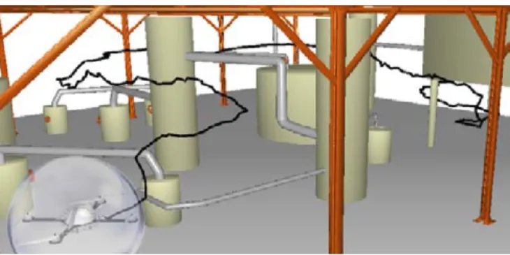
Fig. 1. Path produced by the Bidirectional T-RRT for a quadrotor flying in a dense industrial environment.
ploratory strength of RRT with a stochastic optimization mechanism. T-RRT has been successfully applied to various robot path-planning problems [8]–[11] (some even involving human–robot interactions [9]) as well as structural biology problems [11], [12]. When compared to previous meth-ods [2], [5], T-RRT produced better-quality paths [8]. But, it has been shown that RRT (and thus T-RRT) cannot converge toward an optimal solution [13]. That is why a variant of RRT offering asymptotic-optimality guarantees, namely RRT*, was developed [13]. However, it has been observed that RRT* may converge slowly in high-dimensional spaces, and that T-RRT may provide a reasonably good solution faster [11].
In this paper, we discuss extensions to T-RRT aimed at improving its performance. We first present the details of the T-RRT algorithm (Section II) and the motion planning problems used in our evaluation (Section III). T-RRT being based on the basic Extend RRT, one may think that the exten-sions improving RRT are also beneficial to T-RRT. We show that this is not the case for the Goal-biased and the Connect variants (Section IV). Since the Bidirectional scheme pro-posed for RRT in [1] does not improve performance either, we propose a tailored and efficient Bidirectional T-RRT, and then compare it to RRT* (Section V). Finally, we present an industrial inspection problem that only the Bidirectional T-RRT can solve efficiently (Section VI, Fig. 1).
II. TRANSITION-BASEDRRT
T-RRT extends RRT by integrating a stochastic transition test enabling it to bias the exploration toward low-cost regions of the configuration space [8]. This transition test is based on the Metropolis criterion typically used in Monte Carlo optimization methods [14]. These techniques aim at finding global minima in complex spaces and involve ran-domness as a means to avoid being trapped in local minima. Similarly to these methods, T-RRT uses a transition test to
Algorithm 1: Transition-based RRT
input : the configuration spaceC ; the cost function c :C → R+; the root qinit; the goal qgoal
output: the tree T
1 T ← initTree(qinit)
2 while not stopCondition(T , qgoal) do
3 qrand← sampleRandomConfiguration(C)
4 qnear← findNearestNeighbor(T , qrand)
5 if refinementControl(T , qnear,qrand) then
6 qnew← extend(qnear, qrand)
7 if qnew6= null
8 and transitionTest(T , c(qnear), c(qnew)) then
9 addNewNodeAndEdge(T , qnear, qnew)
Algorithm 2: transitionTest (T , ci, cj)
input : the cost threshold cmax; the current temperature T ;
the temperature increase rate Trate
output: true if the transition is accepted, and false otherwise
1 if cj> cmax then return False
2 if cj≤ ci then return True
3 if exp(−(cj− ci) / T ) > 0.5 then
4 T ← T / 2(cj−ci) / (0.1 · costRange(T )); return True
5 else
6 T ← T · 2Trate ; return False
accept or reject a candidate state, based on the cost variation associated with the local motion. The pseudo-code of T-RRT (shown in Algorithm 1) is similar to that of the basic Extend RRT [1], with the addition of the transitionTest and refinementControl functions.
The transitionTest presented in Algorithm 2 is an improved version of the one proposed in [8]. It is used to evaluate the transition from qnear to qnew based on their
respective costs. Three cases are possible: 1) A new config-uration whose cost is higher than the threshold value cmax1
is automatically rejected. 2) A transition corresponding to a downhill move is always accepted. 3) Uphill transitions are accepted or rejected based on a probability that decreases exponentially with the cost variation cj − ci, similarly to
the Metropolis criterion. In that case, the level of difficulty of the transition test is controlled by the adaptive parameter T , called temperature only by analogy to statistical physics. Low temperatures limit the expansion to gentle slopes, and high temperatures enable to climb steep slopes. In T-RRT, the temperature is dynamically tuned during the search process: 1) After each accepted uphill transition, T is decreased to avoid over-exploring high-cost regions. 2) After each rejected uphill transition, T is increased to facilitate exploration and avoid being trapped in a local minimum.
The adaptive tuning of the temperature ensures a given success rate for uphill transitions, but can also produce an unwanted side-effect: T may be reduced by the acceptation of new states close to states already contained in the tree, whereas increasing T may be required to go over a local cost
1A value can be provided for c
maxwhen high-cost regions of the space
have to be forbidden.
Algorithm 3: refinementControl (T , qnear, qrand)
input : the extension step-size δ ; the refinement ratio ρ output: true if refinement is not too high, and false otherwise
1 if distance(qnear, qrand) < δ
2 and nbRefinementNodes(T ) > ρ · nbNodes(T ) then 3 return False
4 return True
barrier and explore new regions of the space. Accepting such states only contributes to refining the exploration of low-cost regions already reached by the tree. The objective of the refinementControlfunction (shown in Algorithm 3) is to limit this refinement and facilitate tree expansion toward unexplored regions. The idea is to reject an expansion that would lead to more refinement if the number of refinement nodes already present in the tree is greater than a certain ratio ρ of the total number of nodes, a refinement node being defined as a node whose distance to its parent is less than the extension step-size δ. Another benefit of the refinement control is to limit the number of nodes in the tree, and thus to reduce the computational cost of the nearest-neighbor search. Following [8], we set ρ = 0.1.
Compared to the version presented in [8], the transition test shown in Algorithm 2 includes three improvements. (1) The first one appears at line 3. We have replaced the boolean expression rand(0, 1) < exp(−(cj − ci) / T ) by
exp(−(cj− ci) / T ) > p with p = 0.5 to better control the
stochastic aspect of the Metropolis test. Using rand(0, 1) instead of a fixed probability p has the following detri-mental consequence: steep uphill moves can be accepted if rand(0, 1) is close to 1, and gentle uphill moves can be rejected if rand(0, 1) is close to 0. We have varied the value of p and observed that this change has no impact on the exploration, except if p is close to 1. In fact, the adaptive nature of the temperature compensates any change in p: if p is lowered, the temperature simply reaches higher values. (2) The second improvement appears at line 6. It consists of progressively increasing the temperature after each rejection, instead of increasing it by performing a single larger jump after a given number of consecutive rejections. For that, after each rejected uphill transition, T is multiplied by 2Trate, where T
rate ∈ ]0, 1] is the temperature increase
rate. (3) The third improvement appears at line 4 and is borrowed from [11]. It consists of providing an implicit refinement control mechanism by making the temperature decrease dependent on the cost variation associated with an accepted uphill transition. For that, T is divided by 2(cj−ci) / (0.1 · costRange(T )), where costRange(T ) is the
cost difference between the highest-cost configuration and the lowest-cost configuration of the tree. After evaluation, it appears that all these modifications improve the performance of T-RRT: running times are significantly reduced without incurring any loss in path quality.
In the space where configurations whose cost is greater than cmax are regarded as part of the obstacle regions,
Fig. 2. Search tree built by T-RRT on the Mountains problem. On this 2D cost-space, the cost is the elevation.
Fig. 3. Path computed by T-RRT on the Stones problem. The cost is the inverse of the distance between the 2-DoF disk and the obstacles.
Fig. 4. Trace of a path computed by T-RRT on the Manipulator problem. A 6-DoF manipulator arm has to get a stick through a hole while maximizing clearance (i.e. the distance to the obstacles).
Fig. 5. Path computed by T-RRT on the Inspection problem. The 6-DoF manipulator arm holds a sensor (the red sphere) that has to follow the car engine as close as possible.
of the temperature allows T-RRT to automatically balance its bias toward low-cost regions with the Voronoi bias of RRT. The Trate parameter determines a trade-off between
low computation time and high quality of the produced paths: A value not too small (e.g. 0.1) leads to a greedy search, and a lower value (e.g. 0.01) enables to produce better-quality paths. We will use only these two values for Trate. Also,
following [8], we initialize T to 10−6.
III. PLANNINGPROBLEMS ANDEVALUATIONSETTINGS
We use four planning problems to evaluate the perfor-mance of the T-RRT variants. The examples differ in terms of geometrical complexity, configuration-space dimensionality and cost-function type. The Mountains problem is the 2D cost-space illustrated by Fig. 2, in which the cost is the elevation. The Stones problem (presented in Fig. 3) is a 2-degrees-of-freedom (DoF) problem in which a disk goes across a space cluttered with rectangular-shaped stones. The objective being to maximize clearance, the cost function is the inverse of the distance between the disk and the obstacles. The Manipulator problem (illustrated in Fig. 4) involves a 6-DoF manipulator arm that has to get a stick through a hole while maximizing clearance. Therefore, the cost function is the inverse of the distance between the stick and the obstacles. In the Inspection problem (shown in Fig. 5) the same arm holds a sensor with a spherical extremity used to inspect a car engine. The objective being to keep the sensor as close as possible to the engine surface, the cost function is the distance (in millimeters) between the sphere and the engine. We set cmax= 100 for the Inspection problem (due
to the sensor’s range) and cmax= ∞ for the others.
All the algorithms are implemented within the motion planning platform Move3D [15]. To fairly assess the benefit of each T-RRT variant, no smoothing is performed on the solution paths. On a given problem, we evaluate each algorithm on the basis of the running time t (in seconds), the number of expansion attempts X, the number of nodes N in the produced tree, and various quality criteria applied to the extracted path: the average cost avgC, the maximal cost maxC, the mechanical work M W , and the integral of the cost IC. The mechanical work of a path is the sum of the positive cost variations along this path [8]. For all variables, we give values averaged over 100 runs.
IV. MONO-DIRECTIONALVARIANTS OFT-RRT Compared to the Extend RRT, several classical RRT exten-sions are known to improve performance [1]. For example, the Goal-biased RRT may converge faster to the goal. Also, with the Connect RRT, the search tree generally grows faster. However, when it comes to T-RRT, improving performance means not only reducing running time, but also increasing path quality. Thus, one may wonder whether applying these modifications of RRT to T-RRT is beneficial.
Goal-biased T-RRT: In the same way as it is done for RRT, implementing the Goal-biased T-RRT consists of modifying the sampleRandomConfiguration function (line 3 in Algorithm 1) so that it returns qgoal with a
prob-ability goalBias. The results of the evaluation of the Goal-biased T-RRT (with goalBias = 0.01 and 0.1) are shown in Table I. Using the Goal-biased T-RRT reduces running time on all examples. However, when goalBias = 0.01, path quality improves on all problems if Trate = 0.1, but
TABLE I
EVALUATION,ON FOUR PROBLEMS,OF SEVERAL VARIANTS(V)OFT-RRT: (1) Extend T-RRT, (2) Goal-biased T-RRTWITHgoalBias = 0.01, (3) Goal-biased T-RRTWITHgoalBias = 0.1, (4) Connect T-RRT, (5) Bidirectional T-RRT. ALL VALUES ARE AVERAGED OVER100RUNS.
Trate= 0.1 Trate= 0.01
V avgC maxC M W IC t (s) N X avgC maxC M W IC t (s) N X
Mountains 1 17.4 24.8 29.3 3,230 2.2 1660 6260 16.7 22.8 26.5 3,780 2.7 1150 16,400 2 17.4 24.6 28.6 3,150 0.4 778 2280 16.7 22.8 26.2 3,800 1.6 885 12,600 3 17.7 25.7 28.6 3,030 0.1 433 1400 16.7 22.7 25.2 3,630 1.3 812 11,900 4 16.4 23.2 31.2 3,780 0.4 633 2530 16.5 22.8 29.2 4,270 1.4 749 14,700 5 17.7 23.9 30.5 3,300 0.1 282 982 16.7 22.8 27.2 3,700 0.9 861 11,700 Stones 1 31.7 63.9 159 32,200 0.6 652 4080 29.5 58.1 117 28,900 5.2 711 36,000 2 31.7 63.6 152 31,200 0.5 594 3520 29.6 58.2 115 28,400 5 702 35,600 3 32.2 67.5 159 31,200 0.3 512 2910 29.8 58 111 27,600 4.7 683 34,900 4 31.5 61.4 130 33,300 0.3 399 3170 30.8 58.9 104 31,500 4.6 597 39,000 5 31.5 63.5 146 31,300 0.1 251 1790 28.6 57.2 107 28,200 1.6 548 23,400 Manipulator 1 6.3 8 8 10,200 2.1 776 7130 5.8 6.6 3.8 9,110 6.9 709 26,400 2 6.1 7.5 4.4 8,310 0.3 201 2060 5.8 6.6 2.5 7,590 0.8 119 6,820 3 6.2 7.6 3.3 7,420 0.1 92 921 5.8 6.7 2.3 7,190 0.6 89 5,640 4 5.9 7.9 8.2 11,600 1 492 3910 5.5 7.2 5.3 10,600 2.9 415 15,300 5 6 7.6 3.5 7,910 0.1 101 1170 5.7 6.7 2.3 7,710 0.8 112 7,410 Inspection 1 24.1 80.9 379 89,000 11.3 321 2720 1.7 10.9 88.9 6,260 78.4 288 23,600 2 21.5 72.6 356 77,800 10.7 293 2520 1.8 11 91.3 6,580 78.2 293 23,500 3 19.1 73.3 324 65,900 9.9 270 2340 1.6 9.9 87.4 5,870 77.5 274 23,300 4 12.3 49.9 236 45,000 9.8 146 2190 1.8 12.6 78.3 6,420 64 202 20,600 5 21.6 74.5 332 75,200 8.7 254 2530 1.6 7.5 87.2 5,750 69 304 25,200
not if Trate= 0.01. On the contrary, when goalBias = 0.1,
path quality globally improves if Trate = 0.01, but not if
Trate = 0.1, especially on 2-DoF problems. Therefore, the
Goal-biased T-RRT lacks robustness.
Connect T-RRT: Contrary to the Connect RRT, the Connect T-RRT can be implemented in various ways, due to the presence of the transition test. The simplest way consists of iterating the extend and transitionTest functions until qrand or an obstacle is reached (without
adding the intermediate states to the tree). When compared to other variants (delaying temperature tuning, or limiting uphill transitions), this implementation yields the best results, which are reported in Table I. Using the Connect T-RRT reduces running time, but does not always increase path quality, especially if Trate= 0.01.
V. BIDIRECTIONALT-RRT
The Bidirectional RRT is known to be more efficient than the Extend RRT [1]. In its best implementation, computation is divided between growing two trees (from qinit and qgoal
respectively) and trying to connect them. At each iteration, an expansion is attempted from one tree toward a random configuration and, if it succeeds, an expansion is attempted from the other tree toward the new node, potentially leading to the junction of both trees; then, the roles of the trees are reversed by swapping them. We now explain why applying this exact scheme to T-RRT does not improve its perfor-mance, and we present an efficient implementation of the Bidirectional T-RRT.
Tree Expansion: In the Bidirectional RRT, the attempt to expand one tree toward a random configuration can be done with an Extend or Connect function [1]. Which one is the best depends on the problem at hand. We observe that the same happens for the Bidirectional T-RRT: using a Connect function leads to lower running times, except on the Inspection problem. But, even when the Connect function
is computationally beneficial, this generally happens at the expense of path quality. Therefore, it seems preferable to expand the trees using the Extend function.
Tree Junction: In the Bidirectional RRT, the attempt to link both trees can use an Extend or a Connect function [1]. 1) Applying the Extend function lacks efficiency because this requires the trees to come at a distance smaller than the extension step-size, which may lead the two trees to explore a wider space area than a single tree would do. This is indeed what we observe with the Bidirectional T-RRT on very cost-constrained problems, such as Inspection: the Bidirectional T-RRT is then slower than its mono-directional counterpart. 2) Applying the Connect function is more efficient to reduce running time, but this happens again at the expense of path quality. Thus, the best junction strategy appears to be some kind of Connect function that creates no node, and only tries to add a linking edge. Also, this function should be applied only if the trees are closer than a given threshold, not to waste time checking potential edges that are unlikely to be valid. If this threshold is too low, though, the tree junction becomes difficult, as with the Extend function. A value of ten times the extension step-size seems to achieve the right balance. Finally, we have observed that accepting uphill transitions was not beneficial: the tree junction should be attempted only along flat or downhill slopes.
Bidirectional T-RRT: To sum up, the best implemen-tation for a Bidirectional T-RRT is the one presented in Algorithm 4. At each iteration, one tree is expanded toward a random configuration (if the refinementControl allows it). If a new node is created and passes the transition test, a connection to its nearest neighbor in the other tree is attempted, via the attemptLink function shown in Algorithm 5. If both nodes are closer than ten times the extension step-size, and if it is possible to connect them following a downhill slope, both trees are merged.
Algorithm 4: Bidirectional T-RRT
input : the configuration spaceC ; the cost function c :C → R+; the root qinit; the goal qgoal
output: the tree T
1 T1← initTree(qinit) ; T2 ← initTree(qgoal)
2 while not stopCondition(T1,T2)do
3 qrand← sampleRandomConfiguration(C)
4 qnear1 ← findNearestNeighbor(T1, qrand)
5 if refinementControl(T1,q1near,qrand)then
6 qnew← extend(q1near, qrand)
7 if qnew6= null
8 and transitionTest(T1,c(qnear1 ), c(qnew)) then
9 addNewNodeAndEdge(T1, q1near, qnew)
10 qnear2 ← findNearestNeighbor(T2, qnew)
11 T ← attemptLink(T1, qnew, T2, q2near)
12 swap(T1, T2)
Algorithm 5: attemptLink(T1, q1, T2, q2)
input : the extension step-size δ output: the tree T
1 if distance(q1,q2)< 10 · δ then
2 qcur← q1 ; qnext← extend(q1, q2)
3 while qnext6= null and c(qnext) ≤ c(qcur) do
4 qcur← qnext; qnext← extend(qcur, q2)
5 if qcur= q2then
6 T ← linkAndMerge(T1, q1, T2, q2)
Evaluation: Results obtained with the Bidirectional T-RRT are reported in Table I. Compared to the Extend T-T-RRT, it greatly reduces running time, up to an order of magnitude. Moreover, it globally improves path quality: all cost measure-ments are reduced, sometimes very significantly (e.g. on the Inspection problem), apart from a few exceptions (mainly on the Mountains problem) for which we observe a small increase. Therefore, our Bidirectional scheme significantly improves the performance of T-RRT.
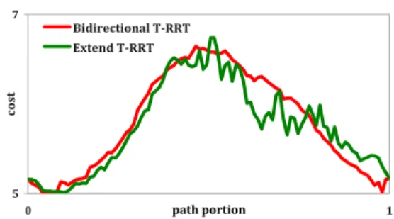
Cost Profiles: The cost profiles of paths obtained on the Manipulator problem reveal why the Bidirectional T-RRT can improve path quality (cf. Fig. 6). When T-RRT starts a descending phase after passing a saddle point, temperature is high because of the previous ascension, making the transition test less selective: uphill moves are accepted on the way down. The produced path is then a succession of downhill and uphill steps, leading to a jerky cost profile. On the contrary, when T-RRT is on an ascending phase, it is hard to go on: few uphill moves are accepted from a given node. But, these moves enable to reach the saddle point and appear in the extracted path. An ascending path is thus a rather smooth succession of uphill moves, as can be seen in Fig. 6 for the first half of both cost profiles. Furthermore, with the Bidirectional T-RRT, the second half is also an ascending one, but performed by the second tree. Taken in reverse direction, it appears as a smooth descent.
Tree Growth Bias: Besides its tree-linking role, the junction procedure proposed in [1] introduces a bias in the search process: at each iteration, one tree is potentially grown
5 7 0 path portion 1 co st Bidirectional T‐RRT Extend T‐RRT
Fig. 6. Cost profiles of two paths produced on the Manipulator problem by the Extend and Bidirectional T-RRT respectively. These paths are representative in the sense that their associated cost measurements are close to average values obtained over 100 runs. Cost profiles obtained with the Goal-biasedand Connect T-RRT are similar to that of the Extend T-RRT.
toward a new node from the other tree. While using the tree-linking mechanism presented in Algorithm 5, we evaluated the impact of this bias. For that, at each iteration, if a new node was created in the tree Ta, and if the junction to Tb
failed, we attempted to grow Tb toward the new node in Ta
using the Extend function. After evaluation, this bias appears to increase running time on some problems and to globally decrease path quality.
Common Expansion Direction: We also evaluated a variant of the Bidirectional T-RRT in which, at each iteration, both trees are grown toward the same random configuration, and up to two junctions are attempted depending on the number of new nodes. This variant appears to be less efficient than the one presented in Algorithm 4. Its running time is slightly higher because of the greater number of attempted junctions. More importantly, the quality of the paths produced is globally reduced.
Balanced Trees and Local Temperature: Finally, we evaluated two other versions of the Bidirectional T-RRT. The first one, which has proven to be beneficial to RRT on some problems, consists of ensuring that both trees remain balanced (in terms of number of nodes). The second one is specific to T-RRT and involves having a separate temperature associated to each tree. After evaluation, it is unclear whether these modifications are advantageous or not. They both appear to have sometimes a positive impact and sometimes a negative impact on performance.
Comparison with RRT*: We implemented RRT* so that it minimized the mechanical work of a path, which has been shown to be a good criterion to assess path quality [8]. As it is the quality criterion T-RRT tends to minimize, a fair comparison with RRT* must be based on the mechanical work. Results of this comparison are shown in Fig. 7. On the Mountains problem, RRT* quickly finds a better solution than T-RRT, even though the Bidirectional T-RRT performs equally well for 0.1 s. On the Stones problem, RRT* cannot find a solution in less than 0.5 s, contrary to the Bidirectional T-RRT, which succeeds in 0.1 s; but, given enough time, RRT* converges toward a better solution. On the Manipulator and Inspection problems involving a 6-DoF manipulator arm, even in its Extend form, T-RRT outperforms RRT*. As pointed out in [11], RRT* converges very slowly, except on 2D problems.
Mountains 0 5 10 15 20 25 30 35 0 1 2 3 t (s) MW RRT* Extend T‐RRT Bidirectional T‐RRT Stones 0 25 50 75 100 125 150 175 0 2 4 6 t (s) RRT* Extend T‐RRT Bidirectional T‐RRT Manipulator 0 2 4 6 8 10 12 0 2 4 6 8 t (s) RRT* Extend T‐RRT Bidirectional T‐RRT Inspection 0 200 400 600 800 1000 1200 1400 0 50 100 150 200 t (s) RRT* Extend T‐RRT Bidirectional T‐RRT
Fig. 7. Path cost (measured by the mechanical work M W ) versus running time (t, in seconds) for solution paths produced by T-RRT and RRT*. For each segment representing T-RRT, the left point corresponds to Trate= 0.1 and the right point to Trate= 0.01. Values are averaged over 100 runs.
VI. INDUSTRIALINSPECTIONPROBLEM
This section presents a path planning problem for a flying robot in a dense industrial environment, as illustrated by Fig. 1. For safety reasons, the quadrotor has to move in this environment trying to maximize its distance to obstacles. This scenario is an example of an industrial inspection problem involving aerial robots, such as those addressed in the framework of the ARCAS project (http://www.arcas-project.eu). One of the goals of this project is to develop robot systems for the inspection and maintenance of indus-trial installations difficult to access for humans.
In this example, the quadrotor is modeled as a 3-DoF sphere (i.e. a free-flying sphere) representing the safety zone around it; therefore, no visibility constraint is considered. We assume that the motions of the quadrotor are performed quasi-statically, thus neglecting dynamic constraints. We restrict the problem to planning in position, controllability issues being out of the scope of this paper.
When running the Extend T-RRT on this problem, we observed that only 38 of the 100 runs succeeded in less than five minutes with Trate = 0.1, and 67 with Trate = 0.01.
The success rate was even lower for the Connect T-RRT. On the other hand, the Bidirectional T-RRT can find a solution in less than 3 s (on average over 100 runs) when Trate= 0.1,
and in about 38 s when Trate = 0.01. The Goal-biased
T-RRT is about twice faster, but produces lower-quality paths, with cost measurements up to 30% higher. The example trajectory in Fig. 1 is typical of what the Bidirectional T-RRT produces when Trate = 0.01: it shows that the quadrotor
follows a convoluted path in order to maximize clearance. When Trate = 0.1, solution paths are more diverse, some
being shorter but having a lower clearance. VII. CONCLUSION
We have presented several enhancements to the T-RRT algorithm. First, we have described how its transition test can be modified to improve performance. Then, we have an-alyzed various extensions inspired by classical RRT variants. We have shown that the Goal-biased and Connect T-RRT are delicate to use because, despite reducing running time, they sometimes decrease path quality. Moreover, naively applying the Bidirectional paradigm as defined for RRT yields poor-quality solution paths. Thus, we have developed a specific Bidirectional variant to T-RRT, and we have shown that it improves performance compared to the Extend T-RRT,
mainly in terms of success rate and running time, but also often in terms of path quality. It does not always outperform the Goal-biased and Connect T-RRT, but it provides more consistent results and is therefore a better choice. Finally, we have illustrated the need to enhance T-RRT with a realistic industrial inspection problem. In such a context, the Extend T-RRT cannot find a solution in a reasonable amount of time, contrary to the Bidirectional T-RRT.
In the short future, we aim to investigate further im-provements and extensions of T-RRT. In particular, more sophisticated heuristics for the adaptive variation of the temperature parameter could lead to a faster exploration while maintaining path quality. We are also investigating a multiple-tree approach, similar to proposed extensions of RRT (see e.g. [16]), to enable the effective application of T-RRT to highly-complex problems in very large workspaces.
REFERENCES
[1] S. M. LaValle and J. J. Kuffner, “Rapidly-exploring random trees: Progress and prospects,” in Algorithmic and Computational Robotics: New Directions. A K Peters, 2001.
[2] C. Urmson and R. Simmons, “Approaches for heuristically biasing RRT growth,” in Proc. IROS, 2003.
[3] D. Ferguson and A. Stentz, “Anytime RRTs,” in Proc. IROS, 2006. [4] ——, “Anytime, dynamic planning in high-dimensional search
spaces,” in Proc. IEEE ICRA, 2007.
[5] A. Ettlin and H. Bleuler, “Rough-terrain robot motion planning based on obstacleness,” in Proc. ICARCV, 2006.
[6] ——, “Randomised rough-terrain robot motion planning,” in Proc. IROS, 2006.
[7] J. Lee, C. Pippin, and T. R. Balch, “Cost based planning with RRT in outdoor environments,” in Proc. IROS, 2008.
[8] L. Jaillet, J. Cort´es, and T. Sim´eon, “Sampling-based path planning on configuration-space costmaps,” IEEE Trans. Robot., vol. 26 (4), 2010. [9] J. Mainprice, E. A. Sisbot, L. Jaillet, J. Cort´es, R. Alami, and T. Sim´eon, “Planning human-aware motions using a sampling-based costmap planner,” in Proc. IEEE ICRA, 2011.
[10] D. Berenson, T. Sim´eon, and S. S. Srinivasa, “Addressing cost-space chasms in manipulation planning,” in Proc. IEEE ICRA, 2011. [11] R. Iehl, J. Cort´es, and T. Sim´eon, “Costmap planning in high
dimen-sional configuration spaces,” in Proc. IEEE/ASME AIM, 2012. [12] L. Jaillet, F. J. Corcho, J.-J. P´erez, and J. Cort´es, “Randomized tree
construction algorithm to explore energy landscapes,” J. Comput. Chem., vol. 32 (16), 2011.
[13] S. Karaman and E. Frazzoli, “Sampling-based algorithms for optimal motion planning,” Int. J. Robot. Res., vol. 30 (7), 2011.
[14] J. C. Spall, Introduction to Stochastic Search and Optimization: Estimation, Simulation, and Control. Wiley, 2003.
[15] T. Sim´eon, J.-P. Laumond, and F. Lamiraux, “Move3D: A generic platform for path planning,” in Proc. IEEE ISATP, 2001.
[16] E. Plaku, K. E. Bekris, B. Y. Chen, A. M. Ladd, and L. E. Kavraki, “Sampling-based roadmap of trees for parallel motion planning,” IEEE Trans. Robot., vol. 21 (4), 2005.