Alzheimer’s Disease Detection in Brain Magnetic Resonance Images Using Multiscale Fractal Analysis

(1)

Volume 2013, Article ID 627303,7pages http://dx.doi.org/10.5402/2013/627303

Research Article

Alzheimer’s Disease Detection in Brain Magnetic Resonance

Images Using Multiscale Fractal Analysis

Salim Lahmiri and Mounir Boukadoum

Department of Computer Science, University of Quebec at Montreal, 201 President-Kennedy, Local PK-4150, Montreal, QC, Canada H2X 3Y7

Correspondence should be addressed to Mounir Boukadoum; boukadoum.mounir@uqam.ca Received 15 July 2013; Accepted 19 September 2013

Academic Editors: P. A. Narayana and K. Tsuchiya

Copyright © 2013 S. Lahmiri and M. Boukadoum. This is an open access article distributed under the Creative Commons Attribution License, which permits unrestricted use, distribution, and reproduction in any medium, provided the original work is properly cited.

We present a new automated system for the detection of brain magnetic resonance images (MRI) affected by Alzheimer’s disease (AD). The MRI is analyzed by means of multiscale analysis (MSA) to obtain its fractals at six different scales. The extracted fractals are used as features to differentiate healthy brain MRI from those of AD by a support vector machine (SVM) classifier. The result of classifying 93 brain MRIs consisting of 51 images of healthy brains and 42 of brains affected by AD, using leave-one-out cross-validation method, yielded99.18% ± 0.01 classification accuracy, 100% sensitivity, and 98.20% ± 0.02 specificity. These results and a processing time of 5.64 seconds indicate that the proposed approach may be an efficient diagnostic aid for radiologists in the screening for AD.

1. Introduction

Alzheimer’s disease (AD) is a progressive and degenera-tive disease that affects brain cells, and its early diagnosis has been essential for appropriate intervention by health professionals. Noninvasive in vivo neuroimaging techniques such as magnetic resonance imaging (MRI) and positron emission tomography (PET) are commonly used to diagnose and monitor the progression of the disease and the effect of treatment. In this regard, the problem of developing computer aided diagnosis (CAD) tools to distinguish images with AD from those of normal brains has been extensively

addressed in the past years [1–12]. A review of a recent work

follows.

Magnin et al. [1] used the relative weight of gray matter

versus white matter and cerebrospinal fluid in 90 regions of interests (ROI) as features classified with SVM. Based on the bootstrap method, the SVM obtained 94.5% average classification accuracy in the classification of 16 AD and 22 control (healthy) subjects, with a mean specificity of 96.6%

and a mean sensitivity of 91.5%. Ram´ırez et al. [2] proposed a

classification system for AD based on the partial least square (PLS) regression model for feature extraction (identification

of discriminative voxels) and the random forest (RF) clas-sifier. The PLS-RF system yielded accuracy, sensitivity, and specificity values of 96.9%, 100%, and 92.7%, respectively, after classifying 41 normal and 56 AD images using the

leave-one-out cross-validation method. Salas-Gonzalez et al. [3]

used Welch’s 𝑡-test to identify voxels that provide higher

difference between normal and AD images. The identified voxels formed the main features to classify, and a SVM with linear kernel reached 96.2% accuracy in distinguishing 41 normal and 38 AD images using leave-one-out cross-validation method; the sensitivity and the specificity were

about 96%. Chincarini et al. [4] sampled the brain with seven

relatively small volumes that were filtered to give intensity and textural MRI-based features. Each filtered region was analyzed with a random forest classifier to extract relevant features, which were subsequently processed with a support vector machine. The system performance was evaluated on the classification of 144 AD patients and 189 controls. Using receiver operating curve (ROC) analysis for 144 AD patients and 189 controls, and 20-fold cross-validation, the result was 0.97 area under curve (AUC) for discriminating the AD images from the normal ones, with 89% sensitivity and 94%

(2)

analysis to classify subjects with Alzheimer’s disease and normal subjects. The Pearson product moment correlation coefficients were used to assess the connectivity between ROI in the brain. Classification of the AD group (20 subjects) and the non-AD group (20 subjects) using leave-one-out cross-validation led to 87% AUC, 85% sensitivity, and 80%

speci-ficity. Gra˜na et al. [6] used fractional anisotropy of diffusion

tensor imaging (DTI) data to obtain information about the magnitude of the water diffusion process at each voxel. Based on leave-one-out cross-validation method, the linear kernel SVM achieved overall accuracy of 100% for the classification of 25 healthy controls and 20 AD images. Wolz et al.

[7] used the hippocampal volume (HV), cortical thickness

(CTH), tensor-based morphometry (TBM), and features extracted from manifold-based learning (MBL) framework to discriminate healthy controls (231 subjects) from subjects with AD (198 subjects). Five percent of the evaluation subjects were kept for testing and the remaining 95% were used for training. The SVM achieved 86% correct classification

rate, 94% sensitivity, and 78% specificity. Zhang et al. [8]

proposed a multimodal data fusion and classification method based on features extracted from structural MRI, functional imaging (FDG-PET), and cerebrospinal fluid (CSF). The three modalities were, respectively, used to measure brain atrophy and to quantify hypometabolism and specific pro-teins linked to AD. Consequently, 93 volumetric features were extracted from 93 ROI automatically labeled by an atlas warping algorithm. The linear SVM was used to evaluate the classification accuracy using 10-fold cross-validation. The result of classifying 51 AD and 52 normal controls yielded classification accuracy of 93.2%, with a sensitivity of 93%

and a specificity of 93.3%. Daliri [9] used the scale-invariant

feature transforms (SIFT) to extract features from MR images

that were clustered using the 𝐾-means algorithm. Fisher’s

discriminant ratio was used for ranking clustered features, and genetic algorithms performed feature subset selection. The validation data consisted of the MRIs from 98 normal subjects and from 100 subjects with AD. The SVM achieved 86% correct classification rate using leave-one-out

cross-validation method. Gray et al. [10] combined cross-sectional

and longitudinal FDG-PET information for classification. Particularly, the whole brain was segmented into 83 anatom-ically defined regions from which intensities and changes in signal intensity over the follow-up period were extracted. The SVM achieved a classification accuracy of 88% for 200 patients with Alzheimer’s disease and 200 healthy controls

using fivefold cross-validation protocol. Li et al. [11] used

longitudinal changes of cortical thickness to characterize AD pathology. In particular, three categories of features were extracted from each subject, including static cortical thick-ness, cortex thinning dynamics, and the correlation between the longitudinal thickness changes of different regions of interest (ROI) in brain image. Based on leave-one-out cross-validation method, the SVM distinguished 37 AD patients from 40 NC with an accuracy of 96.1%.

In a recent work, we proposed a fractal-based processing

methodology to detect AD in brain MRI [12]. The system

does not require image reduction or segmentation, and it relies on a simple three-step algorithm. First, the brain MRI

is transformed into a one-dimensional (1D) signal by row concatenation. Then, a three-component feature vector is extracted from the 1D signal to characterize its local and global fractal features as expressed by Hurst’s exponent and the two results from the detrended fluctuation analysis (DFA)

[13] of the cumulated 1D signal: the scaling exponent and the

total detrended fluctuation energy (Hurst’s exponent allows the evaluation of how a signal is self-affine, i.e., can be made self-similar by an affine transformation for a given level of detail (a self-similar image is one whose whole is similar to its parts); DFA is a generalization that can also detect long-range power-law correlations in seemingly nonstationary

signals [13]. In particular, it can determine local trends in

the signal and measure its level of persistence). In the last step, the obtained feature vector is classified by a SVM with polynomial kernel. The validation with 10 normal brain MRI and 13 corresponding to AD led to 100% classification accuracy by a SVM with quadratic kernel. The obtained results suggested that the use of fractals to characterize the MRI of normal patients and ones with AD held the promise of equal or better classification accuracy than the best alternative approach while being simpler to implement.

The perfect classification accuracy reported in [12] was

encouraging. However, it was achieved with a small set of MRI for validation. In addition, the average processing time to extract the fractal features took over 400 seconds. This

paper follows up the work in [12] with a faster algorithm

and a bigger database for validation. First, the features extraction processing time is reduced considerably by using

multiscale analysis (MSA) [14] as alternative for Hurst’s and

DFA exponent estimation. Indeed, the approach reported

by Lahmiri and Boukadoum in [12] determines the sought

exponents by running polynomial regressions on multiple boxes or intervals of the 1D signal; on the other hand, MSA

uses the generalized Hurst’s exponent method [14], which

determines the scaling properties of the signal by computing

the 𝑞th-order moments of the distribution of the signal’s

increments [14]. This method combines the sensitivity to

any type of signal dependence with a high computational

efficiency due to its simple algorithm [14]. As each scale

𝑞 allows the estimation of a Hurst’s exponent, varying this value allows obtaining the multifractals of the signal in a straightforward way.

An additional contribution of this work is the use of a relatively larger database for validation in comparison to

[12]. Finally, our approach does not require a predetermined

region of interest as done in [1,5,8,10] and avoids extracting a

large number of features to characterize the image in different

modalities as done in [3,4,6–9,11]. Instead, the multifractal

analysis is performed on the whole brain MR image, and the extracted fractals are used to distinguish AD images from normal ones by the support vector machine. The SVM is a pattern recognition technique based on the statistical learning theory that finds the optimal nonlinear hyperplane

that minimizes the expected classification error [15]. It was

successfully applied in previous works [1,3,6,8–12].

The balance of this paper is as follows.Section 2presents

the multiscale analysis used to obtain the generalized Hurst’s exponents used to characterize brain MR images and

(3)

the SVM used for classification. InSection 3, we describe the obtained classification performance in terms of the accuracy rate, sensibility, and sensitivity. Finally, our conclusions are

drawn inSection 4.

2. Material and Methods

2.1. Image Database. A collection of 93 axial, T2-weighted

MR brain images of256 × 256 size were downloaded from

the Harvard Medical School webpage [16]. The set included

51 images of normal (healthy) brains and 42 of abnormal (unhealthy) brains affected by AD. We notice that there is no indication in the database regarding the AD stage.

Figure 1shows examples of healthy and AD images used in the experiments.

2.2. Multiscaling Analysis. Consider a signal𝑆(𝑡) defined at

discrete time intervals𝑡 = V, 2V, . . . , 𝑇 over a period 𝑇 that

is an integer multiple ofV. The 𝑞th-order moments of the

distribution that characterize the statistical evolution of𝑆(𝑡)

are defined as follows [17]:

𝐾_𝑞(𝑑) =⟨‖𝑆 (𝑡 + 𝑑) − 𝑆 (𝑡)‖𝑞⟩

⟨|𝑆 (𝑡)|𝑞_⟩ , (1)

where𝑑 ∈ [V, 𝑑_max] is a time interval and 𝑑_maxis its

predeter-mined upper limit. The generalized Hurst’s exponent𝐻(𝑞) is

defined from the scaling behavior of𝐾_𝑞(𝑑) according to the

following empirical relation [17]:

𝐾_𝑞(𝑑) ∝ (𝑑

V)

𝑞𝐻(𝑞)

. (2)

If𝐾_𝑞(𝑑) and 𝑑 satisfy a linear relationship for a given order

𝑞 in log-log scale, Hurst’s exponent 𝐻(𝑞) can be estimated

by running a linear regression of log(𝐾_𝑞(𝑑)) versus log(𝑑).

The generalized Hurst’s exponent𝐻(𝑞) describes the

long-memory dependence or persistence in the signal𝑆(𝑡). The

multiscaling structure of signal 𝑆(𝑡) is related to different

orders𝑞 of the exponent 𝐻(𝑞). In general, when 𝐻(𝑞) > 0.5,

the signal fluctuations related to the order𝑞 are persistent.

When𝐻(𝑞) < 0.5, the signal fluctuations related to order

𝑞 are antipersistent. Finally, the signal fluctuations are those

of a random walk if𝐻(𝑞) = 0.5 [17]. Notice that𝐻(𝑞 = 2)

corresponds to the classic Hurst’s exponent [14].

In this paper, the range of 𝑞 is arbitrarily fixed to the

interval from 1 to 6. Higher moments could also have been

considered as will be discussed inSection 4.

The original MRI is transformed into a one-dimensional (1D) signal by row concatenation. Then, Hurst’s exponents 𝐻(𝑞) for 𝑞 = 1, . . . , 6 are estimated by applying the MSA algorithm. The resulting six-component feature vector forms the input of the SVM classifier to perform the identification of AD images.

2.3. The Support Vector Machine Classifier. Introduced by

Vapnik [15], the support vector machine (SVM) classifier

is based on statistical learning theory. It implements the principle of structural risk minimization and has excellent

generalization ability as a result, even when the data sample is small. The SVM performs a classification tasks by con-structing an optimal separating hyperplane that maximizes the margin between the two nearest data points belonging

to two separate classes. Given a training set {(𝑥_𝑖, 𝑦_𝑖), 𝑖 =

1, 2, . . . , 𝑚}, where the input 𝑥_𝑖 ∈ 𝑅𝑑 _{and class labels}_𝑦

𝑖 ∈

{+1, −1}, the separation hyperplane for a linearly separable binary classification problem is given by

𝑓 (𝑥) = ⟨𝑤 ⋅ 𝑥⟩ + 𝑏, (3)

where 𝑤 is a weight vector and 𝑏 is a bias. The optimal

separation hyperplane is found by solving the following optimization problem: Minimize 𝑤,𝑏,𝜉 1 2⟨𝑤 ⋅ 𝑤⟩ + 𝐶 𝑚 ∑ 𝑖=1 𝜉_𝑖 (4) subject to 𝑦𝑖(⟨𝑤 ⋅ 𝑥𝑖⟩ + 𝑏) + 𝜉𝑖− 1 ≥ 0, 𝜉𝑖≥0, (5)

where 𝐶 is a penalty parameter that controls the tradeoff

between the complexity of the decision function and the

number of misclassified training examples and𝜉 is a positive

slack variable. The previous optimization model can be solved by introducing Lagrange multipliers and using the Karush-Kuhn-Tucker theorem of optimization to obtain the solution as

𝑤 =∑𝑚

𝑖=1

𝛼_𝑖𝑦_𝑖𝑥_𝑖. (6)

The𝑥_𝑖values corresponding to positive Lagrange multipliers

𝛼_𝑖 are called support vectors, and they define the decision

boundary. The𝑥_𝑖values corresponding to zero𝛼_𝑖are

irrele-vant. Once the optimal values of𝛼, 𝛼∗are found, the optimal

hyperplane parameters𝑤∗and𝑏∗are determined. Then, the

discriminant function of the SVM for a linearly separable binary classification problem is given by

𝑔 (𝑥) = sign (∑𝑚

𝑖=1

𝑦_𝑖𝛼∗_𝑖 ⟨𝑥_𝑖⋅ 𝑥⟩ + 𝑏∗) . (7)

In the nonlinearly separable case, the SVM classifier nonlin-early maps the training points to a high dimensional feature

space using a kernel functionΦ, where linear separation can

be possible. The scalar product⟨Φ(𝑥_𝑖) ⋅ Φ(𝑥_𝑗)⟩ is computed

by Mercer kernel function𝐾 as 𝐾(𝑥_𝑖, 𝑥_𝑗) = ⟨Φ(𝑥_𝑖) ⋅ Φ(𝑥_𝑗)⟩.

Then, the nonlinear SVM classifier has the following form:

𝑔 (𝑥) = sign (∑𝑚

𝑖=1

𝑦_𝑖𝛼_𝑖∗𝐾 ⟨𝑥, 𝑥_𝑖⟩ + 𝑏∗) . (8)

In this study, a polynomial kernel of degree 2 was used for the SVM. As a global kernel, it allows data points that are far away from each other to also have an influence on the kernel values. The general polynomial kernel is given by

(4)

(a) (b) Figure 1: Healthy image (a) and AD image (b) in grayscale.

Brain

MRI Concatenate rows 1D signal Apply MSA

Compute SVM Features vector

Classification

H(q)

Figure 2: AD diagnosis system.

where𝑑 is the order of the polynomial to be used. In this

study, it was varied from 2 to 4. Higher orders were ignored because of a higher computational burden with no substantial gain in classification accuracy from our experience.

2.4. Validation. The design of the automated AD diagnosis

system is shown inFigure 2.

The validation experiments were conducted using the leave-one-out cross-validation method. Then, the average and standard deviation of the correct classification rate (CCR), sensitivity, and specificity were computed to evaluate the performance of the classifier. The three performance measures are defined as follows:

CCR= Classified Samples

Total Number of Samples,

Sensitivity= Correctly Classified Positive Samples

True Positive Samples ,

Specificity= Correctly Classified Negative Samples

True Negative Samples ,

(10) where positive samples and negative samples refer to AD and normal images, respectively.

3. Results

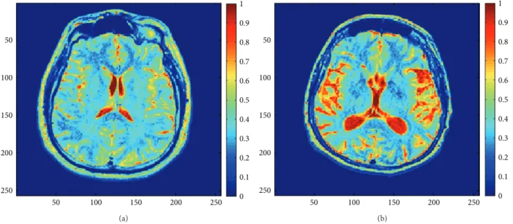
Before processing, the grayscale images as shown inFigure 1

are converted to double color format to perform MSA (see

examples inFigure 3).Figure 4shows the obtained behavior

of𝐾_𝑞(𝑑) as a function of 𝑑 (see, (2)) for the images of healthy

patients and those with AD and for𝑞 varying from 1 to 6,

whereas 𝑑 varies from 1 to 19. Figure 5provides the same

information on a log-log scale.Figure 4reveals that, for the

images of normal brains,𝐾_𝑞(𝑑) quickly reaches horizontal

saturation for𝑞 = 1, 2, 3; this is not so for the AD images

where𝐾_𝑞(𝑑) increases monotonically for all 𝑑. In addition,

the magnitude of𝐾_𝑞(𝑑) for a healthy image is in general larger

than that of an AD image. In summary, Hurst’s exponents appear to be different at each scale for the two types of brain MRIs.

As mentioned previously, the order of the polynomial kernel used in the SVM was varied from 2 to 4. The best classification performance was obtained with a fourth-order kernel, for which the correct classification rate, sensitivity,

and specificity were99.18% ± 0.0083, 100%, and 98.20% ±

0.0182, respectively. A visual analysis of the AD images revealed that seventeen of them looked markedly different

from the example inFigure 1(Figure 6shows three of them).

Removing them from the validation database led to 100% classification accuracy by the SVM.

(5)

50 100 150 200 250 50 100 150 200 250 0 0.1 0.2 0.3 0.4 0.5 0.6 0.7 0.8 0.9 1 (a) 50 100 150 200 250 50 100 150 200 250 0 0.1 0.2 0.3 0.4 0.5 0.6 0.7 0.8 0.9 1 (b) Figure 3: Healthy image (a) and AD image (b) in double color format.

0 2 4 6 8 10 12 14 16 18 0 0.2 0.4 0.6 0.8 1 1.2 1.4 1.6 1.8 2 d Kq (d ) q = 1 q = 2 q = 3 q = 4 q = 5 q = 6 (a) 0 0.2 0.4 0.6 0.8 1 1.2 1.4 Kq (d ) 0 2 4 6 8 10 12 14 16 18 d q = 1 q = 2 q = 3 q = 4 q = 5 q = 6 (b)

Figure 4: Multiscale analysis results of healthy image (a) and AD (b).

Finally, the MSA running time was 5.64 seconds, and the overall image processing time was about 8 seconds on a 3.30 GHz Core i5-2500 CPU using MATLAB 2012a codes, leading to an execution speed improvement of nearly two orders of magnitude in comparison to Hurst’s exponent and DFA.

4. Discussion and Conclusion

The overall classification accuracy obtained in this work was 99.18% ± 0.01. However, excluding some atypical AD images led to 100% correct classification rate. This suggests that a multi-SVM approach, where one or more classifier handles

the misclassified images by the first SVM, might lead to perfect classification accuracy in all situations. We intend to investigate this possibility.

Our approach for AD detection outperformed most of the studies found in the literature, where the reported

clas-sification accuracy was between 86% and 96.9% [1–5,7–13].

One exception is the work of [6] where perfect classification

accuracy is reported. However, it is achieved with a database on only 45 MR images (25 healthy controls and 20 AD images), and the number of features used was higher than 1000 in comparison to the six used by our approach. We limited the number of features to six somewhat arbitrarily, and we have not investigated the effect of more or less features

(6)

log(d) log (K q (d )) 10−2 10−1 100 101 100 101 q = 1 q = 2 q = 3 q = 4 q = 5 q = 6 (a) log(d) log (K q (d )) 10−2 10−1 100 101 10−3 100 101 q = 1 q = 2 q = 3 q = 4 q = 5 q = 6 (b)

Figure 5: Multiscale analysis results on log-log scale of healthy image (a) and AD (b).

Figure 6: Examples of excluded AD images in the second experiment.

on the performance of the classifier. Future work should also investigate this.

In summary, multiscale analysis-based Hurst’s exponents were used for the classification of healthy brain images versus AD by a SVM with fourth-order kernel. The obtained results show the potential of using multiscale fractal analysis to differentiate healthy brain images from ones affected by Alzheimer’s disease. The MSA algorithm took 5.64 seconds to analyze a brain MRI while the detrended fluctuation

analysis (DFA) took 400 seconds in our previous work [12].

In addition, a larger database is used for validation.

Finally, although we have obtained better result than the literature in general, it is difficult to draw definite conclusions since we used a different image database. In future work, we will explore a benchmark image depository such as the Alzheimer’s Disease Neuroimaging Initiative (ADNI) database. Furthermore, we will investigate the effectiveness of MSA to classify AD images versus mild cognitive impairment (MCI). Indeed, the ability to correctly classify the AD and MCI images based on MSA Hurst’s exponents might shed

light on the ability to predict the conversion from MCI to AD, which is of clinical interest.

References

[1] B. Magnin, L. Mesrob, S. Kinkingn´ehun et al., “Support vec-tor machine-based classification of Alzheimer’s disease from whole-brain anatomical MRI,” Neuroradiology, vol. 51, no. 2, pp. 73–83, 2009.

[2] J. Ram´ırez, J. M. G´orriz, F. Segovia et al., “Computer aided diagnosis system for the Alzheimer’s disease based on partial least squares and random forest SPECT image classification,”

Neuroscience Letters, vol. 472, no. 2, pp. 99–103, 2010.

[3] D. Salas-Gonzalez, J. M. G´orriz, J. Ram´ırez et al., “Computer-aided diagnosis of Alzheimer’s disease using support vector machines and classification trees,” Physics in Medicine and

Biology, vol. 55, no. 10, pp. 2807–2817, 2010.

[4] A. Chincarini, P. Bosco, P. Calvini et al., “Local MRI analysis approach in the diagnosis of early and prodromal Alzheimer’s disease,” NeuroImage, vol. 58, no. 2, pp. 469–480, 2011.

(7)

[5] G. Chen, B. D. Ward, C. Xie et al., “Classification of Alzheimer disease, mild cognitive impairment, and normal cognitive status with large-scale network analysis based on resting-state functional MR imaging,” Radiology, vol. 259, no. 1, pp. 213–221, 2011.

[6] M. Gra˜na, M. Termenon, A. Savio et al., “Computer aided diag-nosis system for Alzheimer disease using brain diffusion tensor imaging features selected by Pearson’s correlation,” Neuroscience

Letters, vol. 502, no. 3, pp. 225–229, 2011.

[7] R. Wolz, V. Julkunen, J. Koikkalainen et al., “Multi-method analysis of MRI images in early diagnostics of Alzheimer’s disease,” Plos One, vol. 6, no. 10, Article ID e25446, 2011. [8] D. Zhang, Y. Wang, L. Zhou, H. Yuan, and D. Shen, “Multimodal

classification of Alzheimer’s disease and mild cognitive impair-ment,” NeuroImage, vol. 55, no. 3, pp. 856–867, 2011.

[9] M. R. Daliri, “Automated diagnosis of Alzheimer disease using the scale-invariant feature transforms in magnetic resonance images,” Journal of Medical Systems, vol. 36, no. 2, pp. 995–1000, 2012.

[10] K. R. Gray, R. Wolz, R. A. Heckemann, P. Aljabar, A. Hammers, and D. Rueckert, “Multi-region analysis of longitudinal FDG-PET for the classification of Alzheimer’s disease,” NeuroImage, vol. 60, no. 1, pp. 221–229, 2012.

[11] Y. Li, Y. Wang, G. Wu et al., “Discriminant analysis of longi-tudinal cortical thickness changes in Alzheimer’s disease using dynamic and network features,” Neurobiology of Aging, vol. 33, no. 2, pp. 427.e15–427.e30, 2012.

[12] S. Lahmiri and M. Boukadoum, “Automatic detection of Alzheimer disease in brain magnetic resonance images using fractal features,” in Proceedings of the 6th International IEEE

EMBS Conference on Neural Engineering, 2013.

[13] H. E. Stanley, L. A. N. Amaral, A. L. Goldberger, S. Havlin, P. C. Ivanov, and C.-K. Peng, “Statistical physics and physiology: monofractal and multifractal approaches,” Physica A, vol. 270, no. 1, pp. 309–324, 1999.

[14] T. Di Matteo, “Multi-scaling in finance,” Quantitative Finance, vol. 7, no. 1, pp. 21–36, 2007.

[15] V. Vapnik, The Nature of Statistical Learning Theory, Springer, Berlin, Germany, 1995.

[16] http://www.med.harvard.edu/AANLIB/.

[17] C. K. Peng, S. V. Buldyrev, S. Havlin, M. Simons, H. E. Stanley, and A. L. Goldberger, “Mosaic organization of DNA nucleotides,” Physical Review E, vol. 49, no. 2, pp. 1685–1689, 1994.

(8)

Submit your manuscripts at

http://www.hindawi.com

Stem Cells

International

Hindawi Publishing Corporation

http://www.hindawi.com Volume 2014

INFLAMMATION

Behavioural

Neurology

Endocrinology

International Journal of Hindawi Publishing Corporation

Disease Markers

BioMed

Research International

Oncology

Journal of

http://www.hindawi.com Volume 2014 Oxidative Medicine and Cellular Longevity Hindawi Publishing Corporation

PPAR Research

The Scientific

World Journal

Immunology Research

Journal of

Obesity

Journal of

http://www.hindawi.com Volume 2014 Computational and Mathematical Methods in Medicine

Ophthalmology

Journal of

Diabetes Research

Journal of

Research and Treatment

AIDS

Gastroenterology Research and Practice

Parkinson’s

Disease

Evidence-Based Complementary and Alternative Medicine Volume 2014 Hindawi Publishing Corporation