Open Archive TOULOUSE Archive Ouverte (OATAO)
OATAO is an open access repository that collects the work of Toulouse researchers and
makes it freely available over the web where possible.
This is an author-deposited version published in :
http://oatao.univ-toulouse.fr/
Eprints ID : 12343
To link to this article : DOI :10.4230/LIPIcs.TYPES.2011.55
URL :
http://dx.doi.org/10.4230/LIPIcs.TYPES.2011.55
To cite this version : Matthes, Ralph and Picard, Celia
Verification of
redecoration for infinite triangular matrices using coinduction
. (2013)
In: International Workshop on Types and Proofs for Programs -
TYPES 2011, 8 September 2011 - 11 September 2011 (Bergen,
Norway).
Any correspondance concerning this service should be sent to the repository
administrator:
[email protected]
Verification of redecoration for infinite triangular
matrices using coinduction
Ralph Matthes
1and Celia Picard
21 Institut de Recherche en Informatique de Toulouse (IRIT), C.N.R.S. and University of Toulouse, France
2 Institut de Recherche en Informatique de Toulouse (IRIT), University of Toulouse, France
Abstract
Finite triangular matrices with a dedicated type for the diagonal elements can be profitably represented by a nested data type, i. e., a heterogeneous family of inductive data types, while infinite triangular matrices form an example of a nested coinductive type, which is a heterogeneous family of coinductive data types.
Redecoration for infinite triangular matrices is taken up from previous work involving the first author, and it is shown that redecoration forms a comonad with respect to bisimilarity.
The main result, however, is a validation of the original algorithm against a model based on infinite streams of infinite streams. The two formulations are even provably equivalent, and the second is identified as a special instance of the generic cobind operation resulting from the well-known comultiplication operation on streams that creates the stream of successive tails of a given stream. Thus, perhaps surprisingly, the verification of redecoration is easier for infinite triangular matrices than for their finite counterpart.
All the results have been obtained and are fully formalized in the current version of the Coq theorem proving environment where these coinductive datatypes are fully supported since the version 8.1, released in 2007. Nonetheless, instead of displaying the Coq development, we have chosen to write the paper in standard mathematical and type-theoretic language. Thus, it should be accessible without any specific knowledge about Coq.
Keywords and phrases nested datatype, coinduction, theorem proving, Coq
1
Introduction
Redecoration for the finite triangles has been verified against a list-based model in previous work [10]. This is the point of departure for our present paper.
Finite triangles can be represented by “triangular matrices”, i. e., finite square matrices, where the part below the diagonal has been cut off. Equivalently, one may see them as sym-metric matrices where the redundant information below the diagonal has been omitted. The elements on the diagonal play a different role than the other elements in many mathematical applications, e. g., one might require that the diagonal elements are invertible (non-zero). This is modeled as follows: a type E of elements outside the diagonal is fixed throughout (we won’t mention it as parameter of any of our definitions), and there is a type of diagonal elements that enters all definitions as an explicit parameter. More technically, if A is the type of diagonal elements, then TrifinAshall denote the type of finite triangular matrices
with A’s on the diagonal and E’s outside (see Figure 1). Then, Trifin becomes a family of
© R. Matthes and C. Picard;
types, indexed over all types, hence a type transformation. Moreover, the different TrifinA
are inductive datatypes that are all defined simultaneously, hence they are an “inductive family of types” or “nested datatype” [4].
E E E E E E A A A A . . .
Figure 1 Dividing a triangle into columns
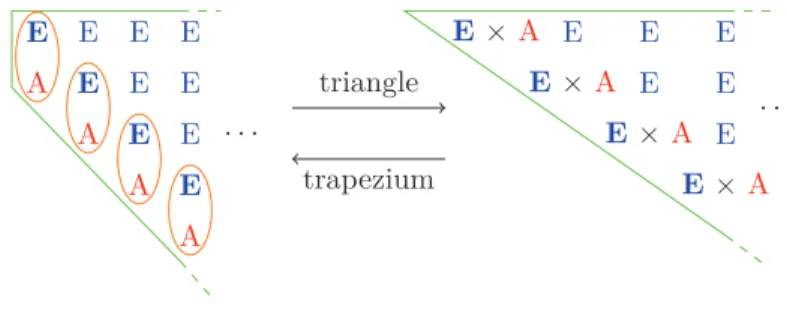
If we cut the triangle into the first column and the rest, we get one element of A and a “trapezium”, with an uppermost row solely consisting of E’s. In order not to have to ensure explicitly by a dependent type that the number of columns is coherent, the solution is to transform the trapezium into a triangle, integrating the side diagonal (just above the diagonal) into the diagonal itself, as shown in Figure 2. From the left to the right, the lowermost element of E in each column is paired with the element of A on the diagonal, and the other elements of E remain untouched.
E E E E E E A A A A E E E E . . . E E E E E E E×A E ×A E×A E×A . . . triangle trapezium Figure 2
Following this remark, the triangles can be defined theoretically [1], and in Coq and Isabelle by the following constructors [10]:
a: A
sgfina: TrifinA
a: A t: Trifin(E × A)
constrfina t: TrifinA
◮Remark. In this paper, single-lined inference rules denote inductive definitions, double-lined
inference rules are for coinductive definitions.
In more theoretical terms, Trifin is modeled as the least solution to the fixed-point
equation
TrifinA= A + A × Trifin(E × A)
The left summand corresponds to a triangle that only consists of a single element of A (a singleton), thus ensuring the base case.
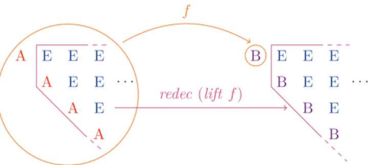
The algorithm of redecoration (see work by Uustalu and Vene for the general categorical notion [14]) is the following: for a given redecoration rule f : TrifinA→ B, it is a function
redec f that redecorates A-triangles t (elements of TrifinA) into B-triangles by applying f
to the whole triangle t to obtain the new top element, and then by successively applying the same operation to the triangle cut out from the remaining trapezium. This ends in the singleton case where f is applied to it and the result is turned into a triangle by applying
sgfin. This algorithm only changes the diagonal elements in A into elements of B, as shown
E E E E E E A A A A . . . E E E E E E B B B B . . . f Figure 3 Redecoration
The redecoration for infinite triangles [1] has not yet been verified. This is what we intend to do in this paper.
Reasoning about nested coinductive types naturally rests on observational equality, just as for ordinary coinductive types, and since version 8.2, Coq greatly helps in using the rewrite mechanism for Leibniz equality also for the notion of bisimilarity of infinite triangular matrices. With respect to that notion of equality, redecoration is shown to form a (sligthly weakened form of) comonad, and its implementation is compared with an alternative one based on streams of streams.
These new results come with a full formalization in Coq [9], and limitations of what Coq recognizes as a guarded definition make the theoretical development more challenging, but we still obtained smooth results without an excessive overhead that would be imposed by a naive dualization of the formalization for the finite triangles [10].
In Section 2, inspired by the previous theoretical development [1], we introduce the dual to the definition of finite triangles [10]. We present it with all the tools necessary to define redecoration. We then propose a definition for the redecoration algorithm on these infinite triangles and add further tools and properties. In Section 3, we change the point of view in the observation of the triangles. We give an alternative definition for the infinite triangles, considering this new approach, and provide various tools. We also show that this new representation is equivalent to the previous one. Finally, we propose two ways of defining redecoration, trying always to simplify and generalize our definitions and show their adequation with previous definitions.
Since the results are fully formalized in the current version of Coq, hence ensuring complete and sound proofs, we took the liberty to write the paper in standard mathematical and type-theoretic language and also to omit most proofs. Therefore, it should be accessible without any specific knowledge about Coq. For the study of the development [9], the Coq’Art book [3] should mostly suffice, but the (type) class mechanism [12] and the revised setoid rewriting mechanism based on it have to be consulted elsewhere – by default in the Coq Reference Manual [13].
2
Reference Representation with a Coinductive Family
Dually to the representation of finite triangles discussed in the introduction, “triangular matrices” are now introduced as infinite square matrices, where the part below the diagonal has been cut off. Recall that a type E of elements outside the diagonal is fixed throughout. If A is the type of diagonal elements, then Tri A shall denote the type of infinite triangular matrices with A’s on the diagonal and E’s outside. The different Tri A are coinductive datatypes that are all defined simultaneously, as was the case for Trifin, hence they are a
2.1
Infinite triangles as nested coinductive type
Infinite triangles can also be visualized as in Figure 1, this time with the dots representing an infinite extension.
If we now cut the triangle into the first column and the rest, we get one element of A (as before for Trifin) and a trapezium, with an uppermost row consisting of infinitely many E’s.
The n-th column consists of an element of A on the diagonal and n elements of E above the diagonal, as in the case of Trifin. As before, we do not want to parameterize the type of
the columns by their index and instead integrate the side diagonal into the diagonal – and this has to be done corecursively [1]. This integration is possible since trapeziums are again in one-to-one correspondence to triangles, as shown in Figure 2, now interpreted infinitely. In this figure, the trapezium to the left is considered as the “trapezium view” of the triangle to the right. Vice versa, the triangle to the right is the “triangle view” of the trapezium to the left.
We now formalize triangles through the following constructor that has to be interpreted coinductively.
◮Definition 1(Tri, defined coinductively).
a: A t: Tri(E × A)
constr a t: Tri A with A a type variable.
This means that the types Tri A for all types A are simultaneously conceived as greatest solution to the fixed-point equation
T ri A= A × Tri(E × A),
and constr has two arguments instead of a pair of type A × Tri(E × A) just for technical convenience.
The second argument to constr corresponds to the triangle view of the trapezium in our visualization in Figure 1, but there is no passage between a trapezium and a triangle – this is only the motivation. In the formalization, there are only infinite triangles, but we set
Trap A:= Tri(E × A) to hint to the trapezium view of these triangles.
◮Definition 2(Projections).
top: ∀A. Tri A → A rest : ∀A. Tri A → Trap A
top(constr a r) := a rest(constr a r) := r
This definition by pattern matching implicitly uses the direction from right to left in the above fixed-point equation. Thus, the top element and the trapezium part of a triangle are calculated by unfolding the fixed point.
In order to obtain the triangle that arises by cutting off the top row of a trapezium, we have to go through all the columns.
◮Definition 3(cut : ∀A.Trap A → Tri A, defined corecursively). cut(constr ée, aê r) := constr a (cut r)
The definition does pattern matching on elements of Trap A and constructs an element of the coinductive type Tri A. The subterm cut r represents a corecursive call to cut, which is accepted also by the Coq system as admissible corecursion since it is placed directly as an argument to the constructor constr.
2.2
Redecoration for infinite triangles
We are heading for a corecursive definition of the generic redecoration operation redec on triangles. It has type
∀A∀B. (Tri A → B) → Tri A → Tri B,
which is the type of a coextension operation for Tri viewed as support of a comonad. Coextension – also called cobind – is the dual of the extension / bind operation of a monad, which is so successfully used in the functional programming language Haskell. The counit for the comonad we are about to construct is our top operation.
Redecoration for Tri follows the same pattern as for Trifin, but the successive applications
of the same operation will never reach a base case, as there is none in Tri.
Formally, this is done by a corecursive definition, where redec f t for t of type Tri A has to call itself with second argument of type Trap A, hence f is not even type-correct as a first argument in that corecursive call. Instead of f : Tri A → B, a “lifted” version of f is needed that has type Tri(E × A) → E × B.
◮Definition 4(lift : ∀A∀B. (Tri A → B) → Tri(E × A) → E × B). lift f r:= éfst(top r), f (cut r)ê , where fst is the first projection (from a pair to its first component). The definition is illustrated in Figure 4.
E E E E E E A A A . . . E×B id f Figure 4 Definition of lifting
The formal definition of redecoration is as follows:
◮Definition 5(redec : ∀A∀B. (Tri A → B) → Tri A → Tri B, defined corecursively). redec f t:= constr (f t)!redec (lift f) (rest t)" ,
see Figure 5. This definition is accepted since it is guarded: the corecursive call to redec is as second argument to constr, and it does not matter that the argument f becomes lift f there. A function argument that becomes more complicated in the recursive call is typical of recursion on nested datatypes, see, e. g., [1].
This completes the definition, but leaves open the question if this is really (in what sense) the cobind of a comonad and if it corresponds to operations that are easier to understand than corecursion on nested codatatypes. We note that recursion schemes for nested datatypes have been subject of a long line of research, starting from work by Bird and colleagues [4, 5].
2.3
Properties of redecoration
It is well-known that propositional equality = (called Leibniz equality in Coq since t1= t2
E E E E E E A A A A . . . E E E E E E B B B B . . . f redec (lift f )
Figure 5 Definition of redecoration
the correctness of elements that are calculated in coinductive types. Propositional equality cannot be established by coinductive reasoning because this is confined to coinductively defined conclusions, and propositional equality is not coinductive (in Coq, it is defined inductively). We write Rel C for the type of the binary relations on C, and we use these relations in infix notation. In Coq, their type is C → C → Prop, where Prop is the universe of propositions.
◮Definition 6(≃ : ∀A. Rel(Tri A), defined coinductively).
t1, t2: Tri A top t1= top t2 rest t1≃ rest t2 t1 ≃ t2
It is easy to show that ≃ is an equivalence relation for any argument type A. It is an equivalence relation but not a congruence: for every operation of interest we have to establish compatibility with bisimilarity. This is in particular easily done for the projection functions
top and rest and for the cut operation.
Using this notion of bisimilarity, we can show that redec is extensional in its function argument (modulo ≃), using full extensionality of lift:
◮Lemma 7. ∀A∀B∀(f f′: Tri A → B). (∀t, f t = f′t) ⇒ ∀t, lift f t = lift f′t ◮Lemma 8. ∀A∀B∀(f f′: Tri A → B). (∀t, f t = f′t) ⇒ ∀t, redec f t ≃ redec f′t
The main properties of redec we are interested in express that top and redec together constitute a comonad for “functor” Tri. The precise categorical definition in coextension form (with a cobind operation instead of the traditional comultiplication) is, e. g., given in [14]. Here, we give the constructive notion we use in this paper, and it is parameterized by an equivalence relation while classically, only mathematical equality = is employed.
◮Definition 9(Constructive comonad). A constructive comonad consists of a type
transforma-tion T , a functransforma-tion counit : ∀A. T A → A, a functransforma-tion cobind : ∀A∀B.(T A → B) → T A → T B and an equivalence relation ≅ : ∀A. Rel(T A) such that the following comonad laws hold:
∀A∀B∀fT A→B∀tT A. counit(cobind f t) = f t (1) ∀A∀tT A
. cobind counitAt ≅ t (2)
∀A∀B∀fT A→B
∀gT B→C
∀tT A
. cobind(g ◦ cobind f ) t ≅ cobind g (cobind f t) (3) Here, in order to save space, we gave the type information for the term variables as superscripts. The index A to counit is meant to say that the type parameter to counit is set to A – in all other cases, we leave type instantiation implicit.
◮Definition 10(Constructive weak comonad). A constructive weak comonad is defined as a
constructive comonad, but where the equation in (3) is restricted to functions g that are compatible with ≅ in the following sense: ∀t t′
, t ≅ t′
⇒ g t = g t′
.
◮Lemma 11. The type transformation Tri, the projection function top and redec form a constructive weak comonad with respect to ≃.
The first comonad law is satisfied in an especially strong form: top(redec f t) actually is
f tby definition. The other comonad laws go through with suitable generalizations of the lemmas – in order to ensure guardedess of the proofs. The current solution is unspectacular, but it was not obvious how to do it (much more complicated solutions were found on the way and are now obsolete). We only show the strengthening of the second comonad law, but it is the same style for the third one.
◮Lemma 12(strengthened form of second comonad law for redec).
∀A∀(f : Tri A → A). (∀(t : Tri A), f t = top t) ⇒ ∀(t : Tri A). redec f t ≃ t
The proof is by coinduction and uses Lemma 7. Obviously, this implies the second comonad law. For all the details, see our formalization in Coq [9]. We only get a weak comonad because proving pointwise equality of lift(g ◦ (redec f )) and (lift g) ◦ (redec(lift f )) requires compatibility of g with ≃, and this is a crucial step for proving the third comonad law.
When defining the cut operation, one might naturally want to get also the part that has been cut out (the elements of E). These elements are given by the following function:
◮Definition 13(es_cut : ∀A. Trap A → Str E, defined corecursively). es_cut (constr ée, aê r) := e :: (es_cut r)
◮Remark. In the standard library of Coq, the type of streams with elements in type C are
predefined, and we can represent this definition as follows:
c: C s: Str C
c:: s : Str C
The projection functions are called hd and tl. They are such that hd(c :: s) = c and
tl(c :: s) = s. We will also use the map function defined by map f (c :: s) = f c :: (map f s). Using es_cut, we can define the first row of E elements in a triangle as
frow: ∀A. Tri A → Str E frow t:= es_cut (rest t)
Once we have these definitions, we might want to be able to “glue” the two cut parts in order to recreate the original trapezium. This is done by the function addes
◮Definition 14(addes : ∀A. Str E → Tri A → Trap A, defined corecursively). addes(e :: es) (constr a r) := constr ée, aê (addes es r) And it is then easy to show that addes indeed performs the gluing:
∀A∀(r : Trap A). addes (es_cut r) (cut r) ≃ r
3
Another Conception of Triangles
In this section, we show another way to perceive and represent infinite triangles. And we propose two ways of defining redecoration on this new representation.
3.1
A new definition using streams
In the previous section, we always visualized the infinite triangles by their columns. Indeed, we said that a triangle was a first column with only one element of type A (the element of the diagonal) and a trapezium, itself actually a triangle, as suggested in Figure 1.
While elements of the finite triangles in TrifinA(see Section 1) are (globally) finite, also
all the columns of our infinite triangles in Tri A are finite. In the work that we started from for this article [10], redecoration on Trifin is verified against a model where triangles are
represented by finite lists of columns, where each column consists of the diagonal element in
A and a finite list of elements in E. A naive dualization of that approach would consist in taking as representation of infinite triangles streams of columns that would be formed as for the finite ones. This mixture of inductive and coinductive datatypes is notoriously difficult to handle. We have been confronted with this problem many times in the last few years, as can be seen in the second author’s thesis [11] which deals with this kind of problems particularly in Coq. But in other proof assistants, the same kind of issues has appeared; there is also an experimental solution in Agda [6, 7]. Still, the representation of infinite triangles mixing inductive and coinductive datatypes can be carried out, but we refrain from presenting this column-based approach here.
However, we can also visualize triangles the other way around. We now consider the triangle by its rows, as suggested in Figure 6. Then, on any row, we have one element of
E E E E E E A A A A . . .
Figure 6 Dividing a triangle into rows
type A and infinitely many elements of type E. And we also have infinitely many rows. Here, nothing is finite (only the single element of A at the head of each row, but this is not a problem), therefore, we do not have any embedded inductive type in our description – unlike in the columnwise decomposition mentioned above. This new visualization can be represented as a stream of pairs made of one element of type A and a stream of elements of type E.
◮Definition 15. Tri′A:= Str(A × Str E)
Actually, following the definition of Str, we can read this new definition of the triangles as consisting of three parts: the top element, the stream of elements of E of the first row and the triangle corresponding to the rest, as shown in Figure 7.
E E E E E E A A A A . . . top′ frow′ rest′
Figure 7 Conceptualizing a triangle as a triple
◮Definition 16(Projections). top′ : ∀A. Tri′ A→ A frow′ : ∀A. Tri′ A→ Str E rest′ : ∀A. Tri′ A→ Tri′ A top′
(éa, esê :: t) := a frow′
(éa, esê :: t) := es rest′
(éa, esê :: t) := t Notice that rest and rest′
are conceptually different – the former yields the trapeziums after cutting off the first column, the latter triangles after cutting off the first row.
To compare two elements of Tri′
, we need a notion of bisimilarity, which on Str is pre-defined in Coq as follows:
◮Definition 17(≡ : ∀C. Rel(Str C), defined coinductively).
s1, s2: Str C hd s1= hd s2 tl s1≡ tl s2
s1 ≡ s2
However, we cannot use it directly. Indeed, we would need to prove, for two triangles t1 and t2that their first rows are Leibniz-equal, i. e., frow
′
t1= frow′
t2. This is too strict, since the rows are defined partially coinductively (because of the stream of E’s). Therefore, we need to define a new relation on Tri′
that will compare the three elements of the triangles. The tops can be compared through Leibniz equality, the first rows can be compared using ≡ and the rests with the relation on Tri′
, corecursively.
◮Definition 18(∼= : ∀A. Rel(Tri′A), defined coinductively). t1, t2: Tri′ A top′ t1= top′ t2 frow′ t1≡ frow′ t2 rest′ t1∼= rest′ t2 t1 ∼= t2
It is immediate to show that ∼= is an equivalence relation.
In order to validate this view of the triangles, we want to show that it is indeed equivalent to the original one. Therefore, we are going to show that there is a bijection between the two definitions (modulo pointwise bisimilarity). To do so we define two conversion functions (toStreamRep, from Tri to Tri′
and fromStreamRep for the other way around) and show that their compositions are pointwise bisimilar to the identity.
The two conversion functions are quite natural. To transform an element of Tri A into an element of Tri′
A, we need to reconstruct from the original triangle the three elements of
Tri′
A. The top remains the original top, this is trivial. The first row of elements of E is given by frow. Finally, the triangle has to be transformed again by toStreamRep from the rest of the triangle with the first row cut out by the function cut. The calculation for the different parts is represented in Figure 8.
E E E E E E A A A A . . . top frow cut rest
Figure 8 Definition of toStreamRep
◮Definition 19(toStreamRep : ∀A. Tri A → Tri′A, defined corecursively). toStreamRep t:= étop t, frow tê :: toStreamRep (cut (rest t))
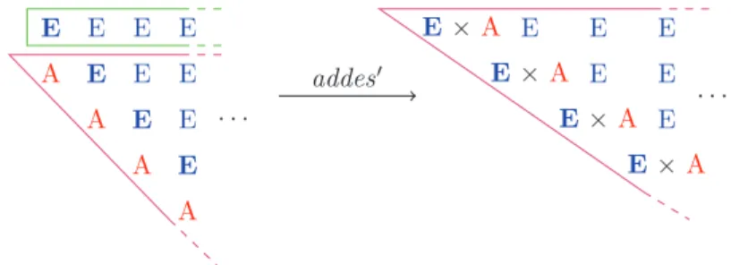
The definition of fromStreamRep is also quite intuitive. We have to construct the two elements that compose elements of type Tri. The top remains the top as before, this is again trivial. For the rest, we have to “glue” the first row to the rest of the triangle (basically the inverse of the cut and es_cut functions on Tri′
) before transforming it again. We call addes′
the function that performs this operation, as shown in Figure 9.
E E E E E E A A A A E E E E . . . E E E E E E E ×A E×A E×A E×A . . . addes′
Figure 9 Definition of addes′
◮Definition 20(addes′: ∀A. Str E → Tri′A→ Tri′(E × A), defined corecursively). addes′
(e :: es) t := éée, top′
tê, esê :: addes′
(frow′
t) (rest′ t)
◮Definition 21(fromStreamRep : ∀A. Tri′A→ Tri A, defined corecursively). fromStreamRep t:= constr (top′
t)!fromStreamRep (addes′
(frow′ t) (rest′
t))"
◮ Remark. Our first idea was to do the gluing after the transformation. Indeed, as the
transformation does not affect the elements of E, it seemed more natural to us not to submit this part to the corecursive call of the transformation. Thus, we wanted to define
fromStreamRep coinductively as follows:
fromStreamRep t:= constr (top′
t) (addes (frow′
t) (fromStreamRep (rest′ t)))
However, even if this seems harmless, this definition cannot be accepted by Coq since the corecursive call to fromStreamRep is not guarded (it is an argument of addes and not of a constructor). Nevertheless, we have shown that the solution to the previous equation is unique with respect to pointwise bisimilarity and that fromStreamRep of Definition 21 satisfies it.
◮Lemma 22. ∀A∀(t : Tri′A). toStreamRep (fromStreamRep t) ∼= t
Proof. To prove this result, we actually prove the following stronger result that we then only instantiate to finish the proof:
∀A∀(t : Tri′
A)(u : Tri A), toStreamRep (fromStreamRep t) ∼= u ⇒ t ∼= u
The proof of this statement is a simple coinduction, that uses some straightforward results on cut and addes′
. ◭
◮Lemma 23. ∀A∀(t : Tri A). fromStreamRep (toStreamRep t) ≃ t
Proof. We use the same technique as before. We prove a stronger result that we instiantiate to prove our lemma:
∀A∀(t : Tri A)(u : Tri′
A). fromStreamRep (toStreamRep t) ≃ u ⇒ t ≃ u
Here again, the proof is a straightforward coinduction using compatibility of top and rest with ≃ and a simple result on addes′
3.2
Redecoration on Tri
′Thus, we have a completely different view of the triangles, but still, it is fully equivalent to the original one. The interest of this view is that now the redecoration is very easy to perform. Indeed, before, the tricky part was that we had to lift the function f to trapeziums, and therefore to cut out the elements of E remaining (implicitly) from the first row. The problem was that we roughly had to cut out a row, while we were reasoning on columns. Here, as we directly reason on rows, it is much easier. As shown in Figure 10, the three elements of the transformed triangle will be:
the top is the application of f to the whole triangle (as before)
the first row of elements of E is the same row as in the original triangle (and as we said we have direct access to it)
the rest of the triangle is the application of the redecoration function to the rest
E E E E E E A A A A . . . E E E E E E B B B B . . . f redec′ f id
Figure 10 Definition of redecoration
Therefore, we can define the redecoration function for Tri′
as follows:
◮Definition 24(redec′ : ∀A∀B. (Tri′A→ B) → Tri′A→ Tri′B, defined corecursively). redec′
f t:= éf t, frow′
tê :: redec′ f(rest′
t)
We can finally show that this new version of the redecoration is equivalent to the previous one, modulo compatibility, using the conversion functions. We show that:
◮Lemma 25. ∀f, (∀t t′ , t ∼= t′ ⇒ f t = f t′ ) ⇒ ∀t, redec′
f t ∼= toStreamRep (redec (f ◦ toStreamRep) (fromStreamRep t))
◮Lemma 26.
∀f, (∀t t′ , t≃ t′
⇒ f t = f t′
)
⇒ ∀t, redec f t ≃ fromStreamRep (redec′
(f ◦ fromStreamRep) (toStreamRep t))
◮Remark. The compatibility hypotheses here are needed to work with Tri. Up to these
extra requirements, the two conversion functions yield an isomorphism of comonads (the associated properties for top and top′
are immediate by definition).
3.3
Simplifying redecoration again
As the representation of infinite triangles Tri′
is only as a stream of streams, we can use standard functions on streams to define redecoration. Indeed, redecoration can be interpreted
as consisting of applying a function to each element of the diagonal of an infinite triangle, where each element of the diagonal is itself a triangle (iterated tails of the given triangle). We can thus decompose the redecoration operation into two steps: first transform the infinite triangle into a triangle of triangles and then apply the transformation function on the elements of the diagonal, as shown in Figure 11.
E E E E E E A A A A . . . E E E E E E E A A A A . . . E E E A A A . . . E E E E E E A A . . . A. . . . . . E E E E E E B B B B . . . 1st step 2nd step
Figure 11 Idea of another definition of redecoration
◮Remark. Figure 11 is only a visualization of what happens, and has to be taken lightly. In
particular, all the elements of the diagonal of the middle triangle are infinite triangles, as we said. But, in order to visualize better what we do, their size seems to decrease since we cut out the first row of the previous element of the diagonal.
These two steps are then trivial to define on streams. Indeed, the first step consists of replacing all the elements of A by the corresponding iterated tail of the triangle itself. In fact, the information about the elements of E is redundant. Indeed, it is contained in the terms of the diagonal themselves (the row of elements of E “to the right” of an element of the diagonal is the first row of this element, minus the element of A). Therefore, we can omit them and only concentrate on the triangles. Thus, we need to obtain the stream of all the iterated tails of the initial triangle (see the first part of Figure 12). This is given by the classical tails operation defined below:
◮Definition 27(tails : ∀C. Str C → Str(Str C), viewed coinductively). tails s := s :: tails(tl s) ◮Remark. The function tails has the signature of the comultiplication operation in a comonad
based on Str according to the classical definition of comonads [8] (the term “comultiplication” is not used there, but only the letter δ that is dual to the multiplication of a monad). See Lemma 32 below for the constructive comonad based on Str.
In Figure 11, the second step only consists of applying f to all the elements of the diagonal. In fact, the first step corresponds to transforming t of type Tri′
Ainto
map!λx.éx, frow′
xê" (tails t) , and the second one consists in transforming s of type Tri′
(Tri′ A) into
map!λéu, esê. éf u, esê" s .
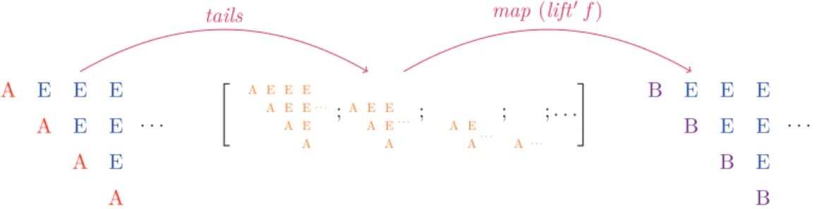
We can alternatively see the transformation of t into tails t as the first step, and the two successive map operations as the second step, which is therefore (by applying the functor law for map saying that map’s compose) performed by map (lift′
f), with lift′
defined as follows:
◮Definition 28(lift′: ∀A∀B. (Tri′A→ B) → Tri′A→ B × Str E). lift′
f := λx.éf x, frow′ xê
As for rest and rest′
, lift and lift′
are unrelated and belong to the respective point of view. This new version of the redecoration operation is shown in Figure 12.
E E E E E E A A A A . . . C D E A A A A . . . ; E E E A A A . . . ; E E E E E E A A. . . ; A. . . ; . . . E E E E E E B B B B . . .
tails map (lift′f)
Figure 12 Another definition of redecoration
Thus, we define a new version of the redecoration operation as follows:
◮Definition 29(redec′alt: ∀A∀B. (Tri′A→ B) → Tri′A→ Tri′B). redec′
altf t:= map (lift
′
f) (tails t)
One can then easily show that this operation is equivalent to the previous one:
◮Lemma 30. ∀A∀B∀(f : Tri′A→ B)∀(t : Tri′A). redec′f t≡ redecalt′ f t
The proof is a straightforward coinduction.
It is interesting to note that here, we do not need the bisimulation relation defined on
Tri′
. We can directly use the standard relation on Str, ≡. This should not be surprising. Indeed, here we only really manipulate streams. Those streams are made of pairs and we only manipulate the finite part of each pair (the first element). The second one is only a copy. Therefore the relation ∼= would be artificial here.
Let’s continue abstracting and define redec′
gen as follows:
◮Definition 31(redec′gen : ∀A∀B. (Str A → B) → Str A → Str B). redec′
genf s:= map f (tails s)
As we remarked previously, tails has the signature of a comultiplication for a comonad (in the triple format [8]) based on Str, and it is well known that map is the functor (on morphisms) for Str. Therefore, redec′
gen becomes the cobind operation of this comonad, generically. We
do not develop this piece of constructive category theory here, but only state the result for this instance:
◮Lemma 32. The type transformation Str, the projection function hd and redec′gen form a constructive comonad with respect to ≡.
This section is inspired by Adriano [2] who suggested a redecoration function for Haskell lists just in this form. More precisely, a function slide :: ([a] -> b) -> [a] -> [b] was defined by slide f = map f.tails. Note that Haskell lists can be finite and infinite, thus this definition captured streams as well.
The function redec′
alt is an instance of redec
′
gen, i. e., the following lemma is trivial:
Therefore, it is natural to show the three laws of comonads for redec′
alt and the proofs are
much simplified by the use of redec′
gen. In particular, we can show a kind of commutativity
of lift′
with redec′
alt.
◮Lemma 34. The type transformation Tri′, the projection function top′ and redecalt′ form a constructive comonad with respect to ≡ (more precisely, the equivalence relation is ≡A×Str E
for every A).
◮Remark. Through the functions toStreamRep and fromStreamRep, one can then transfer
this comonad structure back to Tri. Since Lemma 25 and Lemma 26 require compatibility of f with bisimilarity, this will not even give a constructive weak comonad, but the first and third law have to be relativized to compatible f ’s as well. Still, this does not seem a problematic constraint. Anyway, Lemma 11 has been proved independently of streams.
4
Conclusion
In this paper we have presented various verifications of the redecoration algorithm for infinite triangles. We have first dualized directly the representation for finite triangles by a nested inductive datatype to obtain a nested coinductive datatype. In both cases, the triangles are visualized by their columns. We have implemented the corresponding redecoration algorithm
redec (already available [1] in higher-order parametric polymorphism) and shown that we (only) obtained a constructive weak comonad (because of the compatibility hypothesis required). In this part, the redecoration algorithm, although deduced directly from the finite case, is quite tricky to manipulate because of the cutting and lifting it requires.
We then noticed that we could also consider the triangles by their rows, representing this time the triangles by purely coinductive datatypes, Tri′
, where we only took advantage of the existing type of streams (Str). This new visualization allowed us to define – keeping the same algorithmic idea as before – a function of redecoration redec′
already simpler than
redec and equivalent to it, modulo compatibility. But taking advantage of this representation by streams, we can simplify again the redecoration algorithm, using only standard functions on streams. This new function redec′
alt is fully equivalent to redec
′
. Generalizing again, we get nearly for free the cobind of the comonad Str, redec′
gen. This finally allows us to prove
the three comonad laws for redec′
alt.
In short, we have shown that the redecoration function, which is a quite subtle operation if we translate it directly from the finite triangles, reduces to something very basic in the completely infinite (i. e., in both directions) view of the infinite triangles. In this case, it is much easier to work with only infinite elements than with partially finite ones in the sense of consisting of infinitely many finitely presented columns. In fact, the stream representation is even easier to manipulate than the representation of finite triangles, and the comonad laws even hold with less restrictions due to constructivity.
Notice that the row-based view would not have given new insights for finite triangles. Indeed, as they are symmetric, we would have obtained exactly the same representation as for the column-based approach, only perceived with interchanged roles of rows and columns.
As a final remark on the Coq side, the improved support for setoid rewriting and the class mechanism [12] has shown to be of great help for the formalization and verification decribed in this paper.
References
1 Andreas Abel, Ralph Matthes, and Tarmo Uustalu. Iteration and coiteration schemes for higher-order and nested datatypes. Theoretical Computer Science, 333(1–2):3–66, 2005.
2 Jorge Adriano. Answer to Markus Schnell’s message slide: useful function? Haskell Mailing List, November 2002.
3 Yves Bertot and Pierre Castéran. Interactive Theorem Proving and Program Development.
Coq’Art: The Calculus of Inductive Constructions. Texts in Theoretical Computer Science.
Springer Verlag, 2004.
4 Richard Bird and Lambert Meertens. Nested datatypes. In Johan Jeuring, editor,
Math-ematics of Program Construction, MPC’98, Proceedings, volume 1422 of Lecture Notes in Computer Science, pages 52–67. Springer Verlag, 1998.
5 Richard Bird and Ross Paterson. Generalised folds for nested datatypes. Formal Aspects
of Computing, 11(2):200–222, 1999.
6 Nils Anders Danielsson. Beating the productivity checker using embedded languages. In Ana Bove, Ekaterina Komendantskaya, and Milad Niqui, editors, PAR, volume 43 of
EPTCS, pages 29–48, 2010.
7 Nils Anders Danielsson and Thorsten Altenkirch. Subtyping, declaratively. In Claude Bolduc, Jules Desharnais, and Béchir Ktari, editors, Mathematics of Program Construction, volume 6120 of Lecture Notes in Computer Science, pages 100–118. Springer, 2010.
8 Saunders Mac Lane. Categories for the Working Mathematician, volume 5 of Graduate
Texts in Mathematics. Springer Verlag, second edition, 1998.
9 Ralph Matthes and Celia Picard. Formalization in Coq for this article, 2012. www.irit. fr/~Celia.Picard/Coq/Redecoration/.
10 Ralph Matthes and Martin Strecker. Verification of the redecoration algorithm for tri-angular matrices. In Furio Honsell, Marino Miculan, and Ivan Scagnetto, editors, Types
for Proofs and Programs, International Conference, TYPES 2007, Revised Selected Papers,
volume 4941 of Lecture Notes in Computer Science, pages 125–141. Springer Verlag, 2008.
11 Celia Picard. Représentation coinductive des graphes. PhD thesis, Université de Toulouse, 2012.
12 Matthieu Sozeau and Nicolas Oury. First-class type classes. In Otmane Aït Mohamed, César Muñoz, and Sofiène Tahar, editors, TPHOLs, volume 5170 of Lecture Notes in Computer
Science, pages 278–293. Springer, 2008.
13 The Coq Development Team. The Coq Proof Assistant Reference Manual. INRIA.
14 Tarmo Uustalu and Varmo Vene. The dual of substitution is redecoration. In Kevin Ham-mond and Sharon Curtis, editors, Scottish Functional Programming Workshop, volume 3 of Trends in Functional Programming, pages 99–110. Intellect, 2001.