Methodological Issues of the Master Plan Schedule Construction in Mass Customization

22nd International Conference on Production Research

METHODOLOGICAL ISSUES OF THE MASTER PLAN SCHEDULE CONSTRUCTION IN

MASS CUSTOMIZATION

Abstract Id: SCML10356

LAMSADE, Université Paris-Dauphine, Place de Lattre de Tassigny F75775 Paris, France

Abstract

In global mass customization supply chains, the geographical dispersion of plants complicates flow control. Because of the high product diversity, the MPS of the final assembly lines is defined for Alternative Modules (AMs). Analysis of the visible diversity, through a car configurator, shows restrictions in the combinations of AMs. Choices made by the customer from the visible diversity trigger choices in the non-visible diversity. Causes and formal representations of the relations between AMs are analyzed. The MPS construction rests on commercial forecasts, for few sets of AMs, and on production information. Their combination leads to a typology that decreases the number of MPSs to build. These MPSs can be defined either through the use of completely defined products, which implies a deterministic view of the MPS construction, or the direct use of planning bills of materials, which offers the possibility of managing, on stochastic bases, the production beyond the frozen horizon.

Keywords

Alternative Modules, Planning Bill of Material, Mass customization, Diversity, Master Production Schedule, Product Configurator.

1 INTRODUCTION

Few companies have gone as far as those in the automobile industry in the application of mass customization. Even if the advantages for customers appear to be more or less obvious, the impacts of this strategy on the management of the Supply Chain’s production part are not as clear. This paper, which uses the automotive industry as an example, analyzes one of the impacts of this diversity.

From a production point of view, diversity is obtained in the assembly line through the combination of alternative (engines, gear boxes…) or optional (sunroof…) modules and through a few physical direct operations of differentiation (color…). Usually, customers are not aware of the whole diversity (alternator…).

This diversity has several consequences in the production process. By influencing the products’ design (modular design, sharing of platforms and components between different ranges of products), it determines the design and the capacity of the assembly line that must be able to support a certain diversity, even if it occasionally causes variability of operation time on some stations, which creates problems in sequencing orders. This sequencing leads to parts requirements for each station, which are necessarily more complicated for alternative modules. Within a longer time frame, diversity poses a problem of replenishment management in the Supply Chain’s productive part, which is pulled by the assembly line.

This paper addresses this last problem. Scheduling a lightly diversified production may be accomplished at the end-product level, as the limited number of end products allows the determination of a Master Production Schedule (MPS) from their corresponding demand forecasts. In production with mass customization, the variety of final products prevents a direct forecast at the level of the finished goods; demand forecasting is only possible at a more aggregate level, i.e., at the level of the alternative modules. This involves some methodological issues that will be analyzed in this paper.

It is necessary to properly describe this diversity (section 2), which has an impact on the available information (section 3) that can be used to schedule the production of

alternative modules and their required components with one of two possible approaches (section 4).

2 DIVERSITY ANALYSIS

The diversity that is observed by a person who is considering purchasing a car is presented by the configurator of the brand (defined below); this diversity allows him to explicitly choose the AMs that are valuable to him. The customer who goes directly to a car dealer will be implicitly guided in his choices the same way. This apparent diversity is only a part of the diversity offered. First, it is important to distinguish the visible from the non-visible diversity (§2.1). Then, types of restrictions that ban the free combinations of AMs have to be clarified before introducing formal representations that describe those restrictions (§2.2).

2.1 Visible and non-visible diversity

A configurator is a web tool for customers that permits them to not only interactively define the end-product in accordance with their desires, but also to do so in a progressive manner because the choices they make at a certain point could be constrained by previous choices. For example, the configurator for T model1 usually orders the choices in this manner, but the order is not rigidly enforced: a level of the equipment, an engine and a gear box, plus various options (color, alloy wheels, air conditioning, parking sensors…). The equipment level indicates the level of complexity of services provided and plays a specific role in the determination of some AMs that are non-visible for customers; the concept of equipment level will be developed later.

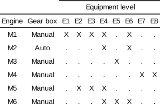
Visible diversity present in the T model’s French configurator leads to a commercial offer that provides eight equipment levels, six engines, eleven colors, fifteen wheel rims and over fifty possible options. The actual diversity is not the product of cardinality of those sets as presented in [4]; in fact, the combinations that are permitted are highly limited. The following table, which is an extraction of

1 _{In order to respect confidentiality this paper uses generic names}

for products and brands

illustrates these restrictions. Stablein et al. [9] propose a formula to measure the diversity offered while taking into account the constraints between AMs.

Table 1: Example of the limitation of diversity

Engine Gear box E1 E2 E3 E4 E5 E6 E7 E8 M1 Manual X X X X . X . . M2 Auto . . . X . X . . M3 Manual . . . . X . . . M4 Manual . . . X X M5 Manual . X X X . . . . M6 Manual . . . X X X . . Equipment level

At this point, AMs should be defined. An AM is a component chosen from an Alternative Modules Set (AMS), a group of AMs in which all members have the same set of functions. AMs of a single AMS are assembled in the same station of the line. Optional components (sunroof, parking sensors, embedded computer…) are particular cases of an AM in which, implicitly, the alternative of the optional module may be a physical object (sheet metal roof, bumper without sensors…) or nothing at all (absence of the embedded computer…); in both cases, from a descriptive point of view and to stay general, it is possible to introduce a fictive AM representing the non-use of an optional module. Physical, direct operations of differentiation, such as color, are not included because they do not have consequences on the upstream part of the Supply Chain.

The definitions of AMs and AMSs proposed above are only applicable to physical objects. They must be extended to permit the description of the production variety as it is on an assembly line; this requires three generalizations: ● The equipment level can be regarded as an AMS,

because a vehicle can only be associated with a single equipment level but it is virtual. Its function is two-fold: it limits, for technical and/or commercial reasons, combinations of AMs that belong to different AMSs (this is what the above table illustrates), and it determines the AMs of some other AMSs, some of which are visible and some of which are not. This point will be developed further.

● The commercial offer for the same range of vehicle changes from region to region. “Region” refers to a set of countries grouped by a same commercial offer that is described in a dedicated configurator. Often, all the offers overlap, but each region can offer some specific AM for commercial or regulatory reasons. For example, English drivers want the driver’s side to be on the right, German pollution standards are stricter than French standards, the canvas roof is only available in Germany, and the smoker pack is only available in the United Kingdom. Generally, an assembly line produces vehicles for different markets. The AMSs used in the description of vehicles that can be produced on a line merge the AM lists that are associated with different regions; for example, the AMS “T model’s roof” must include the AMs “sheet metal roof”, “sun roof” and “canvas roof”, which results from the consolidation of German and French AMSs. ● The characteristics of the offer evolve with time for

three reasons. First, some problematic components may be replaced. Then, range rejuvenating can lead

combinations between AMSs can evolve with time. For example, it may be decided that, for a certain period and equipment level, an optional air conditioning system should become standard. Therefore the diversity offered by a region is always a dated picture that is usable until a new change. This change in time is identified in the literature by the concept of dynamic diversity (Pil & Holweg, [7]). In the following, these temporal aspects will not be taken into account. Later, the implications of the possibility of producing vehicles of different ranges (T and C models for example) in the same assembly line will be introduced. This is not a variety of the commercial offer but a variety of production, which complicates control of replenishments of the line if the production sharing between ranges is not stable. In addition to the visible diversity, there is diversity that is not visible by customers.

Without being aware of it, the customer implicitly and progressively determines many AMs through choices in the configurator, especially by selecting the equipment level. For example, the equipment level AMS not only determines certain visible components (interior plastic quality, shape of the seat…), but also, most importantly, many non-visible AMs that are not shown in the configurator, such as wiring kits or alternators that are linked with the selected electric equipment (air conditioning system, sunroof’s engine, electrical outside mirror or electric window…). These restrictions result from taking into account the constraints based on technical aspects (geometric, electric…) and commercial aspects (segmentations that permit a coherence of the offer and limit cannibalization effects between ranges). The examination of those constraints is a necessary first step for the analysis of their formulations.

2.2 Analysis and formal representation of relations between AMs

Three types of relations between AMs (and thus between AMSs) can be identified.

● Total independency with no restrictions; for example, parking sensors can be assembled on any T-model. ● With an injective relation, the choice of an AM in an

AMS that is visible in the configurator implies the choice of an AM in another AMS that may or may not be visible, although the reverse is not true. For example, the choice of equipment level influences the choice of the electric wiring kit required by the vehicle. ● Compared to the previous relation, the bijective

relation is symmetric. An example is the M2 engine, which requires the use of the automatic gear box that is only compatible with that particular engine.

● In the “conjunctive” relation, the choice of a combination of AMs in different AMSs determines or limits the choice of an AM in another AMS. This can be illustrated by the choice of air conditioning system, which depends on the equipment level: the system is not permitted for the lowest equipment levels, is optional for mid-range equipment levels and is standard for higher ranges of equipment levels. The vehicle resulting from these constraints is technically coherent. These constraints can be taken into account only if they are transcribed in the Information System. The next paragraphs will examine how to transcribe the constraints. In the formalism of relational databases, AMs are grouped into entity types, and each AM is associated with a unique AMS that belongs to the AMS entity type. The analysis of the dependency relations identified above leads to first introducing an “is-a” relationship and the notion of role in

22nd International Conference on Production Research

order to realize functional dependency between two AMs in the case of injective relations (as it is usually done in the description of the relationship that links an “incuding component” with an “included” component). The bijective relation can be solved the same way. Conjunctive relations can be managed with an association type whose key is a concatenation of the keys of AMs that belong to different AMSs; this association leads to a functional dependency that points to a unique AM of a different AMS, or to a multivalued dependency if it concerns a sub-set of AMs that belongs to the other AMS. The possibility that the AMS belongs to several different associations poses the problem of the combination of AMs, which may lead to semantics errors, as in the problem regarding the fifth normal form of the relational databases. In practice, without general rules it is better to take into account integrity constraints through associations that respect the fifth normal form. However, the keys for the different associations that result from taking these constraints into account may be too long for practical use.

Bertrand & al. [2] had investigated solutions for this problem of formally representing those integrity constraints using the concept of pseudo-items, defined as a group of interdependent AMSs, to obtain an independency between items (pseudo or not). Searching the independency between all items leads to pseudo-items that are composed of almost all of the items; thus, this approach is not as effective as is needed in the car industry.

A second approach can be used to formalize those relations. Based on Knowledge Engineering, it calls for predicates to describe conditions of requirement of the AMs that belong to non-independent AMSs. For example, let’s introduce three AMSs

{ }

{ }

{ }

i

A , B_i and C_i to be their respective AMs. If C₇ is mandatory when A₁ and B₁are used or if A₁ and B₂are assembled, it is possible to represent the predicate, denoted C_i−1, that describes the condition of requirement of the C_i module: C₇−1=A₁∧(B₁∨B₂). This predicate is a reverse Bill of Material and is similar to the pegging approach that is well-known in MRP use. Even if this method to describe restrictions is correct, it is very difficult to use in the studied context because of the length of predicates.

These two approaches allow the handling of integrity constraints due to commercial offer restrictions. They are fully usable only at the car level by defining the envelope of the authorized combinations. As explained later, the planning process must use the concept of the Planning Bill of Material (PBOM), which is determined by the structure of MAs observed in a set of vehicles produced previously or to be produced in the near future.

3 INPUT INFORMATION AVAILABLE FOR PLANNING

As explained previously, production planning cannot be based on commercial forecasts expressed at the products level because of the too large variety of end-products. Thus, it must be based on forecasts at the EMAs level or at a combination of EMAs level (§3.1.). This information must be combined with production information about the BOM and some Supply Chain characteristics (3.2.). Combining commercial forecast characteristics and production information leads to the definition of an AMs typology that makes it possible to define an MPS for a decreased number of AMSs (§3.3).

3.1 Commercial forecasts

Sales management, after first agreeing with production management, gives its forecasts in terms of the volume of production for an assembly line and for a period. Then, it states, for the same period, forecast structures of demand that can be regarded as forecasts of the Planning Bill of Material (PBOM). These forecasts only address certain visible AMSs that are considered to be important for customers (practical or emotional value) or for manufacturers (because of value of modules and depth of the Supply Chain used). They take into account trends in the evolution of demand, the launching of new models on the market and the impact of special marketing practices of the manufacturer or its competitors (limited series, special offers…). The forecasts are assumed to respect integrity constraints between AMs considered in the analyses. For other AMSs, which are much more numerous, only historical data and information about the integrity constraints are available to create the corresponding MPS.

3.2 Production information

Usually, requirements of a highly diversified production, for the middle term calls for a PBOM, whose usage is not evident in the studied context (A). Taking into account certain Supply Chain characteristics limits the necessity of precise planning (B).

A. Planning Bill of Material

PBOMs are used in MRP to solve problems with alternative modules that require components with a lead time longer than the frozen period. This method is based on the use of a generic BOM, which associates each AMS to a virtual component that points to the list of AMs that it includes; this association has a BOM coefficient that represents the demand part of the AM in the considered AMS. If constraints between AMSs exist, the PBOM cannot be used directly without care.

Four remarks should be stated about the determination of the PBOM coefficients:

● PBOMs do not take into account integrity constraints that are defined at the vehicle level (as explained at the end of §2.2). However, the BOM coefficients must respect some numerical constraints resulting from the indirect accounting of those integrity constraints. For example, if the choice of the M_i engine implies the use of the GB_j gear box, the BOM coefficient for GB_j

cannot be lower than the M_icoefficient.

● The PBOM is defined for interchangeable lines (or a set of interchangeable line in a factory) because it depends on the satisfied demand structure. If the same line has to supply the demands of different regions, as it was stated in §2.1, it is better to use consolidated AMSs. Therefore, the PBOM coefficients to be used for an aggregated AMS are necessarily defined for an AMS whose AMs are the merge of all of the AMSs lists of each region (§2.1) and whose coefficients are the weighted sum of the regional BOM coefficients multiplied by the part of the region in the whole production.

● The same production line could assemble vehicles belonging to different ranges (T model and C model) if those vehicles share the same platform and many components. Thus, a station of the line may assemble AMs belonging to two AMSs associated with two ranges, as long as both AMSs have the same main function or share some MAs. If the share of production between the two ranges is stable, those coefficients are easily determined by using the method explained

problem is more difficult, and the PBOM defined for each range has to be conserved in order to be subsequently used in conjunction with a production-sharing ratio between the two ranges. These hypotheses can be determinist or stochastic (in this case, the Monte Carlo method must be used to determine the random demand of an AM). In addition, in this case of a random share between two ranges, the demand of assembled systematic components that are not used by the two ranges becomes random. In this paper, only the case of a line dedicated to a single model or with a constant share between two ranges will be considered.

● Postponement decisions are strategic; they bind short- and middle-term decisions as planning ones. Their impacts on the definition of the PBOM are substantial. The engine factory can send to the assembly line engines that are customized and already include the alternator chosen for the required electrical power and filters that depend on the regulations of the country where the car is sold. It is also possible for the engine factory to deliver “bare” engines to the assembly factory, which is now responsible for assembling the components of the engine differentiation. In this case, the engine BOM is reduced and the assembly factory has to acquire its supplies of alternators, filters… It increases the number of AMSs managed by the assembly factory and, thus, the BOM length. In order to illustrate this idea, for the T-model, there are four “bare” engines and thirty eight customized engines. If postponement is impossible, it is better if the engine factory defines the “bare” engine, which is a transient stage in the process (it cannot be stocked), as a phantom component in the BOM in order to use the more reliable forecasts that exist at the “bare” engine level.

B. Supply Chain characteristics

Requirements’ control of the AMs assembled on a line does not automatically involve the use of a MPS for each AM. Taking into account the Order Penetration Point (OPP) and characteristics about the cost and bulk of the AM bulk can lead to certain AMs being excluded from the planning process.

The supply of the assembly line is always the result of previous purchase orders that had been taken to a tier one supplier. The vendor’s production is called “build to order” if it aims to fulfill a certain demand that is known only from the ordering date and is regarded as “build to stock” in the opposite case. Build to order can be managed by a synchronized supply that often involves an assemble-to-order configuration (seat’s supply, for example) or a synchronized production (for example, bumpers’ production, if the vendor is near assembly line).

The OPP defines both the frozen period, during which production orders are known and cannot be modified, and the lead-time, which is the time between the purchase order date and the delivery date. The supplier necessarily produces with a build to stock configuration if its lead time is longer than its customer’s OPP. A tier one vendor often has many customers (even if it belongs to the same company because it may deliver to plants dispersed all over the world; for example, this is the case of engine factories); therefore, it usually simultaneously builds to order and to stock.

Purchase orders that can be fulfilled by build to order production may not need the knowledge of precise requirements and be controlled by a periodic order-up-to level policy or by an ordering point inventory model. This

and bulk, of packaging constraints and of global cost of stock and data processing. A lot of AMs (stickers, outside mirrors’ hulls…) can fall into this category.

3.3 AMs typology usable for differentiate requirements’ management

The mix of commercial and production information leads to suggest an AMs typology that reduces the scope of requirements planning and, thus, limits the number of AMs MPS needed.

Within this framework, it is necessary to reintegrate all the assembled systematic components whose demand only depends on the production’s total volume forecasted by the sales management. Then, the following should be distinguished:

● Independent AMs that are directly steered by sales management forecasts or those considered to be equivalent because of their relative independency from the sales forecast.

● AMs whose demand is deduced from independent AMs. These AMs could be visible (in the configurator) or not.

This information could be combined with information deduced from the OPP and with information about certain SC characteristics to potentially isolate AMs whose requirements management could be autonomous.

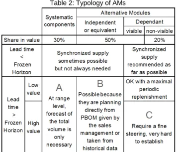
The average shares in value of the assembled components on the production line that are in the following table have been observed for the T-model.

Table 2: Typology of AMs

The definition of the MPS, necessary a priori for all AMs, can be restricted to subsets B and C, with harder methodological difficulties for subset C. The subset concerned with autonomous management must use an inventory model that limits the shortage to an acceptable level, while considering the imprecision of the parameters used.

4 POSSIBLE MECHANISMS FOR ALTERNATIVE

MODULES PLANNING

Starting from the double observation that AMs do not combine freely and that sales management forecasts are made only for certain AMSs, it is obvious that the construction of the MPS for other AMSs poses a real methodological problem. This is true even if the problem is narrowed to AMSs whose lead time is longer than the frozen period. Two solution methods are possible. The first consists in transforming sales management forecasts to

22nd International Conference on Production Research

forecasts on the Completely Defined end-Products (CDP) that are in accordance with the integrity constraints of the relations between AMs in order to construct an MPS for each AM (§4.1.). The second method consists of directly using PBOMs, with some precautions (§4.2.).

4.1 CDP use

With respect to the technical and the commercial dated constraints, a CDP is one of the possible combinations of AMs that represents all of the AMSs, excluding certain accessories of personalization (stickers, roof rails...) that are deemed irrelevant for the supply management. A CDP has no physical existence, but it is the reflection of what could be a real finished product; it may be qualified as a virtual product. By construction, a CDP meets all of the constraints imposed by engineering (technical constraints) and sales management (business constraints). This property gives to the CDP the same consistency as the products that are actually sold.

The coherence properties and the tangibility of the CDP are reassuring for supply chain managers. Their use for middle-term planning is seen as a simple extension of short-term scheduling. The use of a CDP guarantees consistent component requisitions under the product nomenclature through the use of inverse nomenclatures. If the use of CDP is essential for short-term scheduling, a planning with CDP beyond the frozen horizon gives the illusion of dealing with a certain forecasted production. Unfortunately, the stability conditions are not met in the middle-term. Changes in production programs with rolling planning cause disturbances that generate a bullwhip effect in the upstream-supply chain (see Childerhouse et

al. [3] and Niranjan et al. [6]). The instability of production

programs, without affecting systematically used components (set A), generates a loss of effectiveness and efficiency in the supply management of components of sets B and C.

The information provided by the sales department, in the form of demand forecast patterns on certain AMs (similar to PBOMs), is insufficient to allow supply management for the components of set C. In fact, the use of the components of set C in the assembly line depends on the partial or the finished product configuration. The principle of CDP planning is desegregating the sales department demand by progressively combining the AMs that are directly covered by the PBOMs. The combination of AMs of set B enables the identification of the induced AMs for which there is no initial information. The desegregation of the commercial demand for constructing a CDP is completed in each period of the planning horizon under a strict compliance with the technical and the business dated constraints. The MPS that is described at the zero level of nomenclature is then exploited in a classical MRP calculation.

While seeking strict consistency within the meaning of the product nomenclature, CDP planning is not without consequences on the performance of the upstream supply chain. Inherent rules within the desegregating process of the sales demand can cause serious disturbances, which propagate along the upstream supply chain. These disturbances, which ultimately have similar consequences on the flow control beyond the frozen horizon, are twofold.

- Sales demand deformation: If the successive steps of the sales demand desegregating process contribute to distort the initial demand, i.e., the baseline information on future demand, this can generate a production schedule that is inconsistent with production orders reassembled by the commercial network. A modification of the MPS is necessary, triggering a vicious circle described by Childerhouse

et al. [3]. Sales demand deformation is a "static"

distortion observed at time t for the same period of the planning horizon.

- Rolling planning instability: It happens when the production program that is generated at different execution cycles of the desegregating process exhibits large differences despite a stable sales demand. Rolling planning instability generates difficulties to suppliers. This "dynamic" distortion is bound to the periodic use of the sales demand desegregating process.

The analysis of the sales demand desegregating process for the CDP planning in a European car manufacturer has revealed the existence of the two phenomena described above. Starting from PBOMs provided by the sales department on a limited number of AMs, the solution adopted by the manufacturer to generate CDP planning is the use of mathematical programming methods to solve a series of optimization problems for each planning period. Two properties, inherent to the problem of CDP generation, are causing the deformation of the sales demand and the rolling planning instability.

- As illustrated in table 2, two coherent planning BOMs at the Equipment Level and Engine are not sufficient to derive average utilization rates for the Equipment Level / Engine combination. We face an underdetermined mathematical problem with, for this example, 14 equations (number of AMs with a planning bill known) and 16 unknowns (number of possible combinations). To be solved, this problem is transformed into a tradeoff between the planning BOMs compliance (marginal sums) and the forecast rates’ proximity to permissible combinations (these rates are generally derived from historical data). This arbitration is intended to distort the coefficients of the PBOM because the strict respect of the sales demand is not a constraint.

- In a rolling planning, the robustness of the CDP generating process is measured according to its ability to provide a stable result from one planning cycle to another. The higher the sensitivity to changes of the sales demand desegregating process, the greater planning instability. A small change of input data causes increased nervousness in the MPS.

4.2 Direct use of PBOM

This section will deal neither with the planning of the component systematically used, nor with the planning of alternative modules in a made to stock configuration. For other AMSs and beyond the frozen period, the MPSs are defined by a direct exploitation of PBOMs without using the determinist vision of CDP. The demand of those AMs is considered random and the requirements’ control is based on a periodic replenishment. The AMS PBOMs coefficients are used as requisition probabilities of different AMs of the AMS and, for a given AMS, the daily need of the AMs follows a multinomial distribution. Two cases must be distinguished.

For the AMs in group B, for which sales department gives forecasts, the requirement’s control of the AMs - and of the components they require - does not pose a problem, as an extension of the MRP approach permits either a make to order or a make to stock configuration to be used to manage the affected upstream part of the Supply Chain (Giard & Sali, [5]). Different benchmarks used to test this approach in comparison to the CDP approach show relevant gains in efficiency (safety stocks reduction) and effectiveness (stock-out reduction).

for group B is difficult. Here, even if the above approach were still coherent to use, the problem is to define which PBOMs to use. It seems possible that if the forecast structural characteristics given by sales department are similar with those observed in the past, it is possible to use a PBOM defined from recent historical data. On the contrary, different solutions are possible:

- The simplest one consists in uprating a PBOM coefficient (used as probability); the limit is that it is impossible to know if the rating is sufficient (with an excessive shortage risk) or too high (with a useless safety stock level). If the value of the concerned AMs is not too high, this solution may be used with sufficient ratings.

- Another possible solution consists in using historical data and optimal multiple linear regression techniques to find relations between one deduced coefficient of an AM and the coefficients of potential AM inductors whose sales management forecasts are known. Benchmark studies between this approach and the CDP approach, conducted with approximately ten AMs used on the T-model, show a relevant superiority of this approach in both effectiveness and efficiency. Complementary comparative analyses must be completed in order to test the robustness of the proposed solutions to establish an MPS of the AMs of group C.

5 CONCLUSION

Requirements’ control of enterprises oriented in mass customization is improvable and investigations must be conducted in the framework of the approach of the direct use of PBOM.

To succeed in providing a correct offer to the market, the enterprises protect them with a considerable safety stock or by recurring emergency transport solutions. Those actions are in a curative way that is based too often, in arbitrages made, on local data that is disconnected from the initial sales forecasts. The improvement of requirements’ control, the object of this article, is a matter of preventive logic that uses the best forecasting information and lessens the importance of curative approaches.

The problem analysis is more complicated when an assembly line is shared by different products ranges whose daily production is not well known in advance. It is possible to use a revisable hypothesis about this sharing to establish MPSs. Within the framework of the second solution analyzed above, it is possible to combine this source of hazard with those already taken into account using the Monte Carlo method. Thus, the demand of systematic components used by only one product range becomes random. This increase of complexity militate in favor of an anticipation of the production partition rates between products ranges.

In practice, numerous methodological problems to efficiently steer requirements of a plant dedicated to mass customization have not yet been solved.

6 REFERENCES

[1] Anderson, D. M., Pine II, J., 1997. Agile Product

Development for Mass Customization: How to Develop and Deliver Products for Mass Customization, Niche Markets, JIT, Build-to-Order and Flexible Manufacturing, McGraw-Hill.

[2] Bertrand, J.W.M., Zuijderwijk, M and Hegge, H.M.H., 2000. Using hierarchical pseudo bills of material for customer order acceptance and optimal material replenishment in assemble to order manufacturing of

Production Economics, 66 (2) 171-184.

[3] Childerhouse, P., Disney, S.M. and Towill, D.R. (2008) On the impact of order volatility in the European automotive sector, International Journal of Production Economics, 114 (1) 2-13.

[4] Fisher, M.L. and Ittner, C.D., 1999. The Impact of Product Variety on Automobile Assembly Operations: Empirical Evidence and Simulation Analysis,

Management Science, 45 (6) 771-786.

[5] Giard, V. and Sali, M., 2012. Pilotage d’une chaîne logistique par une approche de type MRP dans un environnement partiellement aléatoire, Journal

Européen des Systèmes Automatisés (APII-JESA),

46 (1) 73-102.

[6] Niranjan, T.T., Wagner, S.M. et Aggarwal, V. 2011, Measuring information distortion in real-world supply chains, International Journal of Production Research, 49 (11) 3343 - 3362.

[7] Pil, F.K. et Holweg, M., 2004, Linking Product Variety to Order-Fulfillment Strategies, Interfaces, 35 (5) 394 - 403.

[8] Stablein, T., Holweg, M. et Miemczyk, J., 2011, Theoretical versus actual product variety: how much customisation do customers really demand?, International Journal of Operations & Production

Management, 31 (3) 350 - 370.

[9] Vollmann, T.E., Berry, W.L., and Whybark, D.C. 1997. Manufacturing planning and control systems. 4th ed., New York: Irwin/McGraw-Hill.