Multicriteria Evaluation-Based Conceptual
Framework for Composite Web Service Selection
Salem Chakhar1, Serge Haddad2, Lynda Mokdad1, Vincent Mousseau3, and
Samir Youcef1
1 LAMSADE, Universit´e Paris-Dauphine
Place du Mar´echal de Lattre de Tassigny, 75775 Paris Cedex 16, France
{salem.chakhar,mokdad,samir.youcef}@lamsade.dauphine.fr
2 Laboratoire Sp´ecification et V´erification, ´Ecole Normale Sup´erieure de Cachan
61, Avenue du Pr´esident Wilson 94235 Cachan Cedex, France [email protected]
3 Laboratoire G´enie Industriel, ´Ecole Centrale Paris
Grande Voie des Vignes, 92295 Chˆatenay-Malabry Cedex, France [email protected]
Abstract. The paper proposes a general framework to composite Web services selection based on multicriteria evaluation. The proposed frame-work extends the conventional Web services architecture by adding, in the registry, a new Multicriteria Evaluation Component (MEC) devoted to multicriteria evaluation. This additional component takes as input a set of composite Web services and a set of evaluation criteria and gen-erates a set of recommended composite Web services. In addition to the description of the conceptual architecture of the formwork, the paper also proposes solutions to construct and evaluate composite web services.
Keywords: Web service, Quality of Service, Multicriteria evaluation,
Web service composition, Web service selection, Performance evaluation
1
Introduction
Individual web services are conceptually limited to relatively simple function-alities modeled through a collection of simple operations. However, for certain types of applications, it is necessary to combine a set of individual Web services to obtain more complex ones, called composite or aggregated Web services. One important issue within Web service composition is related to the selection of the most appropriate one among the different possible compositions. One pos-sible solution is to use quality of service (QoS) to evaluate, compare and select the most appropriate composition(s). The QoS is defined as a combination of the different attributes of the Web services such as availability, response time, throughput, etc. The QoS is an important element of Web services and other modern technologies. Currently, most of works use successive evaluation of dif-ferent, non functional, aspects in order to attribute a general “level of quality”
to different composite Web services and to select the “best” one from these ser-vices. In these works, the evaluation of composite Web services is based either on a single evaluation criterion or, at best, on a weighted sum of several quantita-tive evaluation criteria. Both evaluation schemas are not appropriate in practice since: (i) a single criterion does not permit to encompass all the facets of the problem, (ii) weighted sum-like aggregation rules may lead to the compensation problem since worst evaluations can be compensated by higher evaluations, and (iii) several QoS evaluation criteria are naturally qualitative ones but weighted sum-like aggregation rules cannot deal with this type of evaluation criteria.
The goal of this research is to propose a general framework to composite Web services selection based on multicriteria evaluation. The proposed framework ex-tends the conventional Web services architecture by adding, in the registry, a new Multicriteria Evaluation Component (MEC) devoted to multicriteria evalu-ation. This additional component takes as input a set of composite Web services and a set of evaluation criteria. The output is a set of recommended compos-ite Web services. The paper also proposes a solution to generate the different potential compositions which will be the main input for the MEC. Further, the paper shows how composite web services can be evaluated.
Two types of compositions are generally distinguished: static and dynamic. Static composition supposes that all Web services are predefined and that the composition graph (see Section 7) cannot change during execution. With dy-namic composition, in turn, Web services are not predefined and composition graph may evolve over time. The dynamic composition is an important research issue. However, in this paper we assume a static composition environnement. The extension to dynamic composition is under investigation.
The paper is organized as follows. Section 2 presents some related work. Section 3 introduces the notion of quality of service (QoS). Section 4 details the architecture of the proposed framework. Sections 5 and 6 further detail MEC and W-IRIS. The latter is a special kind of Web service used by MEC to infer the preference parameters needed to apply the multicriteria classification method—which is ELECTRE TRI in this paper. Section 7 shows how the set of potential composite Web services is constructed. Section 8 discusses the problem of composite Web service evaluation. Section 9 gives an illustrative application. Section 10 discuses some computational issues. Section 11 concludes the paper.
2
Related work
As underlined in the introduction, to choose among the different possible com-positions, most of previous works use either a single QoS evaluation criterion or a weighted-sum of serval quantitative QoS evaluation criteria. The following are some examples. The author in [14] considers two evaluation criteria (time and cost) and assigns to each one a weight between 0 and 1. The single combined score is computed as a weighted average of the scores of all attributes. The best composition of Web services can then be decided on the basis of the optimum
combined score. One important limitation of this proposal is the compensation problem mentioned earlier.
In [7], the service definition models the concept of “placeholder activity” to cater for dynamic composition of Web services. A placeholder activity is an abstract activity replaced on the fly with an effective activity. The author in [3] deals with dynamic service selection based on user requirement expressed in terms of a query language. In [8], the author considers the problem of dynami-cally selecting several alternative tasks within workflow using QoS evaluation. In [1], the service selection is performed locally based on a selection policy involving the parameters of the request, the characteristic of the services, the history of past executions and the status of the ongoing executions. One important short-coming of [7][3][8][1] is the use of local selection strategy. In other terms, services are considered as independent. Within this strategy, there is no guarantee that the selected Web service is the best one.
To avoid the problem of sequential selection, Zeng et al. [23] propose the use of linear programming techniques to compute the “optimal” execution plans for composite Web service. However, the multi-attribute decision making approach used by the authors has the same limitation as weighted-sum aggregation rules, i.e., the compensation problem.
Maximilien and Singh [13] propose an ontology-based framework for dynamic Web service selection. However, they consider only a single criterion, which is not enough to take into account all the facets of the problem.
Menasc´e and Dubey [15] extends the work of Menasc´e et al. [16] on QoS bro-kering for service-oriented architectures (SOA) by designing, implementing, and experimentally evaluating a service selection QoS broker that maximizes a util-ity function for service consumers. These functions allow stakeholders to ascribe a value to the usefulness of a system as a function of several QoS criteria such as response time, throughput, and availability. This framework is very demand-ing in terms of preference information from the consumers. Indeed, consumer should provide to a QoS broker their utility functions and their cost constraints on the requested services. However, the most limitation of this work is the use of weighted-sum like optimization criterion, leading to compensation problem as mentioned earlier. One important finding of this paper is the use, by the QoS broker, of analytic queuing models to predict the QoS values of the various services that could be selected under varying workload conditions.
More recently, [10] use genetic algorithm for Web service selection with global QoS constraints. The authors integrate two policies (an enhanced initial policy and an evolution policy), which permits to overcome several shortcomings of genetic algorithm. The simulation on Web service selection shown an improved convergence and stability of genetic algorithm.
3
QoS evaluation criteria
Web services attributes can be organized into two families: functional require-ments and non functional requirerequire-ments (NFRs). To evaluate the NFRs of a
sys-tem, several works have used the notion of QoS. Different definitions to the QoS have been proposed. Schmidt et al. [20] define QoS as the set of “all properties other than the functional behavior of an application”. In the most general case, this term refers to a set of requirements wished (or imposed) by a user (human being or software component) to the performance of an application during its execution [12].
There are several QoS evaluation criteria. A comprehensive list of commonly used criteria is given in Table 1. For each criterion, we provide a brief description, the type (quantitative or qualitative), and the preference direction where max means “the higher, the better” and min means “the lower, the better”.
As mentioned by [14], the exact definition and measurement process for each criterion must be well-defined to give service consumers and providers a com-mon understanding. For ordinal QoS evaluation criteria, an ordinal measure-ment scale should be defined. A commonly used ordinal measuremeasure-ment scale is the Likert-type [21] one, which contains approximately equal number of favor-able and unfavorfavor-able levels. An example is the five-points scale: very low, low,
average, high, very high. These levels express difference in degrees but not
quan-tities. The authorized mathematical operations on an ordinal scale are: “equal to” (=), “less than” (<), and “more than” (>).
Interval or ratio measurement scales need to be defined for quantitative QoS evaluation criteria. There are not generally accepted formula to measure Web services on quantitative QoS evaluation criteria. Response time, for example, could be measured as an average over the past 15 minutes, as a 90th percentile, or as an array of average times for each 15-minute interval during the day [14].
Klingemann et al. [9] use a continuous-time Markov chain to estimate the response time and the cost of a workflow.
In [2], the author discusses four QoS evaluation criteria (response-time, cost, reliability and fidelity) and proposes different ways to use them to evaluative composite web services.
Maximilien and Singh [13] proposed an ontology-based framework for dy-namic Web service selection that provides a starting point for a QoS lingua franca. However, they did not address the fact that some QoS metrics, such as response time, depend on workload intensity level, which means a single value is not appropriate [14].
Youcef et al. [22] propose a simulation-based response-time evaluation.
4
Extended Web service architecture
We first present the conventional Web service architecture. Then, we introduce the proposed architecture. Next, we detail the different XML schema for in-formation exchange among the entities involved in the extended Web service model.
Name Description Type Preference Availability The degree to which a system, subsystem, or
equipment is operable and in a committable state at the start of a mission, when the mission is called for at an unknown, i.e., a random, time. In others terms, availability is the proportion of time a system is functional.
Quantitative max
Response time The lap of time from request sending to response reception.
Quantitative min Throughput The rate at witch a service can process requests. Quantitative max Reliability The likelihood of success using a service. Quantitative max Security It captures the level and kind of security a service
provides.
Qualitative max Robustness The degree to which a system or component can
function correctly in the presence of invalid in-puts or stressful environment conditions.
Qualitative max Scalability It defines whether the service capacities can be
increased as needed.
Qualitative max Integrity The quality aspect of how the Web service
main-tains the correctness of the interaction in respect to the source. Proper execution of Web service transactions will provide the correctness of inter-action. A transaction refers to a sequence of ac-tivities to be treated as a single unit of work. All the activities have to be completed to make the transaction successful. When a transaction does not complete, all the changes made are rolled back.
Qualitative max
Reputation It is a measure of trustworthiness. It mainly de-pends on end user’s experiences of using a ser-vice.
Qualitative max Latency The amount of time it takes a packet to travel
from web service to another web service.
Quantitative min Accuracy Represents the error rate generated by the Web
service. It can be measured by the numbers of errors generated in a certain time interval.
Quantitative max Regulatory The quality aspect of the Web service according
to rules, law, compliance with standards, and the established service level agreement. Strict adher-ence to correct versions of standards by service providers is necessary for proper invocation of Web services by service requestors.
Qualitative max
Authentication The capacity of a service to authenticate other entities—users or other Web services—in order to access them.
Qualitative max Confidentiality The capacity that a Web service respect that a
given data should be treated properly, so that only authorized entities (or Web services) can access or modify the data.
Qualitative max
Traceability The capacity that a web service traces itself his-tory when a request was serviced.
Qualitative max Auditability The capacity that a Web service encrypts data. Qualitative max Non-repudiation The fact that an entity (service) cannot deny
re-questing a service after the fact.
Qualitative max Accessibility The degree that a Web service is capable of
serv-ing a Web service request. It may be expressed as a probability measure denoting the success rate or chance of a successful service instantiation at a point in time. There could be situations when a Web service is available but not accessible.
Qualitative max
Cost Web service cost specification. Quantitative min Table 1. List of QoS evaluation criteria
4.1 Conventional Web service architecture
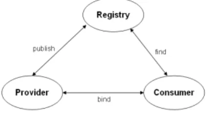
The Web service architecture is defined by 3WC in order to determinate a com-mon set of concepts and relationships that allow different implementations work-ing together [4]. Figure 1 shows a graphical representation of the traditional Web service architecture. The conventional Web service architecture consists of three entities, the service provider, the service registry and the service consumer. The service provider creates or simply offers the Web service. The service provider needs to describe the Web service in a standard format, which is often XML, and publish it in a central service registry. The service registry contains additional information about the service provider, such as address and contact of the pro-viding company, and technical details about the service. The service consumer retrieves the information from the registry and uses the service description ob-tained to bind to and invoke the Web service. The appropriate methods are depicted in Figure 1 by the keywords “publish”, “bind” and “find”.
Fig. 1. Conventional architecture of Web services
Web services architecture is loosely coupled, service oriented. The Web Ser-vice Description Language (WSDL) uses the XML format to describe the meth-ods provided by a Web service, including input and output parameters, data types and the transport protocol, which is typically HTTP, to be used. The Uni-versal Description Discovery and Integration standard (UDDI) suggests means to publish details about a service provider, the services that are stored and the opportunity for service consumers to find service providers and Web service de-tails. The Simple Object Access Protocol (SOAP) is generally used for XML formatted information exchange among the entities involved in the Web service model.
4.2 Proposed Web service architecture
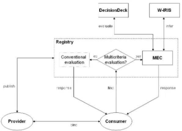
The proposed framework extends the conventional Web services architecture by adding, in the registry, a new Multicriteria Evaluation Component (MEC) devoted to multicriteria evaluation. The general schema of the extended archi-tecture is given in Figure 2. According to the requirement of the consumer, the registry opts either for conventional evaluation or for multicriteria evaluation.
By default, the registry uses conventional evaluation; multicriteria evaluation is used only if the consumer explicitly specifies this in the SOAP message addressed to the registry. This ensures the flexibility of the proposed architecture.
The application of a multicriteria method needs the definition of a set of preference parameters. The definition of these parameters needs an important cognitive effort from the consumer. To reduce this effort, MEC uses specific Web service called W-IRIS which is a Web version of IRIS (Interactive Robustness analysis and Parameters Inference for multicriteria Sorting Problems) [5] system permitting to infer the different preference parameters.
Fig. 2. Extended architecture of Web services
As we can see in Figure 2, the three basic operations denoted by “publish”, “bind” and “find” still exist. Two additional operations, denoted by keywords “infer” and “evaluate” are included in the extended architecture. The first per-mits to handle data exchange between MEC and W-IRIS. The latter perper-mits to handle data exchange between MEC and DecisionDeck platform, presented in the end of this subsection.
To achieve the interaction among the entities of the extended Web service model, we need to extend some SOAP protocoles and add new ones. More specif-ically, we need to extend protocols of consumer request to registry and registry response to consumer; and add the ones relative to MEC request to W-IRIS and W-IRIS response to MEC. A detailed description of the proposed architecture is given in Figure 3.
Fig. 3. Dynamics of the system
One important remark to evoke at this level is relative to the fact that sev-eral providers may be implied by the consumer or by the registry and that a given provider may invoke other providers. This is illustrated by the discounted arrows between provider-1 and provider-N in Figure 3. It is important to men-tion that the proposed architecture still applies since the multicriteria evaluamen-tion implies only the providers directly invoked by the consumer or the registry. In addition, we suppose that the evaluations of the services proposed by directly invoked providers include the evaluations of the ones indirectly invoked by these providers.
As we will be explained latter, W-IRIS permits to infer the different prefer-ence parameters needed to apply multicriteria evaluation using ELECTRE TRI method. The inference procedure included in W-IRIS needs the resolution of different mathematical programs. For this purpose, W-IRIS includes the solver GLPK, which is an open-source and free package (see [11]).
The current version of MEC supports the advanced multicriteria method ELECTRE TRI (see [6]) and several elementary methods (weighted sum, con-junctive and discon-junctive rules and the majority rule). Additional methods will be included in the future via the DecisionDeck platform. The DecisionDeck plat-form, which is under development, is issued from D2-Decision Deck project that has started in 2003 under the name EVAL, an acronym which refers to an ongoing research project funded by the Government of the Walloon region (Belgium). The aim is to develop a Web-based platform to assist decision mak-ers in evaluating alternatives in a multicriteria and multi-experts context. The EVAL platform is currently available on the collaborative development Web site www.sourceforge.org.
In the rest of this section, we detail the required extension/addition to sup-port data exchange between the different entities of the proposed architecture.
4.3 Consumer—Registry communication
The XML schema of consumer request to registry is given in Figure 4. The con-sumer may choose between two types of evaluations: mono-criterion or multicri-teria. This ensured by the <choice> tag in Figure 4. The monocriterion−evaluation
element in this figure refers to conventional evaluation. It will not be detailed here. The multicriteria−evaluation element corresponds to multicriteria
evalua-tion. It is a complex type composed of four elements: result−type, evaluation−criteria,
sorting−data, and parameters.
Type of result (<result−type> tag) The consumer may indicate the type of result
of multicriteria evaluation, which may be “choice”, “ranging” or “sorting” (see Section 5.6). The default value is “choice” indicating that a restricted subset of compositions will be returned to the consumer.
Evaluation criteria (<evaluation−criteria> tag) The consumer must indicate at
least two QoS evaluation criteria to be used to evaluate and compare the different potential compositions. For each criterion, it specifies (i) the name, which may
be any one from the list given in Table 1; and (ii) zero or several preference parameters. For each preference parameter, it indicates the name and the value. The name is one of the following list:
– Weight – Indifference threshold – Preference threshold – Veto threshold – Aspiration level – Reservation level <xsd:schema xmlns:xsd="http://www.w3.org/2000/10/XMLSchema"> <xsd:complexType element name="find_service">
<xsd:choice>
<xsd:element name="monocriterion_evaluation" type="monoType"> <xsd:element name="multicriteria_evaluation" type="mecType"> </xsd:choice> </xsd:complexType <xsd:complexType name="monoType"> ... </xsd:complexType> <xsd:complexType name="mecType"> <xsd:sequence>
<xsd:element name="result_type" type="token" #REQUIRED> <xsd:element name="evaluation_criteria"> <xsd:element name="sorting_data"> <xsd:element name="parameters"> </xsd:sequence> </xsd:complexType> <xsd:complexType name="evaluation_criteria"> <xsd:sequence> <xsd:group ref="criteriaGroup"> </xsd:sequence> </xsd:complexType> <xsd:group name="criteriaGroup"> <xsd:sequence>
<xsd:element name="criterion" type="criterionType" minOccurs="2"> </xsd:sequence>
</xsd:group>
<xsd:complexType name="criterionType"> <xsd:sequence>
<xsd:element name="criterion_name" type="token" #REQUIRED> <xsd:element name="preference_parameters"> </xsd:sequence> </xsd:complexType> <xsd:complexType name="preference_parameters"> <xsd:sequence> <xsd:group ref="preferenceGroup"> <xsd:sequence> </xsd:complexType> <xsd:group name="preferenceGroup"> <xsd:sequence>
<xsd:element name="preference_parameter" type="preference_parameterType" minOccurs="0"> <xsd:sequence>
</xsd:group>
<xsd:complexType name="preference_parameterType"> <xsd:sequence>
<xsd:element name="name" type="token" #REQUIRED> <xsd:element name="value" type="anyType" #REQUIRED> </xsd:sequence>
</xsd:complexType>
<xsd:complexType name="sorting_data">
<xsd:element name="categories_number" type="xsd:positiveInteger"> <xsd:element name="profiles"> <xsd:element name="assignment_examples"> </xsd:complexType> <xsd:complexType name="profiles"> <xsd:sequence> <xsd:group ref="profilesGroup"> </xsd:sequence> </xsd:complexType> <xsd:group name="profilesGroup"> <xsd:sequence>
<xsd:element name="profile" type="profileType" minOccurs="0"> </xsd:sequence>
</xsd:group>
<xsd:complexType name="profileType"> <xsd:sequence>
<xsd:element name="name" type="xsd:String" #REQUIRED>
<xsd:group name="criteriaGroup" type="criteriaGroupType" minOccurs="xsd:positiveInteger"> </xsd:sequence>
</xsd:complexType>
<xsd:complexType name="criterionType"> <xsd:sequence>
<xsd:element name="name" type="token" #REQUIRED> <xsd:element name="value" type="anyType" #REQUIRED>> </xsd:sequence> </xsd:complexType> <xsd:complexType name="assignment_examples"> <xsd:sequence> <xsd:group ref="assignment_exampleGroup"> </xsd:sequence> </xsd:complexType> <xsd:group name="assignment_exampleGroup"> <xsd:sequence>
<xsd:element name="assignment_example" type="assignment_exampleType" minOccurs="0"> </xsd:sequence>
</xsd:group>
<xsd:complexType name="assignment_exampleType"> <xsd:sequence>
<xsd:element name="compositionID" type="compositionType"> <xsd:element name="cMin" type="xsd:positiveInteger"> <xsd:element name="cMax" type="xsd:positiveInteger"> </xsd:sequence>
</xsd:complexType>
<xsd:group name="parameters"> <xsd:sequence>
<xsd:element name="parameter_name" type="token" #REQUIRED> <xsd:element name="value" type="anyType" #REQUIRED> </xsd:sequence>
</xsd:group>
Fig. 4. XML schema of consumer request to registry
The weights represent the relative importance of the different QoS evaluation criterion according to the aspiration of the consumer. The next three parameters are often used within outranking relation-based multicriteria methods (see [6]).
The indifference and preference thresholds are used to model the imprecision and uncertainty in the consumer preferences. The veto threshold is often used to compute the discordance index as will be explained latter. The aspiration
level is the minimal (maximal, resp.) value defined on an evaluation criterion
and which should be exceeded (resp. not exceeded) by each composition to be acceptable. One or several aspiration levels may be defined for different criteria. The reservation level represents the minimal value on a given criterion that should be verified by any potential composition. The reservation level needs to be defined for all the evaluation criteria.
Sorting data (<sorting−data> tag) It applies when the type of result is
“sort-ing”, i.e., a classification of different composite Web services into a set of pre-defined categories (see Section 5.6). These categories are pre-defined in terms of a set of profile limits representing the boundaries between these categories. The consumer should provide: (i) the number of categories; (ii) the profile limits; and (iii) a set of assignment examples. The number of categories is optional. The default value for the number of categories is 3. The profile limits may be either provided by the consumer or generated automatically, as explained in Section 4.4. This second option is included to reduce the cognitive effort of the consumer. A profile limit is defined as a vector of m elements, where m is the number of evaluation criteria. An advanced definition of a profile may need the use of indifference threshold, preference threshold and/or veto threshold.
The consumer should also provide a set of assignment examples which will be used to infer the preference parameters. More details on how these assignment examples are defined and used will be given in Section 4.4.
Parameters (<parameters> tag) This optional element is used to cope with some
multicriteria methods that require the definition of some technical parameters. For instance the cutting level is used with some multicriteria outranking methods to validate or invalidate the outranking relation. Note that this parameter should belongs to [0.5, 1] and when omitted, the value 0.5 is used.
The XML schema of registry response to consumer is given in Figure 5. The registry indicates the list of recommended compositions. As it is shown in Figure 5, three types of recommendations are possible: choice, ranging or classification. This is ensured by the <choice> tag in Figure 5. A brief description of these different types of recommendation follows.
– List of best compositions. This applies when the type of result is “choice”. In this case, the recommendation of MEC is a restricted set of equivalent compositions from which the user should choose one for application. – A ranging of compositions. This applies when the type of result is “ranging”.
The recommendation of MEC in this case is a list of compositions ordered from the best to the worst. These information are handled by the <order> element in Figure 5.
– A classification of compositions. This last case applies when the type of result is “sorting”. The output of MEC is a list of compositions, each one
is characterized by its category indicated by the <category> element in Figure 5.
<xsd:schema xmlns:xsd="http://www.w3.org/2000/10/XMLSchema"> <xsd:complexType element name="serviceList">
<xsd:sequence> <xsd:choice> <xsd:element name="choice"> <xsd:element name="ranging"> <xsd:element name="classification"> </xsd:choice> </xsd:sequence> </xsd:complexType> <xsd:complexType name"choice"> <xsd:sequence> <xsd:group ref="choiceGroup"> </xsd:sequence> </xsd:complexType> <xsd:group name="choiceGroup" <xsd:sequence>
<xsd:element name="serviceInfos" type="choiceInfos" minOccurs="1"> </xsd:sequence>
</xsd:group>
<xsd:complexType name="choiceInfos">
<xsd:element name="compositionID" type="compositionType"> </xsd:complexType> <xsd:complexType name"ranging"> <xsd:sequence> <xsd:group ref="rangingGroup"> </xsd:sequence> </xsd:complexType> <xsd:group name="rangingGroup" <xsd:sequence>
<xsd:element name="serviceInfos" type="rangingInfos" minOccurs="1" maxOccurs="xsd:positiveInteger"> </xsd:sequence>
</xsd:group>
<xsd:complexType name="rangingInfos">
<xsd:element name="compositionID" type="compositionType"> <xsd:element name="order" type="xsd:positiveInteger"> </xsd:complexType> <xsd:complexType name"sorting"> <xsd:sequence> <xsd:group ref="sortingGroup"> </xsd:sequence> </xsd:complexType> <xsd:group name="sortingGroup" <xsd:sequence>
<xsd:element name="serviceInfos" type="sortingInfos" minOccurs="1" maxOccurs="xsd:positiveInteger"> </xsd:sequence>
</xsd:group>
<xsd:complexType name="sortingInfos">
<xsd:element name="compositionID" type="compositionType"> <xsd:element name="category" type="xsd:string">
<xsd:complexType>
4.4 MEC—W-IRIS communication
The W-IRIS is a special kind of Web service used by MEC to infer the preference parameters to use with ELECTRE TRI method. An brief overview of ELECTRE TRI is provided in Appendix A. This method is used by MEC to assign compos-ite Web services into different categories. It applies when “type of result” in the SOAP message sent by the consumer to registry is “sorting” (see Figure 4). The XML schema of the “infer” SOAP message sent by the MEC to W-IRIS is given in Figure 6. It contains the same information included in the “sorting−data”
ele-ment given in Figure 4. To avoid redundancy, the “sorting−data” is not detailed
in Figure 6.
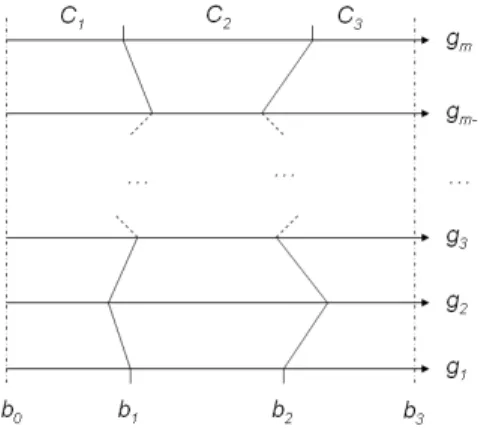
In the most general case, the inputs of W-IRIS are: (i) the number of cat-egories, (ii) a set of profile limits, and (iii) a set of assignment examples. All of these data are extracted from the SOAP message sent by the consumer to registry detailed in the previous subsection (see Figure 4). As underlined ear-lier, the number of categories is an optional parameter and when it is omitted, three categories are automatically used. These categories are denoted C1, C2,
and C3. Category C3 corresponds to recommended compositions and category
C1 corresponds to unrecommended compositions. Category C2 corresponds to
intermediate compositions. As introduced above, the categories are defined in terms of a set of profile limits. Figure 7 shows the definition of categories C1,
C2, and C3 in terms of two profile limits b1 and b2. Each profile is defined as
a vector of m elements where m is the number of considered QoS evaluation criteria, denoted g1, g2, · · · , gm in Figure 7. Profiles b0 and b4 are defined as a
vector of lower and higher boundaries of evaluation criteria scales.
In the case where the profile limits are not provided by the consumer, they will be automatically constructed by MEC. To this purpose, the measurement scale of each QoS evaluation criterion included in the “find” SOAP message sent by the consumer to the registry is subdivided into three equal intervals. Then, profile limits are defined by joining the limits of these intervals on the different evaluation criteria.
<xsd:schema xmlns:xsd="http://www.w3.org/2000/10/XMLSchema"> <xsd:complexType element name="infer">
<xsd:sequence>
<xsd:element name="sorting_data"> </xsd:sequence>
</xsd:complexType>
<xsd:complexType name="sorting_data">
<xsd:element name="categories_number" type="xsd:positiveInteger"> <xsd:element name="profiles">
<xsd:element name="assignment_examples"> </xsd:complexType>
....
The set of assignment examples are defined as follows. First, MEC generates a set of fictive compositions. Each fictive composition kf is associated with a
vector of m elements:
(g1(kf), g2(kf), · · · , gm(kf)),
where m is the number of QoS evaluation criteria. Evaluations gj(kf) (j =
1, · · · , m) are defined such that kf may be assigned to two succussive categories.
For better explanation, consider two categories Ciand Cj and let bhbe the
pro-file limit between Ci and Cj with evaluation vector (g1(bh), g2(bh), · · · , gm(bh)).
Then, a fictive composition kf is defined such that its performances on a subset
of QoS evaluation permits to assign it to Ci and the rest permits to assign it to
Cj.
Fig. 7. Definition of classes C1, C2and C3 in terms of the profile limits
XML schema of W-IRIS “inference−ouptut” SOAP message to MEC is given
in Figures 8. It is a collection of preference parameters and the corresponding values. These parameters will be used by MEC to apply ELECTRE TRI.
5
Multicriteria evaluation component
The general schema of multicriteria evaluation component (MEC) is depicted in Figure 2. Basically, it takes as input a set of composite Web services and a set of QoS evaluation criteria and generates a set of recommended composi-tions. The final choice should be performed by the consumer, based on the MEC recommendation.
In the rest of the paper, K = {k1, k2, · · · , kn} denotes a set of n
poten-tial composite Web services and I = {1, 2, · · · , n} denotes the indices of these services. The solution proposed to construct set K will be detailed in Section 7.
<xsd:schema xmlns:xsd="http://www.w3.org/2000/10/XMLSchema"> <xsd:complexType element name="inference_output">
<xsd:sequence> <xsd:group ref="preference_parametersGroup"> </xsd:sequence> </xsd:complexType> <xsd:group name="preference_parametersGroup"> <xsd:sequence>
<xsd:element name="preference_parameter" type="preference_parameterType" minOccurs="1"> <xsd:sequence>
</xsd:group>
<xsd:complexType name="preference_parameterType"> <xsd:sequence>
<xsd:element name="name" type="token" #REQUIRED> <xsd:element name="value" type="anyType" #REQUIRED> </xsd:sequence>
</xsd:complexType>
Fig. 8. XML schema of W-IRIS response to MEC
5.1 Definition of QoS evaluation criteria
The set of QoS evaluation criteria to be used is extracted from the “find” SOAP message sent by the consumer to the registry (see Section 4.3). At least two QoS evaluation criteria should be provided. The set of evaluation criteria will be denote by F = {g1, g2, · · · , gm} in the rest of the paper. Theoretically, there is
no limit to the number of criteria. We observe, however, that a large set increases the cognitive effort required from the consumer and a few ones do not permit to encompass all the facets of the selection problem.
5.2 Quantification of evaluation criteria
Quantification permits to transform qualitative evaluation criteria into quantita-tive ones by assigning values to the qualitaquantita-tive data. This is useful for mostly of multicriteria methods based on weighted-sum like aggregation decision rules. The most used quantification method is the scaling one. The quantification process consists in the definition of a measurement scale as the one mentioned earlier and then to associate to each level of the scale a numerical value. For example, the numbers 1, 2, 3, 4 and 5 may be associated to the fifth levels scale introduced in Section 3, going from very low to very high. Note, however, that the set of mathematical operations authorized is the same as the one mentioned in Section 3, i.e., “equal to” (=), “less than” (<), “more than” (>).
5.3 Generation of performance table
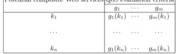
Once potential composite Web services are constructed and evaluation criteria are identified, the next step consists in the evaluation of all these composite Web services against all the evaluation criteria in F . The evaluation of a composite Web Service ki ∈ K in respect to criterion gj∈ F is denoted gj(ki). The matrix
of the performance table is given in Figure 9. The computing of gj(ki), ∀i ∈ I,
∀j ∈ F , will be dealt with in Section 8.
Potential composite Web services QoS evaluation criteria
g1 · · · gm k1 g1(k1) · · · gm(k1)
· · · · · · · · · · · ·
kn g1(kn) · · · gm(kn)
Fig. 9. General structure of performance table
5.4 Definition of preference parameters
Most of multicriteria methods require the definition of a set of preference pa-rameters. Two cases hold here: either the preference parameters are provided explicitly by the consumer and extracted from the “find” SOAP message to the registry; or inferred by W-IRIS based on the assignment examples equally extracted from the “find” SOAP message sent by the consumer.
5.5 Multicriteria evaluation
The input for this step are the performance table and the preference parameters. The objective of multicriteria evaluation is to evaluate and compare the different compositions in K.
As signaled above the advanced multicriteria method ELECTRE TRI and four elementary methods (weighted sum, conjunctive and disjunctive rules, and the majority rule) are incorporated in the framework. Additional methods will be included in the future. The application of ELECTRE TRI is reported in Section 9.
5.6 Recommendation
As underlined above, three types of recommendations are possible within the proposed framework. Based on the specifications of the consumer, one of the following results is provided to it:
– one or a restricted set of composite Web services;
– a ranging of composite Web services from best to worst with eventually equal positions;
– a classification of composite Web services into different pre-defined cate-gories.
These three types of result correspond in fact to the three ways usually used to formalize multicriteria problems as identified by [19]: choice, ranking and
6
W-IRIS Web service
W-IRIS implements a Web version of IRIS (Interactive Robustness analysis and Parameters Inference for multicriteria Sorting Problems) system. IRIS supports a methodology of inference initially proposed in [18] (see also [17]). Here, we will shortly introduce the principle of the inference procedure included in W-IRIS.
The input for the inference procedure is the set of assignment examples pro-vided by the consumer. Let K∗ be the set of these assignment examples. We
define two sets S+ = {(k, b
h) ∈ K∗× B: that the consumer states that kSbh}
and S−= {(k, b
h) ∈ K∗× B: that the consumer states that ¬(kSbh)}. Relation
S is the outranking binary relation (see Appendix A) defined such that kSbh
means that the evaluation of composition k upon all evaluation criteria is at least as good as the evaluation of the profile bh (lower limit of category Ch+1). The
idea of the inference procedure consists in searching a set of preference parame-ters that permit to re-do the assignment examples provided by the consumer. This can be obtained by resolving the following system:
σ(k, bh) ≥ λ, ∀(k, bh) ∈ S+ σ(k, bh) < λ, ∀(k, bh) ∈ S− λ ∈ [0.5, 1] qj(bh) ≤ pj(bh) ≤ vj(bh), ∀(j, h) ∈ F × B Pm j=1wj = 1; wj ≥ 0, ∀j ∈ F where:
– σ(k, bh) ∈ [0, 1] is the credibility degree that measures the extent to which
composition k outranks profile limit bh;
– λ is the cutting level used to validate or invalidate the outranking relation; – qj(bh), pj(bh) and vj(bh) (j = 1, · · · , m) are the indifference, preference and
veto threshold associated with profile limit bh; and
– wj (j = 1, · · · , m) is the weights of evaluation criteria.
Some of these concepts are introduced in Section 4.3. Further details are given in Appendix A, along with the presentation of ELECTRE TRI method. This system can be expressed through a mathematical program having as variables the parameters to infer. Then, the values for these parameters are obtained by maximizing the minium slack for this system of constraints. The inferred parameters are then used to apply ELECTRE TRI.
To construct the system, W-IRIS uses the data extracted from the XML document corresponding to the “evaluate” request sent by MEC to W-IRIS. Then W-IRIS uses the routines of GLPK1 to resolve the mathematical program
issued from the system above.
1 More information on GLPK solver and routines is available at
7
Constructing potential composite Web services
Following Menasc´e [14], a Web service is defined as follows. Definition 1 A Web service Si is a tuple (Fi, Qi, Hi), where:
– Fi is a description of the service’s functionality,
– Qi is a specification of its QoS evaluation criteria, and
– Hi is its cost specification.
Menasc´e [14] uses the term “attribute” instead of “criteria”. The last one is more general and hence is adopted here. A Web service’s QoS evaluation criterion may be any one of the list provided in Table 1. A Web service’s cost is often related to its quality. Faster, reliable, secure services will be more expensive, for example, but there could also be penalties associated with not meeting certain QoS goals or service-level agreements (SLAs) [14].
A composition operation implies several individual Web services. The rela-tionships among the individual Web services may be represented by a connected and directed graph G = (X, V ) where X = {Si, Sj, · · · , Sm} is the set of
in-dividual Web services and V = {(Si, Sj) : Si, Sj ∈ X ∧ Si can invoke Sj}.
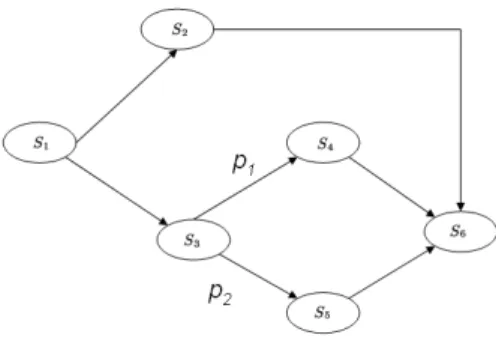
G = (X, V ) is called the composition graph. Figure 10, which is reproduced
from [14], presents a composition graph example implying six individual Web services S1, S2, S3, S4, S5 and S6.
Fig. 10. An example of composition graph
The arcs in this figure represent different types of invocation. These last ones correspond to different BPEL constructors. The basic BPEL constructors are:
• Sequential invocation. A Web service is activated as a result of the completion
of one of a set of mutually exclusive predecessor activities. These activities may be listed with the XML <sequence> tag, that is, in lexical order.
• Parallel invocation (fork). It represents a point in the process where a single
thread of control splits into multiple threads of control which can be executed in parallel. This pattern is supported by BPEL using XML <flow> tag.
Example: S1 in Figure 10 which can invoke S2 and S3in parallel.
• Probabilistic invocation. A probability value p on an outgoing arrow from Si
to Sj indicates that Siinvokes Sj with probability p. If no value is indicated,
the probability is assumed to be 1. Example: S3in Figure 10 which can invoke
S4with probability p1 or S5with probability p2.
• Conditional invocation. Represents a situation where one or several branches
are chosen. The first situation can directly be implemented using <switch> constructor and the second through control links inherited from XLANG. There is no example of conditional invocation in Figure 10.
• Synchronized invocation (join). A Web service is activated only when all
of its predecessor Web services have completed. It can be implemented us-ing control links inherited from XLANG. Example: S6 in Figure 10 which
requires the completion of Web services S4and S5.
We assume that each Web service Si has a unique functionality Fi. In turn,
the same functionality may be provided by different providers. Let Pi be the
collection of providers supporting functionality Fi of Web service Si: Pi =
{s1
i, s2i, · · · , snii} where ni is the number of providers in Pi. A composite Web
service is defined as follows.
Definition 2 Let S1, S2, · · · , Sn be a set of n individual Web services such that
Si= (Fi, Qi, Hi) (i = 1, · · · , n). Let Pi be the collection of Web services
support-ing functionality Fi. Let G = (X, V ) be the composition graph associated with
S1, S2, · · · , Sn. A composite Web service k is an instance {s1, s2, · · · , sn} of
G defined such that s1∈ P1, s2∈ P2, · · · , sn ∈ Pn.
It is clear that this definition may lead to a large number of compositions. Some solutions to avoid this problem will be introduced in Section 10.
To take into account the invocation probabilities associated with some Web services, we define a new function, called π, as follows:
π: X × X → [0, 1]
Si× Sj→ π(Si, Sj)
The number π(Si, Sj) represents the probability that Si invokes Sj.
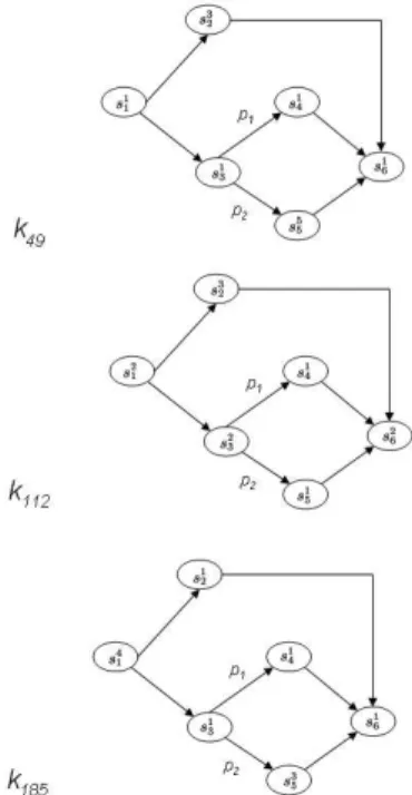
Example 1. Consider the graph of Figure 10 and suppose that:
– P1= {s11, s21, s31, s41} – P2= {s12, s22, s32} – P3= {s13, s23} – P4= {s14} – P5= {s15, s25, s35, s45, s55} – P6= {s16, s26}
where sji is the jth provider of Web service Si. Then, the following are some
composite Web services:
– k49 associated with G49= (X49, V49) where:
• X49= {s11, s32, s31, s14, s55, s16}
• V49= {(s11, s32); (s11, s13); (s32, s16); (s31, s14); (s13, s55); (s14, s16); (s55, s16)}
• π(s1
3, s14) = p1; π(s13, s55) = p2
– k112 associated with G112= (X112, V112) where:
• X112= {s21, s32, s32, s14, s15, s26}
• V112= {(s21, s32), (s21, s23), (s23, s41), (s23, s15); (s14, s26); (s15, s26)}
• π(s2
3, s14) = p1; π(s23, s15) = p2
– k185 associated with G185= (X185, V185) where:
• X185= {s41, s12, s31, s14, s35, s16}
• V185= {(s41, s12); (s41, s13); (s13, s41); (s13, s35); (s14, s16); (s35, s16)}
• π(s1
3, s14) = p1; π(s13, s35) = p2
Figure 11 shows graphically the composite Web services k49, k112 and k185.
Fig. 11. Composed Web services k49, k112 and k185
To construct the set of potential compositions, we have incorporated two algorithms in the MEC. The first one, called CompositionGraph and given below,
permits the construction of the composition graph. In this algorithm, Γ+(x)
returns the set of successors of node x: Γ+(x) = {y ∈ X : (x, y) ∈ V }. The input
of CompositionGraph algorithm is the description of the different individual Web services stored in the UDDI registry and the invocation probability function π. The output is the composition graph G defined earlier. The algorithm runs in
O(n2) where n is the number of Web services.
Algorithm CompositionGraph
INPUT: S = S1, S2, · · · , Sm: the set of Web services
OUTPUT: G = (X, V ): composition graph
X ← S Z ← S curr−node← S1 WHILE Z 6= ∅ FOR each Sj∈ X IF Sj∈ Γ+(curr−node)
THEN V ←(curr−node,Sj)
END−FOR
Z ← Z \ curr−node
curr−node← pick a node in Z
END−WHILE
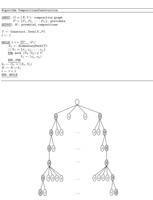
The second algorithm, given hereafter, is CompositionsConstruction that generates the potential compostions. The algorithm CompositionsConstruction proceeds as follows. First a tree T is constructed using Construct−Tree. The
inputs for this procedure is the set of nodes X and the set of providers for each node in X: P = {P1, P2, · · · , Pn}. The tree T is constructed as follows. The nodes
of the ith level are the providers in Pi. For each node in level i, we associate
the providers in set Pi+1 as sons. The same reasoning is used for i = 1 to n − 1.
The nodes of the n − 1th level is associated with the providers in Pn. Finally, a
root r is added to T as the parent of nodes in the first level (representing the providers in P1). Then, the set of nodes for each composition is obtained as an
elementary path in T . Figure 12 shows a schematic representation of the tree as-sociated with composition graph given in Figure 10. The first elementary path is composed of s1
1, s12, s13, s14, s15 and s61. The last elementary path is s41, s32, s23, s14, s55
and s2
6. Thus, the node set of k1 is X1= {s11, s12, s13, s14, s15, s16} and the node set
Algorithm CompositionsConstruction INPUT: G = (X, V ): composition graph
P = {P1, P2, · · · , Pn}: providers
OUTPUT: K: potential compositions
T ← Construct−Tree(X,P ) t ← 1 WHILE t <=Qn i=1|Pi| Xt← ElementaryPath(T ) //Xt= {s·1, s·2, · · · , s·n} FOR each (Sh, Sk) ∈ V Vt← (s·h, s·k) END−FOR kt← Gt= (Xt, Vt) K ← K ∪ kt t ← t + 1 END−WHILE r . . . . . . . . . . . . s1 1 s 2 1 s 3 1 s 4 1 s1 2 s 2 2 s 3 2 s3 2 s2 2 s1 2 s31 s 2 3 s 1 3 s2 3 s1 4 s41 s1 5 s 2 5 s 3 5 s 4 5 s5 5 s51 s 2 5 s 3 5 s 4 5 s5 5 s16 s 2 6 s 1 6 s 2 6 . . .
Fig. 12. Schematic representation of tree T
Once the collections of providers of the different compositions are defined, al-gorithm CompositionsConstruction use the composition graph G to construct the different compositions as instances of graph G.
The complexity of algorithm CompositionsConstruction is O(r1× (r2+
r3)) where r1 = |V | is the cardinality of V , r2 =
Qn
i=1|Pi| is the number of
8
Evaluation of compositions
As defined earlier, a potential composition is an instance of the composition graph G = (X, V ). Each composition can be seen as collection of individual Web services. The evaluation provided by the UDDI registry are relative to these individual Web services. However, to evaluate and compare the different potential compositions, it is required to define a set of rules to combine the partial evaluations (i.e. in respect to individual Web services) to obtain partial evaluations that apply to the whole composition.
To compute the partial evaluations gj(ki) (j = 1, · · · , m) of the different
compositions ki(i = 1, · · · , n), we need to define a set of m aggregation operators
Φ1, Φ2, · · · , Φm, one for each evaluation criterion. The partial evaluation of a
composition ki on criterion gj, gj(ki), is computed as follows. It consists in
applying a bottom-top scan on graph Gi= (Xi, Vi) and to apply the aggregation
operator Φjon each node. Algorithm PartialEvaluation below implements this
idea. It runs on O(r2) where r = |X| is the number of nodes in the composition
graph.
The valuation, in respect to criterion gj, of a node x ∈ Xi, denoted vj(x), is
computed as follows:
vj(x) = Φj[gj(x), Ω(Γ+(x))]
Recall that Γ+(x) is the set of successors of node x. The operator Ω involves
nodes on the same level and may be any aggregation operator such as sum, product, max, min, average, etc. The operator Φj implies nodes on different
levels and vary according to the BPEL constructors (see Section 7) associated with node x. It may be the sum, product, max, min, or average.
Algorithm PartialEvaluation INPUT: ki= Gi(Xi, Vi): composition
Φj: aggregation operators
OUTPUT: gj(ki): partial evaluation of ki on gj
Lr← {s ∈ Xi: Γ+(s) = ∅} Z ← ∅ WHILE Z 6= Xi FOR each x ∈ Lr vj(x) ← Φj[gj(x), Ω(Γ+(x))] Z ← ZS{x} END−FOR Lr← {s ∈ Xi : vj(w) is computed ∀w ∈ Γ+(s)} END−WHILE
gj(ki) ← vj(s) where s is the root of Gi
It is important to note that when the criterion is ordinal, it is not possible to use the probability associated with the branches of a <switch> constructor. To avoid this problem, we may use one of the following rules (other rules may also apply):
– ignore the probabilities and proceed as with the <flow> BPEL constructor; – use the partial evaluation associated with the most probable branch; – use the majority rule (when there are at least three branches);
– use the intermediate level between the partial evaluations associated with most probable branch and least probable branch;
– use the intermediate level between the highest partial evaluation and the lowest partial evaluation.
In the following, we provide the proposed formula for computing vj(x) (j =
1, · · · , 4) for response time, availability, cost and security evaluation criteria, denoted g1, g2, g3 and g4, respectively. Evaluation criteria g1 and g3 are to be
minimized while criteria g2 and g4 are to be maximized. The three first criteria
are cardinal. The latter is an ordinal one.
First, we mention that the following formula apply for non-leaf nodes, i.e.,
x ∈ Xi such that Γ+(x) 6= ∅. For leaf nodes, i.e. x ∈ Xi such that Γ+(x) = ∅,
the partial evaluation on a criterion gj is simply vj(x) = gj(x).
Response time (g1) The response time of a non-leaf node x is computed as
follows: v1(x) = g1(x) + max{v1(y) : y ∈ Γ+(x)} (1) or v1(x) = g1(x) + X y∈Γ+(x) π(x, y) · v1(y) (2)
Equation (1) applies for the <flow> or the sequential BPEL constructors. Equation (2) applies when the constructor <switch> is used. Here: Φ1 is the
sum and Ω is the max (for Equation (1)) or the sum (for Equation (2)).
Availability (g2) For the availability, two formulae may be applied:
v2(x) = g2(x) · Y y∈Γ+(x) v2(y) (3) or v2(x) = g2(x) · X y∈Γ+(x) π(x, y) · v2(y) (4)
Equation (3) applies for the <flow> BPEL or the sequential constructors. Equation (4) applies when the constructor <switch> is used. Here: Φ2 is the
Cost (g3) For cost criterion, two formula may be used: v3(x) = g3(x) + X y∈Γ+(x) v3(y) (5) or v3(x) = g3(x) + X y∈Γ+(x) π(x, y) · v3(y) (6)
Equation (5) applies for the <flow> or the sequential BPEL constructors. Equation (6) applies when the constructor <switch> is used. Here, the sum operator is used for both Φ3and Ω.
Security (g4) Finally, for security criterion, we have:
v4(x) = min{g4(x), min
y∈Γ+(x){v4(y)}} (7)
Here, both Φ4and Ω are the min operator. Recall that security criterion is an
ordinal one. Equation (7) applies when the <flow> BPEL constructor is used. When the constructor <switch> is used, one of the rules mentioned above is used.
These different equations are illustrated through Example 2 that follows.
Example 2. For better illustration of the previous formula, consider again the
composition graph of Figure 10 and the three compositions k49, k112 and k185
given in Figure 11. Suppose that p1= 0.4 and p2= 0.6. The objective is to show
the computing of partial evaluations of k49, k112 and k185 in respect to four
evaluation criteria: Response time (g1), Availability (g2), Cost (g3) and Security
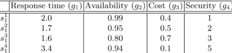
(g4). The evaluation of the providers of Web services S1to S6in respect to g1, g2,
g3 and g4are given in Tables 2 to 7, respectively. Recall that evaluation criteria
g1 and g3 are to be minimized while criteria g2 and g4 are to be maximized.
Recall also that the three first criteria are cardinal. The latter is ordinal for which the following five-levels scale is used: 1:“very low”, 2: “low”, 3: “average”, 4: “high”, and 5: “very high”.
Response time (g1) Availability (g2) Cost (g3) Security (g4)
s1 1 2.0 0.99 0.4 1 s2 1 1.7 0.95 0.5 2 s3 1 1.6 0.80 0.7 3 s4 1 3.4 0.94 0.1 5
Table 2. Evaluations of providers of Web service S1
Illustrating now the computing for partial evaluation of composition k49in
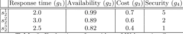
Response time (g1) Availability (g2) Cost (g3) Security (g4) s1 2 2.0 0.99 0.7 5 s2 2 3.0 0.89 0.6 2 s3 2 2.5 0.82 0.4 1
Table 3. Evaluations of providers of Web service S2
Response time (g1) Availability (g2) Cost (g3) Security (g4)
s1
3 2.0 0.85 0.4 4
s2
3 1.7 0.84 0.5 2
Table 4. Evaluations of providers of Web service S3
Response time (g1) Availability (g2) Cost (g3) Security (g4)
s1
4 1.8 0.89 0.3 5
Table 5. Evaluations of providers of Web service S4
Response time (g1) Availability (g2) Cost (g3) Security (g4)
s1 5 3 0.86 0.5 1 s2 5 1.5 0.60 0.6 2 s3 5 2 0.99 0.8 5 s4 5 2.5 0.82 1.2 4 s5 5 3 0.90 0.6 3
Table 6. Evaluations of providers of Web service S5
Response time (g1) Availability (g2) Cost (g3) Security (g4)
s1
6 3 0.8 0.23 5
s2
6 2.5 0.92 0.5 3
Table 7. Evaluations of providers of Web service S6
is used on G49 = (X49, V49). Details of computing are given below. Recall that
aggregation mechanism Φ1associated with g1is the sum operator.
First, for leaf-node s1
6, we have v1(s16) = g1(s16) = 3.0. Then, for nodes s14and
s5 5, we apply Equation (1): v1(s14) = g1(s14) + max{v1(s16)} = 1.8 + 3.0 = 4.8. v1(s55) = g1(s55) + max{v1(s16)} = 3.0 + 3.0 = 6.0.
For node s1 3, we apply Equation (2): v1(s13) = g1(s13) + (p1· v1(s14) + p2· v1(s55)) = 2.0 + (0.4 × 4.8 + 0.6 × 6) = 7.52. For node s3 2, we apply Equation (1): v1(s32) = g1(s32) + max{v1(s16)} = 2.5 + 3.0 = 5.5. For node s1 1, we apply Equation (1): v1(s11) = g1(s11) + max{v1(s32), v1(s13)} = 2.0 + max{5.5, 7.52} = 2.0 + 7.52 = 9.52.
The partial evaluation of composition k49 on criterion response time is then
g1(k49) = 9.28.
Consider now the evaluation of composition k49 on security criterion (g4).
For leaf-node s1
6, we have v4(s16) = g4(s16) = 5.0. For nodes s14 and s55, we apply
Equation (7): v4(s14) = min{g4(s14), min{v4(s16)}} = min{5, min{5}} = 5. v4(s55) = min{g4(s55), min{v4(s16)}} = min{3, min{5}} = 3. For node s1
3, we apply Equation (7). Remark that the security criterion is an
ordinal one. Thus, we have used the first rule in the list given earlier, that is, we have ignored the probabilities p1 and p2 and proceed as with the <flow>
BPEL constructor by using the min operator.
v4(s13) = min{g4(s13), min{v4(s14), v4(s55)}}
= min{4, min{5, 3}} = 3.
For node s3 2, we apply Equation (7): v4(s32) = min{g4(s32), min{v4(s56)}} = min{1, 5} = 1. For node s1 1, we apply Equation (7): v4(s11) = min{g4(s11), min{v4(s32), v4(s13)}} = min{1, min{1, 3}} = 1.
Finally, the partial evaluation of composition k49 on g4 is: g4(k49) = 1
The partial evaluations of compositions k49, k112 and k185 in respect to the
four criteria g1, g2, g3and g4are summed-up in the performance table of Figure 8.
Composition Response Time (g1) Availability (g2) Cost (g3) Security (g4)
k49 9.52 0.39567 2.14 1
k112 8.42 0.48296 2.82 1
k185 10.32 0.48093 2.16 4
Table 8. Partial evaluations of compositions k49, k112and k185
Algorithm PartialEvaluation permits to evaluate a given composition on a single criterion. Algorithm PerformanceTable below permits to obtain the complete performance table containing the evaluations of all potential compo-sitions ki ∈ K in respect to all evaluation criteria gj ∈ F . PerformanceTable
is straightforward. It simply loops on the set of compositions K and on the set of criteria F and call Algorithm PartialEvaluation to compute the par-tial evaluation of each composition in K in respect to each criterion in F . Al-gorithm PerformanceTable runs on O(n × m × r) where n is the number of compositions, m is the number of evaluation criteria and r is the complexity of PartialEvaluation.
Algorithm PerformanceTable
INPUT: K = {k1, k2, · · · , kn}: potential compositions
Φ = {Φ1, Φ2, · · · , Φm}: aggregation operators
OUTPUT: gj(ki) (i = 1, · · · , n) (j = 1, · · · , m):
PerforTable: matrix of n rows and m columns FOR i = 1 to n
FOR j = 1 to m
PerforTable(i, m) ← PartialEvaluation(Gi(Xi, Vi), Φj)
END−FOR
END−FOR
One important remark to conclude this section is related to the evaluation of individual Web services. In the formula given above, we have supposed that the partial evaluations of individual Web services gj(.) is available on the UDDI
registry. However, this is not always true because these information are not often specified by the providers.
9
Illustrative example
The proposed framework is being developed. The objective of this section is sim-ply to show the its feasibility. For this purpose we consider the same composition graph example introduced in Section 7 and shown in Figure 10. The objective is to classify the different potential compositions into different ordered categories. For the purpose of this example, four categories have been defined. The profile limits associated with these categories are given in Table 9. As it is shown in this table, the indifference thresholds for all criteria are equal to 0. This means that any difference in the evaluation is taken into account.
gj g(b3) q3 p3 g(b2) q2 p2 g(b1) q1 p1
g1 8.295 0 0.25 9.17 0 0.25 10.045 0 0.25
g2 0.56553 0 0.03 0.46119 0 0.03 0.35685 0 0.03
g3 2.27 0 0.02 2.76 0 0.02 3.25 0 0.02
g4 4 0 1 3 0 1 2 0 1
Table 9. Parameters of profile limits
Next, we suppose that the consumer is not able to provide all the required preference parameters explicitly. Instead, s/he provides the assignment examples given in Table 10, which can be used to infer the different preference parame-ters. Columns cM in(ki) and cM ax(ki) are, respectively, the lowest and highest