Can a Time−to−Plan Model explain the Equity Premium
Puzzle
Kevin E. Beaubrun−Diant
MODEM−CNRS
Abstract
This paper proposes a quantitative evaluation of the time−to−plan technology in order to investigate up to which point this mechanism could constitute a satisfactory alternative to the well−known capital adjustment cost technology. We show that the time−to−plan mechanism reproduces a realistic risk−free rate, whilst being capable of generating a substantial equity premium. About the model's explanation of the business cycle, it turns out that the model predicts a perfectly positive and significant correlation between employment and output.
This paper has benefited from constructive comments from Julien Matheron and Fabien Tripier. Tristan−Pierre Maury provided valuable criticism and suggestions that have led to significant improvements to the paper. All remaining errors are mine.
Citation: Beaubrun−Diant, Kevin E., (2005) "Can a Time−to−Plan Model explain the Equity Premium Puzzle." Economics
Bulletin, Vol. 7, No. 2 pp. 1−8
Introduction
In dynamic general equilibrium models, the investment technology plays an important role because it allows to generate capital gains which are a necessary ingredient in reproducing the volatility of risky assets returns.
Boldrin, Christiano and Fisher (1995, 2001), following Christiano and Todd (1996), pro-pose a mechanism that consists in abandoning the hypothesis according to which one period is enough for the construction of a new unit of capital. The idea is that an investment project is spread out over several periods. The introduction of delays in the capital accu-mulation technology does not modify the firms’ behavior. Firms are still supposed to decide how much to invest at each period . However, in the presence of time-to-plan delays, the current gross investment is just a subset of a larger set of investment projects initiated at previous dates. That is, the date t investment concerns the production to be realized for the four future quarters (when one considers a delay of four periods). It follows that the capital supply at the current date, is absolutely inelastic to the price of a unit of capital at the same date: this allows for variations in the price of the installed capital. It is by this channel that capital gains are introduced into the model. As stated in Christiano and Todd (1996), the "time-to-plan" mechanism differs from the "time-to-build" mechanism proposed by Kydland and Prescott (1982). The former implies that an investment project needs fewer resources over the first periods of its implementation. On the contrary, the "time-to-build" hypothesis assumes that the quantity of resources devoted to the investment realization is uniform troughout time.
This paper proposes a quantitative evaluation of the time-to-plan technology. We partic-ularly want to investigate up to which point this mechanism could constitute a satisfactory alternative to the well-known capital adjustment cost technology. As pointed out by Boldrin, Christiano and Fisher (2001), when endogenous labour choice is considered, capital adjust-ment costs involve counterfactual results both for labor (which is countercyclical) and output (which is not persistent). We first evaluate the model’s ability to reproduce the main asset returns facts. We show that the time-to-plan mechanism reproduces a realistic risk-free rate, whilst being capable of generating a substantial equity premium. Moreover, the equity re-turn volatility is relatively close to its empirical value. We are also interested in the model’s explanation of the business cycle. Despite the very average results obtained in reproducing the relative volatilities, the model predicts a perfectly positive and significant correlation between employment and output.
The remainder is organized as follows. Section 1 presents the model and the time-to-plan principle of modelling. Section 2 briefly sketches the quantitative methodology. Section 3 exposes the results. The last section concludes.
1
The Model
The following model is similar to a one-sector neoclassical model in discrete time. The representative household is assumed to value leisure and make an work-leisure choice. Its
labour supply is thus variable.
1.1
Households
The representative household solves the following program, max {Ct,t} Et ∞ X k=0 βk[log (Ct+k− ηCt−1+k) + ψ t+k] (1) sc. WtNt+ at(Vt+ Dt) = Ct+ at+1Vt (2)
Households derive utility from consumption Ct and leisure t = 1− Nt, where Nt represents
labor. When for η > 0, preferences are characterized by a simple habit formation. Et is the
conditional expectation operator, β is the discount factor, Wt is the real wage rate, at is a
vector of financial assets held at time t, and Vtis a vector of asset prices, and Dtis dividends.
1.2
Firms
When time-to-plan delays are considered, the optimal policy function on investment and physical capital is modified. Indeed, the time necessary for the construction of a new capital unit is spread out over several periods. Consequently, at each period gross investment, It, is a
weighted sum of investment projects initiated at n previous periods. Formally the investment technology writes,
It= φ1Xt+ φ2Xt−1+ φ3Xt−2+ φ4Xt−3, and φi ≥ 0, i = 1, 2, 3, 4 (3)
where φi are the weighted coefficients of the projects according to their degree of maturity.
As states in (3), the current investment, certainly depends on a level of resources decided t, that is φ1Xt, but especially depends on past decisions concerning Xt−i. When φ1 = 1 and
φ2 = φ3 = φ4 = 0, one obtains the linear technology commonly used in standard business
cycle models. The time-to-plan technology implies the following parametrization,
φ1 = 0.01; φ2 = 0.33; φ3 = 0.33; φ4 = 0.33 (4) As suggested by (4), resources initially devoted to the project’s inception, are weaker than the level of resources necessary at the end of the project. One usually assumes that,
φ1+ φ2+ φ3 + φ4 ≡ 1.
Considering the delay necessary for the construction of the new capital, the investment technology implies that net investment of period t + 3, that is Xt writes,
Kt+4− (1 − δ) Kt+3= Xt, (5)
where δ is the depreciation rate of capital, Ktis the stock of capital and Xtis net investment.
t + 1, and φ3Xt must be applied in period t + 3. Consequently, once initiated, the scale of
an investment project can be neither expanded nor contracted. As a result, at each period, the capital stock is completely inelastic to the price of one unit of installed capital.
Given the previous elements, the representative firm that experiments time-to-plan delays has to choose how much labor (Nt) to hire, how much to invest (Xt), and the level of the
next period’s capital stock (Kt+4), in order to maximize the value of the firms to the owners,
that is the present discounted value of current and future expected cash flows, max {Nt,Xt,Kt+4} Et ∞ X s=0 βsΛc,t+s Λc,t ³ Zt+sKt+sα ¡ gt+sNt+s ¢1−α − Wt+sNt+s− It+s ´ (6) sc. (3) and (5) .
where βs(Λc,t+s/Λc,t) is the marginal rate of substitution of the firms owners, g is the
deter-ministic technical progress trend, and the law of motion of technology Zt is,
log (Zt) = (1− ρ) log (Z) + ρ log (Zt−1) + εt, εt ∼ iid
¡ 0, σ2ε
¢
. (7)
1.3
Asset returns
Prices and rates of return derive from the solution to each agent’s optimization problem. To study asset prices, we use the following standard definitions. Dividends are,
Dt= Yt− WtNt− It (8)
the risk-free rate is,
rft = Λc,t
βEtΛc,t+1 − 1,
(9) where Λc,t is the Lagrange multiplier associated with the household’s resource constraint,
which also operates in the intertemporal marginal rate of substitution of the owners of the firm. This multiplier is the derivative of expected present discounted utility with respect to Ct. The rate of return on equity is,
ret+1 = Vt+1+ Dt+1 Vt − 1.
(10)
2
Quantitative methodology
2.1
Solution method
The model is solved using the undetermined coefficients method of Christiano (2002), which is a synthesis of the approaches proposed Blanchard and Kahn (1980), King, Plosser and Rebelo (1988) and others. This method is particularly suitable for our purpose because it can easily accommodate a model which integrates "jump" variables depending on different
information sets. Moreover, this method is particularly suited resolving models with lagged endogenous state variables, as with the time-to-plan investment delays.
Christiano’s solution method implies the loglinearization of the first order conditions. Such a method is known for imposing equality between the rates of return of different assets. This disqualifies such a method for studying equity premium. We choose to follow Jermann’s (1998) method which combines the loglinear solution with non-linear asset pricing formulae to study asset returns in dynamic general equilibrium models involving several endogenous state variables.
2.2
Calibration
Calibration is organized in two steps. We start by imposing the conventional long-run restrictions: g = 1.004, δ = 0.021, (1 − α) = 0.64. Given the utility function, ψ is fixed in order to get N = 0.30. The persistence parameter, ρ, equals 0.95. In a second step, we choose to estimate the value of the following set of parameters J = {η, β, σε}. To this end,
we use the following minimum-distance criteria:
M (J) = [bvT − g(J)]0VT[bvT − g(J)] (11)
where bvT is (3 × 1) vector composed of the sample average of quarterly observations on the
risk-free rate, the equity premium and the standard deviation of the cyclical component of the US output. VT is a (3 × 3) weighting diagonal matrix which is composed of the
inverse of the variance of the statistics in bvT. Finally, g(J) is the model’s implied average
quarterly mean risk-free rate, equity premium and output standard deviation conditional on J ={η, β, σε} and the value of the other parameters. The components of g are obtained by
taking the average over 1000 simulations, each 300 quarters long. In practice, we compute M for a grid of values for η = [0, 0.9], β = [0.99, 0.99999], σε= [0, 0.03], then take the values
n ˆ η, ˆβ, ˆσε
o
that minimize M.
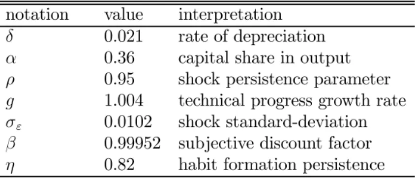
As stated by Table 1, which summarizes the calibration procedure, the values are,
{0.82, 0.99952, 0.0102} (12)
These estimates are quite standard: the habit parameter is close the value reported by Jermann (1998) and Boldrin, Christiano and Fisher (2001). The standard deviation of the shock is near to one percent which is quite acceptable.
3
Results
Given the calibration procedure we will organize our comments in two steps. Let us start by analyzing the implications on asset returns stylized facts. A general result is that the time-to-plan model provides a good explanation for asset returns facts (Table 2). The theoretical mean risk-free rate equals 1.79%. The empirical equity premium is well accounted for (6.04%
against 6.01% in the data). The capital gain effect is quite significative since the equity return volatility is 14.40% against 15.8% in the observed data.
What are the implications for the business cycle ? We analyze the model’s behavior in re-producing the second order moments of the cyclical components of consumption, investment employment and output. The cyclical component is obtained by applying the HP filter on the logged series. The relative volatility of investment is pretty good, whereas consumption’s volatility is understated. This is due to the habit formation which reduces the consumption volatility. The habit persistence, as a necessary condition to reproduce the empirical equity premium implies a volatility of consumption which is too low . For employment, the relative volatility is overstated. We conclude that the model performance in explaining the variable volatilities remains very average.
The model works better at reproducing the comovement of output with its components. The strength and the sign of the instantaneous correlation with output are close to their empirical counterpart. A salient result concerns the correlation between output and em-ployment. Empirically this correlation is 0.79. The model predicts 0.69 which means labor is perfectly procyclical. On this dimension, the time-to-plan model avoid one of the main criticism formulated against the capital adjustment cost mechanism, which predicts that employment is countercyclical.
Some counterfactual results must be indicated. The risk-free rate is too volatile compared to the empirical data. Finally, while the model heavily overestimates the persistence of the consumption growth rate (due to the habit formation in consumption) it turns out to be completely unable to generate the degree of persistence observed in the output growth rate.
Conclusion
The time-to-plan mechanism associated with habit formation constitutes a decisive step for-ward in the integrated analysis of business cycle and asset returns. This model provides a satisfactory explanation of asset returns when labour supply is endogenous. The main correlations with the output component are satisfactingly reproduced, particularly the in-stantaneous correlation between output and employment.
References
Blanchard, O. and Kahn, C. (1980). The solution of linear difference models under rational expectations. Econometrica, 48(5):1305—1311.
Boldrin, M., Christiano, L. J., and Fisher, J. D. M. (1995). Asset pricing lessons for modeling business cycles. NBER Working Paper, 5262.
Boldrin, M., Christiano, L. J., and Fisher, J. D. M. (2001). Habit persistence, asset returns and the business cycle. American Economic Review, 91(1):149—166.
Christiano, L. J. (2002). Solving dynamic equilibrium models by a method of undetermined coefficients. Computational Economics, 20:21—55.
Christiano, L. J. and Todd, R. M. (1996). Time to plan and aggregate fluctuations. Federal Reserve Bank of Mineapolis Quarterly Review, 20(1):14—27.
Christiano, L. J. and Vigfusson, R. J. (2002). Maximum likelihood in the frequency domain: The importance of time-to-plan. Journal of Monetary Economics, 50:789—815.
Kydland, F. E. and Prescott, E. C. (1982). Time to build and agregate fluctuations. Econo-metrica, 50:1345—1370.
Table 1. Parameters value notation value interpretation δ 0.021 rate of depreciation α 0.36 capital share in output ρ 0.95 shock persistence parameter g 1.004 technical progress growth rate σε 0.0102 shock standard-deviation
β 0.99952 subjective discount factor η 0.82 habit formation persistence
Table 2. Results
Asset returns Data Model
Mean value of
risk free rate 1.19 1.79
equity premium 6.01 6.04
Standard deviation of
risk free rate 1.41 4.30
return on equity 15.87 14.40
Sharpe Ratio 0.37 0.41
Business cycle Data Model
Relative standard deviation with output of
consumption 0.37 0.18
investment 2.15 2.62
employment 0.72 1.08
Correlation with output of
consumption 0.77 0.69
investment 0.91 0.99
employment 0.79 0.69
Persistence Data Model
Autocorrelation of the growth rate of
output 0.32 0.073