On the Relevance of the Bayesian Approach to Statistics
CHRISTIAN P. ROBERT
∗ †Universit´e Paris-Dauphine, CEREMADE, and CREST
In this essay, I argue about the relevance and the ultimate unity of the Bayesian approach in a neutral and agnostic manner. My main theme is that Bayesian data analysis is an effective tool for handling complex models, as proven by the increasing proportion of Bayesian studies in the applied sciences. I thus disregard the philosophical debates on the meaning of probability and on the random nature of parameters as things of the past that ultimately do a disservice to the approach and are irrelevant to most bystanders.
Keywords: Bayesian inference, Bayes model choice, foundations, testing, non-informative prior, Bayes factor, computational statistics
JEL Classifications: C11, C12, C13, C15, C44, C51, C52, C63
1
Introduction
Bayesian data analysis can be defined as a method for summarising uncertainty and making
estimates and predictions using probability statements conditional on observed data and an assumed model (Gelman 2008). In this essay, I aim to explain why I believe (with many others)
that Bayesian data analysis is valuable and useful in statistics, econometrics, and biostatistics, among other fields. My defence of the theme is based on presenting a user’s perspective and arguing in favour of the ultimate practicality of the Bayesian toolbox, whilst refraining from more elaborate philosophical and epistemological arguments on the nature of Science.
I do agree with Russell Davidson that the shrill tone of some – mostly past – defences of the Bayesian paradigm are doing it a disservice by transferring the debate to religious and therefore irrational grounds.1 My personal stance on the Bayesian choice is on the contrary grounded
in realism. The Bayesian perspective provides me with a complete toolbox that allows me to
∗
C.P. Robert is supported by the ANR-2009-BLAN-0318 “Big’MC” grant. He is grateful to the Bayesian Econometrics III workshop organisers for their invitation to lovely Rimini and for their support, and to Russell Davidson for such a congenial and open discussion. The editing help of Gael Martin over two successive versions greatly improved the presentation of this essay. Comments from Nicolas Chopin are also gratefully acknowledged.
†Email: [email protected] Webpage: xianblog.wordpress.com
1The barb of Russell Davidson, also found in Senn (2008), Bayesians are of course their own worst
enemies. They make non-Bayesians accuse them of religious fervour, and an unwillingness to see another point of view, is not completely unfounded.
c
2010 Christian P. Robert. Licenced under the Creative Commons Attribution-Noncommercial 3.0 Li-cence (http://creativecommons.org/licenses/by-nc/3.0/). Available at http://rofea.org.
conduct inference in an arbitrary setting at a minimal cost in terms of constructing statistical procedures. In addition, it provides sufficient theoretical safety rails to ensure coherence in my decision-making and convergence properties for my procedures. I also agree with Andrew Gelman’s (2008) reservation that a consequence of Bayesian statistics being given a proper
name is that it encourages too much historical deference from people who think that the bibles of Jeffreys, de Finetti, or Jaynes have all the answers. The formalisation of Bayesian statistics
by those pioneers has greatly contributed towards more efficiency in the design of Bayesian procedures (Robert et al. 2009) and therefore to their current popularity. However, naming a technique after particular scientists, even when as prestigious as those above, is a rhetorical trick to bring more authority to an approach. To keep the tone of this essay as clear as possible, I will nonetheless use the recent (Fienberg 2006) adjective of “Bayesian” in the following but I will mostly refrain from giving a name to alternatives, the usual adjective of “frequentist” seeming now out-dated and overly restrictive. The range of non-Bayesian statistical techniques indeed extends much further than looking at average properties.
As already done in the above, throughout the text I will be making (an admittedly selective) use of recent quotes that defend or criticise the Bayesian approach. Most of them emanate from a debate run by Bayesian Analysis following the tongue-in-cheek critique of Gelman (2008). I will present here elements to support Gelman’s (2008) conclusion that, given the advances in
practical Bayesian methods in the past two decades, anti-Bayesianism is no longer a serious option. My view is that denying the relevance of Bayesian analysis on the sole ground that it is
Bayesian does not follow from a rational stance.
2
Bayesian Models
Let me first stress that the Bayesian approach to non-parametrics is alive and well, as shown for instance by the recent advances in Dirichlet models (Teh et al. 2006) and Bayesian asymptotics (Ghosal and Van der Vaart 2006) (see also Hjort et al. 2009). Bayesian non-parametrics can now manage density and functional estimation with the same degree of complexity with which a normal mean is estimated by a Bayesian analysis based on a conjugate prior (Holmes et al. 2002). As regards Russell Davidson’s first question related to the Bahadur-Savage impossibility theorem, I do not understand the statistical point of the test in his Section 3 and I therefore have no answer. (His Theorem 1 reminds me very much of a result of the late Costas Goutis, reported in my book, Robert 2001, Table 3.2.3, about the range of Bayes estimators.) On the other hand, the issue raised by Russell Davidson in Section 7 about incorporating smoothness in the prior does not seem to be particularly problematic, once smoothness is defined in terms of a particular class of functions.
I will only consider here parametric settings, mostly for simplicity and space reasons. (And also for the fact that the priors found in non-parametric settings seem to be much more ac-ceptable as working tools by non-Bayesians.) The common ground for both parametric and
non-parametric settings is nonetheless that a model provides a likelihood. I simply do not be-lieve meaningful inference is possible without this likelihood function.2
Given that all models are approximations of the real world, the choice of a parametric model obviously is wide-open to criticism. As stated by Gelman (2008), Bayesians promote the idea
that a multiplicity of parameters can be handled via hierarchical, typically exchangeable, mod-els, but it seems implausible that this could really work automatically [instead of] giving rea-sonable answers using minimal assumptions. This is, however, a type of criticism that goes
beyond Bayesian modelling per se and questions the relevance of completely built models for drawing inference or running predictions. (Obviously, embracing my “opponent’s” perspective that inference is sometimes impossible would immediately close the discussion!) The Bayesian paradigm does not state that the model with which it operates is the “truth”, no more than it requires that the corresponding prior distribution has a connection with the “true” production of parameters (since there may even be no parameter at all). It simply provides an inferential machine that has strong optimality properties under the right model and that can similarly be evaluated under any other well-defined alternative models. In Popper’s (1934) terms, a Bayesian model can be “falsified” when faced with data from another model.3Templeton (2008) sees the
fact that having a high relative [posterior] probability does not mean that a hypothesis is true
or supported by the data as the ultimate drawback of the Bayesian paradigm. On the contrary,
I see it as a strength, even in Popperian terms, because (a) there is no such thing as a “true” hy-pothesis and (b) the support brought by the data is always relative to a reference model. Besides, the Bayesian approach is such that techniques allow prior beliefs to be tested and discarded as
appropriate (Gelman 2008). In other words, Bayesian data analysis has three stages: formu-lating a model, fitting the model to data, and checking the model fit (Gelman 2008). Hence,
there seems to be little reason for not using a parametric model at an early stage even if it is later dismissed as “not true enough” (in favour of another model).
Besides giving the Bayesian paradigm his name, Thomas Bayes contributed by stating the
definition of a conditional probability and deriving what is now known as Bayes theorem.4
Nonetheless, if surprisingly, there still exists a debate about the very nature of Bayes theorem.
2Of course, this statement goes against a large portion of the current practice that contends that first
moments are sufficient descriptions of the real world. But I do prefer the facilities provided by a full if wrong model to the adhocqueries required by a minimalist modelling. In particular, replying to Russell Davidson’s question in Section 4, I do not think there is a Bayesian approach to GMM’s unless one is ready to use a pseudo-likelihood that encompasses the specified moments.
3This is not to imply that the philosophy of Popper (1934) is in agreement with the Bayesian approach,
since Popper and Miller (1983) demonstrates the impossibility of coherent statistical inference.
4As stressed by Jaynes (2003), Bayes’ contribution to inference was essentially restricted to a somewhat
dubious toy example of locating the position of a billiard ball. In contrast, Laplace and others had a much wider range of examples, with more realistic applications. Jeffreys, de Finetti and Jaynes set the bases into firmer mathematical and methodological ground, while Wald and Stein established the fundamental optimality properties validating Bayes procedures.
Russell Davidson points out that it is difficult to express it in the formalism that is used in
fi-nancial economics/econometrics. Another illustration is given by Templeton (2008). He argues
that conditioning upon the observation x ∼ f (x|θ) is plainly invalid: The impact of treating x as
a fixed constant is to increase statistical power as an artefact and ignoring the sampling error of x undermines the statistical validity of all inferences made by the method. As validated by
standard measure theory (Billingsley 1986), the posterior distribution
π(θ|x) = R f (x|θ)π(θ)
f (x|θ)π(θ) dθ
does include the sampling (or error) distribution while conditioning on the data x. This ap-proach furthermore is the only coherent way to give a meaning to statements likeP(θ > 0|x), i.e. to properly construct confidence and prediction statements, while conditioning on the data at hand.5
Gelman (2008) reports that Bayesian methods are presented as an automatic inference
en-gine, and this raises suspicion in anyone with applied experience. It is true that π(θ|x) is the
core of Bayesian inference. It can legitimately be viewed as the “ultimate inference engine” via which all decisions (in a decision-theoretic framework) based on the data can be automati-cally derived. There is no fundamental difficulty in this automated derivation.6Once optimality criteria are explicitly stated via the utility function associated with the decision, searching for the optimal decision reduces to solving a well-posed optimisation problem.7 Furthermore, the
inference [step] gets most of the attention, but the Bayesian procedure as a whole is not auto-matic (Gelman 2008). In addition, using a probability distribution on the parameter space and
Bayes theorem allows for a coherent update of the information available on θ in the sense that the current posterior distribution becomes the prior distribution before gathering more data.
3
On Prior Selection
The recurrent criticism of the Bayesian perspective is that the whole inferential approach is ulti-mately dependent upon the choice of the prior distribution, as clearly shown by the definition of
5This point relates to Russell Davidson’s questions about the bootstrap. While I appreciate very much the
strength of bootstrapping techniques and find them a natural entry to Statistics for my third year students, I have trouble reconciliating the bootstrap and Bayesian statistics. Indeed, the bootstrap is fundamentally a plug-in method, especially in its parametric version, which therefore omits to properly take into account the variability of the plugged-in parameter estimates.
6That it is an automatic engine is an argument rarely advanced by critics of the Bayesian approach, who
on the contrary uniformly point out its subjective features. See Section 3.
7Gelman (2008) stresses that loss functions [are] not relevant to statistical inference and he does not
see any role for squared error loss, minimax, or the rest of what is sometimes called statistical decision theory. Following the arguments advanced in Robert (2001), but also in Berger (1985) and Bernardo and Smith (1994), I cannot but strongly disagree with this perspective. Decision theory is a strong motivation for using Bayesian procedures, especially in economics and econometrics where rationality is customarily associated with maximising utility functions.
the posterior distribution above. There is no possible debate about this fact, either from a math-ematical or methodological perspective. It is also straightforward to come up with examples where the choice of the prior leads to absurd decisions.
There is no easy answer to this criticism, but this acknowledgement must not be taken as conceding defeat in the debate! If the prior had no impact on the inference, data would be similarly useless, since the update would not matter. Therefore, I see this dependence as a plus of the Bayesian approach. It allows one to include an infinite range of prior opinions and items of information, while progressively concentrating on neighbourhoods of the “true” value of the parameter – in settings where the data is generated from the assumed model. In the literature, this point about the advantages of incorporating prior information is rather universally accepted. The criticisms instead focus on the opposite situation where the prior information is poor or inexistent, denying non-informative (or ignorance) priors their label, i.e. the representation of a state of complete ignorance.
Maybe surprisingly (and maybe not!), I completely agree with this criticism in that any choice of prior distribution corresponds to some informational input about the parameter. The ultimate argument is that, were there such a thing as the non-informative prior, it would be
expected to represent total ignorance about the problem (Kass and Wasserman 1996). Thus,
being moderately unfair (!), this object should be such an information black hole as to cancel the effect of any amount of information and should thus remain the same even after observing the data! Therefore, when Jeffreys (1939) states that if the parameter may have any value from
−∞to +∞, its prior probability should be taken as uniformly distributed, he is making a choice
of a particular structure of the model that impacts on his future inference, in addition to using the term uniform in an implicitly generalised manner because the parameter space is then un-bounded (Robert et al. 2009). Instead, as stated by Gelman (2008), there is no good objective
principle for choosing a noninformative prior (even if that concept were mathematically defined, which it is not). The notions of objective and of non-informative are indeed not well-defined
mathematical concepts and they carry an irrational undertone that fails to lend legitimacy to the associated priors. Some mathematical criteria do lead to some competing families of
ref-erence priors like the left Haar measures mentioned by Russell Davidson or matching priors
(see Robert 2001, Chapters 3 and 8). The ultimate attempt at producing a meaningful rationale for building non-informative priors is, in my opinion, Bernardo’s (1979) definition through the information theoretical device of Kullback divergence (see also Berger and Bernardo 1992). Quite obviously, this is not the only possible approach. Among other things, it depends on a choice of information measure, does not always lead to a solution and requires an ordering of the model parameters that involves some prior information (or some subjective choice). How-ever, as long as we do not think of those reference priors as representing ignorance (Lindley 1971), they can indeed be taken as reference priors, upon which everyone could fall back when
Apart from the conceptual confusion about non-informative priors that plagued most of the 19th and mid 20th century debate about the nature of Bayesian inference, the issue of improper priors often serves as a further criticism. Indeed, non-informative priors often are measurable functions π(θ) with infinite mass,
Z
Θ
π(θ) dθ = +∞ ,
which deprives them of a probabilistic interpretation. This criticism can be most easily rebutted for a wide variety of reasons. The first reason is topological coherence: limits of Bayesian procedures often partake of their optimality properties (Wald 1950) and should therefore be included in the range of possible procedures. Another one is robustness: a measure with an infinite mass is much more robust than a true probability distribution with a large variance.
Provided Z Θ f (x|θ)π(θ) dθ < ∞ , the quantity π(θ|x) = R f (x|θ)π(θ) Θf (x|θ)π(θ) dθ
is as well-defined as a probability density as a regular posterior distribution (Hartigan 1983, Berger 1985, Robert 2001).
4
Testing Versus Model Comparison
The inferential problems of Bayesian model selection and of Bayesian testing are clearly those for which the most vigorous criticisms can be found in the literature. An illustration is provided by Senn (2008) who states that the Jeffreys-subjective synthesis betrays a much more dangerous
confusion than the Neyman-Pearson-Fisher synthesis as regards hypothesis tests. I find this
suspicion rather intriguing given that the Bayesian approach is the only one giving a proper meaning to the probability of a null hypothesis,P(H0|x). Alternative methodologies are able, at
best, to specify a probability value on the sampling space, i.e. on the “wrong” space since the only variation is on the parameter space once the observation is obtained.
Senn (2008) further advances that what is almost never used, however, is the Jeffreys
sig-nificance test. I recall here that the most standard Bayesian approach to testing and model
choice relies on the Bayes factor (Kass and Raftery 1995), which, for hypotheses written as
H0 : θ ∈ Θ0and as H1 : θ ∈ Θ1, is defined as (Jeffreys 1939, Jaynes 2003)
B01= π(Θ0|x) π(Θ1|x) π(Θ 0) π(Θ1) = Z Θ0 f (x|θ)π0(θ)dθ Z Θ1 f (x|θ)π1(θ)dθ .
This monotonic transform of the posterior probability of H0eliminates the influence of the prior
not suffer from the over-fitting difficulties of the latter, in that it includes a natural penalisation factor for richer models. This is shown by the connection with the BIC (Bayesian information criterion), intuited by Jeffreys (1939): variation is random until the contrary is shown; and
new parameters in laws, when they are suggested, must be tested one at a time, unless there is specific reason to the contrary. Although I strongly dislike using the term because of its
undeserved weight of academic authority, the Bayes factor acts as a natural Ockham’s razor. A criticism of the use of Bayes factors (e.g., Templeton 2008) is that the quantity is not scaled in probability terms. On the contrary, I maintain it is naturally scaled against one and can, moreover, be readily transformed into posterior probabilities when the prior probabilities of the hypotheses are specified. (It is furthermore a natural factor in a decision-theoretic framework, see Robert 2001.) Another criticism is rarely voiced outside the Bayesian community, namely that the use of improper priors is mostly prohibited in this setting, for lack of proper normalising constants. Solutions have been proposed, akin to cross-validation techniques in the classical domain (Berger and Pericchi 1996, Berger et al. 1998), but they are somehow too ad-hoc to convince the entire community (and obviously beyond).
If we consider the special case of point null hypotheses – which is not so limited in scope since it includes all variable selection setups – there is a difficulty with using a standard prior in this environment. As put by Jeffreys (1939), when considering whether a location parameter
αis 0 [when] the prior is uniform, we should have to take π(α) = 0 and B10would always be
infinite. This is a case when the inferential question implies a modification of the prior, justified
by the information contained in the question. Avoiding the whole issue is a clear-cut solution, as with Gelman (2008) having no patience for statistical methods that assign positive probability
to point hypotheses of the θ = 0 type that can never actually be true. Considering the null and
the alternative hypotheses as defining two different models is another solution that allows for a Bayes factor representation.
A major criticism directed at the Bayesian approach to testing is that it is not interpretable on the same scale as the Neyman-Pearson-Fisher solution, namely in terms of Type I error prob-ability and test power. In other words, frequentist methods have coverage guarantees; Bayesian
methods don’t; 95 percent frequentist intervals will live up to their advertised coverage claims
(Wasserman 2008). A natural thing to do is then to question the appeal of such frequentist prop-erties when considering a single dataset. That is, in Jeffreys’ (1939) famous words, a hypothesis
that may be true may be rejected because it had not predicted observable results that have not occurred. From a decision-theoretic perspective – to which the frequentist properties should
relate – a classical Neyman-Pearson-Fisher procedure is never evaluated in terms of the con-sequences of rejecting the null hypothesis, even though the rejection must imply a subsequent action towards the choice of an alternative model. (From a narrower decision-theoretic perspec-tive, note also that p-values may be inadmissible estimators, Hwang et al. 1992.) Therefore, arguing that high posteriors probabilities do not imply that a hypothesis is true as in Templeton
(2008) and that the Bayesian approach is relative in that it posits two or more alternative
hy-potheses and tests their relative fits to some observed statistics (Templeton 2008), is missing the
main purpose of Bayesian tests. Bayesian procedures do not aim at validating or invalidating a golden model per se but rather lead to the choice of a working model that allows for acceptable predictive properties.8
Another criticism covers the lack of asymmetry of the Bayes factor, since it satisfies the equality B10= 1/B01. For model choice, i.e. when several models are under comparison for the
same observation
Mi: x ∼ fi(x|θi) , i ∈I,
whereIcan be finite or infinite, this symmetry seems to me to be a fundamentally sound
prop-erty. Nevertheless, Templeton (2008) bemoans that there is no null hypothesis, which
compli-cates the computation of sampling error, since there is no single statistical model under which to evaluate sampling. This should be construed as a clear limitation of the
Neyman-Pearson-Fisher paradigm, since the latter imposes asymmetry and (Type I) error control under a single (null) model. However, this is not the perspective of Templeton (2008) who concludes with the impossibility of the posterior probability of a model,
π(Mi|x) = pi Z Θi fi(x|θi)πi(θi)dθi X j pj Z Θj fj(x|θj)πj(θj)dθj
due to the impression that the numerators are not co-measurable across hypotheses, and the
denominators are sums of non-co-measurable entities. Hence, the “posterior probabilities” that emerge are not co-measurable. This means that it is mathematically impossible for them to be probabilities. Given that all terms are marginal likelihoods for the same observation, it
seems difficult to argue against their co-measurability. Contrary to classical plug-in likelihoods, marginal likelihoods do allow for a comparison on the same scale. Similarly, the belief that
complicating dimensionality of test statistics is the fact that the models are often not nested, and one model may contain parameters that do not have analogues in the other models and vice versa (Templeton 2008) is not well-founded. The Bayes factor is properly defined and
applicable to settings where the models are not embedded (or nested). This is due to the fact that the corresponding quantity of interest for a given model is the marginal likelihood (or evidence), which integrates over spaces and complexity and which can be interpreted at face value since it is calibrated across models.
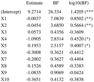
A last point of contention about Bayesian testing is the apparent absence of clearly defined directions when conducting a standard analysis. Figure 1 reproduces an output from Marin and
8It is worth repeating the earlier assertion that all models are false and that finding that a hypothesis is
Robert (2007b). This computer output illustrates how a default prior and Bayes factors can be used in the same spirit as significance levels in a standard regression model, each Bayes factor being associated with the test of the nullity of the corresponding regression coefficient. This output mimics the standardR function lm outcome in order to show that the level of information provided by the Bayesian analysis goes beyond the classical output. My point here is obviously not in showing that we can get similar answers to those of a least square analysis since, else, we might as well use the frequentist method (Wasserman 2008). It is to demonstrate that reference analyses are available, while preserving the strength of the Bayesian machinery (like joint confidence regions and multiple tests).
Figure 1:Routput of a Bayesian regression on a processionary caterpillar dataset with ten covariates analysed in Marin and Robert (2007b).
Estimate BF log10(BF) (Intercept) 9.2714 26.334 1.4205 (***) X1 -0.0037 7.0839 0.8502 (**) X2 -0.0454 3.6850 0.5664 (**) X3 0.0573 0.4356 -0.3609 X4 -1.0905 2.8314 0.4520 (*) X5 0.1953 2.5157 0.4007 (*) X6 -0.3008 0.3621 -0.4412 X7 -0.2002 0.3627 -0.4404 X8 0.1526 0.4589 -0.3383 X9 -1.0835 0.9069 -0.0424 X10 -0.3651 0.4132 -0.3838
evidence against H0: (****) decisive, (***) strong, (**) substantial, (*) poor
5
On Pervasive Computing
Bayesian analysis has long been derided for providing optimal answers that could not be com-puted. With the advent of early Monte Carlo methods, of personal computers, and, more re-cently, of more powerful Monte Carlo methods (Hitchcock 2003), the pendulum appears to have switched to the other extreme. Nowadays, Bayesian methods seem to quickly move to elaborate
computation (Gelman 2008). This feature does not make Bayesian methods less suspicious
in the mind of critics for different reasons: a simulation method of inference hides unrealistic
assumptions (Templeton 2008). I won’t launch here into a defence of simulation techniques
that have done so much to promote Bayesian analysis in the past decades, referring to Chen et al. (2000), Robert and Casella (2004), Marin and Robert (2007b) for detailed arguments and to
Robert and Marin (2010), Robert and Wraith (2009) for specific coverages of the computational advances related to Bayesian model choice. Simulation methods can certainly be misused, as any methodology can be. However, while Bayesian simulation [may seem] stuck in an infinite
regress of inferential uncertainty (Gelman 2008), there exist enough convergence assessment
techniques (Robert and Casella 2010) to ensure a reasonable degree of confidence in the accu-racy of the approximation provided by those simulation methods. Thus, as rightly stressed by Bernardo (2008), the discussion of computational issues should not be allowed to obscure the
need for further analysis of inferential questions.9
In Section 6, Russell Davidson asks about the reliability of Markov chain Monte Carlo (MCMC) methods and about recent developments in this field. The answer is more complex than time and space allow in this essay, so my first reply is to refer him to (Robert and Casella 2004, 2009) for booklength entries. A second response is that, despite their specific label, MCMC methods do not differ in essence from other Monte Carlo methods. When using an im-portance sampler or an harmonic mean estimator (see Marin and Robert 2007a for details), the quantities we produce are unbiased, which is not a characteristic of MCMC outputs. However, they may also be associated with infinite variance, which means that their convergence time is beyond anyone’s patience! The same applies to MCMC samples which are formally associated with the correct stationary distribution but which may in practice end up with a cosmologi-cal number of iterations! Robert and Casella (2010) details several tools that help in checking convergence and stationarity, but those tools are not completely foolproof. Therefore it may happen that the lack of convergence of a MCMC output remains undetected. Similarly, using a numerical integration software may fail to detect an important region for the integrand. Those are numerical problems that have little to do with the methodology under scrutiny and can often be detected by using a multifaceted strategy, mixing together several numerical methods.
Interestingly enough, the most accurate – in our opinion – approximation technique for Bayes factors is, when applicable, derived from Bayes theorem. This is indeed the purpose of Chib’s (1995) rendering:
m(x) = π(θ) f (x|θ)
π(θ|x) ≈
π(θ) f (x|θ) ˆπ(θ|x) ,
where ˆπ(θ|x) is a simulation-based approximation to the posterior density. Marin and Robert (2008) propose an illustration in the setting of mixtures, while Robert and Marin (2010) im-plement the method for a probit model, with both examples demonstrating the precision of this approximation. There have been discussions about the accuracy of this method in multimodal settings (Fr¨uhwirth-Schnatter 2004), but straightforward modifications (Berkhof et al. 2003, Lee
9The confusion of Templeton (2008) is of this nature, namely his criticisms bear in fact on the generic
principles of Bayesian inference and in particular testing while he aims at criticising a specific simulation methodology called ABC and described below. See Beaumont et al. (2010) for a discussion of this confusion.
et al. 2008) overcome such difficulties and make for both an easy and a robust computational tool associated with Bayes factors.
Instead of presenting the whole range of available computational solutions, I want to point out here a single but recent advance in Bayesian computing that allows for a further extension of Bayesian data analysis to cases where any other method of inference is either impossible or seriously inaccurate. This new method is called ABC, standing for Approximate Bayesian
Computation. It was introduced in genomics by Pritchard et al. (1999) to handle models, like
phylogenic trees, where the likelihood could not be computed in a reasonable time, hence pro-hibiting the use of standard simulation tools. The method is based on a standard accept-reject principle generating θ ∼ π(θ), x′∼ f (x|θ) until x′= x which produces a generation from π(θ|x).
Since the stopping rule is impossible to attain in continuous settings, the approximation in ABC consists in replacing x = x′with a relaxed condition, d(x, x′) < ǫ, where d is an arbitrary di-vergence measure and ǫ is an approximation parameter to be calibrated. Assuming that new “observations” x′from the likelihood can be easily simulated, this method provides controlled approximations π(θ|d(x, x′) < ǫ) to the posterior distribution. The accuracy of this method
can be calibrated against the available computing power and it is currently in standard use for genomic applications (Cornuet et al. 2008) as well as for model choice in graphical models (Grelaud et al. 2009).10
The field of Bayesian computing is therefore very much alive and, while its diversity can be construed as a drawback by some, I do see the emergence of new computing methods adapted to specific applications as most promising, because it bears witness to the growing involvement of new communities of researchers in Bayesian advances.
6
Conclusion
Once again, I want to stress that the purpose of this essay is far from trying to preach in favour of my creed, as I do not see Bayesian data analysis as a philosophical (and even less reli-gious) stance. What drives my Bayesian choice is the essential practicality of the tools and of the actions I can undertake thanks to that choice, as well as the ability to evaluate, criti-cise, and possibly modify, the calibration choices I have made at the beginning of my analysis. There is beauty as well as efficiency in transparency and a Bayesian data analysis is ultimately transparent in that it displays all of its components (prior, likelihood, loss function, simulation technique) for public evaluation. The fact that any of these components can be replaced by an alternative version explains and illustrates the versatility of the method and the appeal it exerts on non-statisticians in need of a data analysis tool. The other practical side of Bayesian data analysis is that we now see a growing range of complex models where, apart from abdicating
10(Grelaud et al. 2009) is one illustration of the high popularity of Bayesian techniques in epidemiology,
biostatistics and genomics. I thus disagree with Russell Davidson’s impression of the opposite at the end of Section 8!
on some part of the complexity, the only available solution is to use a Bayesian approach. Han-dling highly non-identifiable models, inferring about the graphical structure of a spatial model, running a small area estimation on an very dense grid, analysing continuous time data with hidden Markov structures, all of these problems and a myriad of others cannot be processed but from a Bayesian perspective.
References
Beaumont, M., Nielsen, R., Robert, C., Hey, J., Gaggiotti, O., Knowles, L., Estoup, A., Ma-hesh, P., Coranders, J., Hickerson, M., Sisson, S., Fagundes, N., Chikhi, L., Beerli, P., Vitalis, R., Cornuet, J.-M., Huelsenbeck, J., Foll, M., Yang, Z., Rousset, F., Balding, D. and Excoffier, L. (2010), In defense of model-based inference in phylogeography, Molecular
Ecology 19(3), 436–446.
Berger, J. (1985), Statistical Decision Theory and Bayesian Analysis, second edn, Springer-Verlag, New York.
Berger, J. and Bernardo, J. (1992), On the development of the reference prior method, in J. Berger, J. Bernardo, A. Dawid and A. Smith (eds), Bayesian Statistics 4, Oxford Uni-versity Press, London, pp. 35–49.
Berger, J. and Pericchi, L. (1996), The Intrinsic Bayes Factor for Model Selection and Predic-tion, J. American Statist. Assoc. 91, 109–122.
Berger, J., Pericchi, L. and Varshavsky, J. (1998), Bayes factors and marginal distributions in invariant situations, Sankhya A 60, 307–321.
Berkhof, J., van Mechelen, I. and Gelman, A. (2003), A Bayesian approach to the selection and testing of mixture models, Statistica Sinica 13, 423–442.
Bernardo, J. (1979), Reference posterior distributions for Bayesian inference (with discussion),
J. Royal Statist. Society Series B 41, 113–147.
Bernardo, J. (2008), Comment on Article by Gelman, Bayesian Analysis 3(3), 451–454. Bernardo, J. and Smith, A. (1994), Bayesian Theory, John Wiley, New York.
Billingsley, P. (1986), Probability and Measure, second edn, John Wiley, New York.
Chen, M., Shao, Q. and Ibrahim, J. (2000), Monte Carlo Methods in Bayesian Computation, Springer-Verlag, New York.
Chib, S. (1995), Marginal likelihood from the Gibbs output, J. American Statist. Assoc.
90, 1313–1321.
Cornuet, J.-M., Santos, F., Beaumont, M. A., Robert, C. P., Marin, J.-M., Balding, D. J., Guille-maud, T. and Estoup, A. (2008), Inferring population history with DIYABC: a user-friendly approach to Approximate Bayesian Computation, Bioinformatics 24(23), 2713–2719. Fienberg, S. (2006), When did Bayesian inference become “Bayesian”?, Bayesian Analysis
1(1), 1–40.
switching models using bridge sampling techniques, The Econometrics Journal 7(1), 143– 167.
Gelman, A. (2008), Objections to Bayesian statistics, Bayesian Analysis 3(3), 445–450. Ghosal, S. and Van der Vaart, A. (2006), Convergence rates of posterior distributions for non
iid observations, Ann. Statist. 35(1), 192–223.
Grelaud, A., Marin, J.-M., Robert, C., Rodolphe, F. and Tally, F. (2009), Likelihood-free meth-ods for model choice in Gibbs random fields, Bayesian Analysis 3(2), 427–442.
Hartigan, J. A. (1983), Bayes Theory, Springer-Verlag, New York, New York.
Hitchcock, D. H. (2003), A History of the Metropolis–Hastings Algorithm, The American
Statistician.
Hjort, N., Holmes, C., M¨uller, P. and Walker, S. (2009), Bayesian Nonparametrics: Principles
and Practice, Cambridge University Press, Cambridge, UK.
Holmes, C., Denison, D., Mallick, B. and Smith, A. (2002), Bayesian methods for nonlinear
classification and regression, John Wiley, New York.
Hwang, J., Casella, G., Robert, C., Wells, M. and Farrel, R. (1992), Estimation of accuracy in testing, Ann. Statist. 20, 490–509.
Jaynes, E. (2003), Probability Theory, Cambridge University Press, Cambridge. Jeffreys, H. (1939), Theory of Probability, first edn, The Clarendon Press, Oxford. Kass, R. and Raftery, A. (1995), Bayes factors, J. American Statist. Assoc. 90, 773–795. Kass, R. and Wasserman, L. (1996), Formal rules of selecting prior distributions: a review and
annotated bibliography, J. American Statist. Assoc. 91, 343–1370.
Lee, K., Marin, J.-M., Mengersen, K. and Robert, C. (2008), Bayesian Inference on Mixtures of Distributions, in N. N. Sastry (ed.), Platinum Jubilee of the Indian Statistical Institute, Indian Statistical Institute, Bangalore.
Lindley, D. (1971), Bayesian Statistics, A Review, SIAM, Philadelphia.
Marin, J. and Robert, C. (2007a), Importance sampling methods for Bayesian discrimination between embedded models, in M.-H. Chen, D. Dey, P. M¨uller, D. Sun and K. Ye (eds),
Frontiers of Statistical Decision Making and Bayesian Analysis, Springer-Verlag, New York.
To appear, see arXiv:0910.2325.
Marin, J.-M. and Robert, C. (2007b), Bayesian Core, Springer-Verlag, New York.
Marin, J.-M. and Robert, C. (2008), Approximating the marginal likelihood in mixture models,
Bulletin of the Indian Chapter of ISBA V(1), 2–7.
Popper, K. (1934), The Logic of Scientific Discovery, London: Hutchinson and Co. (English translation, 1959).
Popper, K. and Miller, D. (1983), The Impossibility of Inductive Probability, Nature 310, 434. Pritchard, J. K., Seielstad, M. T., Perez-Lezaun, A. and Feldman, M. W. (1999), Population
growth of human Y chromosomes: a study of Y chromosome microsatellites, Mol. Biol.
Robert, C. (2001), The Bayesian Choice, second edn, Springer-Verlag, New York.
Robert, C. and Casella, G. (2004), Monte Carlo Statistical Methods, second edn, Springer-Verlag, New York.
Robert, C. and Casella, G. (2009), Introducing Monte Carlo Methods with R, Springer-Verlag, New York.
Robert, C. and Casella, G. (2010), A History of Markov Chain Monte Carlo-Subjective Rec-ollections from Incomplete Data, in S. Brooks, A. Gelman, X. Meng and G. Jones (eds),
Handbook of Markov Chain Monte Carlo: Methods and Applications, Chapman and Hall,
New York. arXiv0808.2902.
Robert, C. and Marin, J.-M. (2010), Importance sampling methods for Bayesian discrimination between embedded models, in M.-H. Chen, D. K. Dey, P. Mueller, D. Sun and K. Ye (eds),
Frontiers of Statistical Decision Making and Bayesian Analysis, Springer-Verlag, New York.
(To appear.).
Robert, C. and Wraith, D. (2009), Computational methods for Bayesian model choice, in P. M. Goggans and C.-Y. Chan (eds), MaxEnt 2009 proceedings, Vol. 1193, AIP.
Robert, C., Chopin, N. and Rousseau, J. (2009), Theory of Probability revisited (with discus-sion), Statist. Science. (to appear).
Senn, S. (2008), Comment on Article by Gelman, Bayesian Analysis 3(3), 459–462.
Teh, Y. W., Jordan, M. I., Beal, M. J., and Blei, D. M. (2006), Hierarchical Dirichlet Processes,
J. American Statist. Assoc. 101, 1566–1581.
Templeton, A. (2008), Statistical hypothesis testing in intraspecific phylogeography: nested clade phylogeographical analysis vs. approximate Bayesian computation, Molecular
Ecol-ogy 18(2), 319–331.
Wald, A. (1950), Statistical Decision Functions, John Wiley, New York.