lq-regularization of the Kalman filter for exogenous outlier removal: application to hedge funds analysis

Electronic copy available at: http://ssrn.com/abstract=1949678

l

q

-regularization of the Kalman Filter for exogenous

outlier removal: application to hedge funds analysis

Emmanuelle Jay

_{, Patrick Duvaut}

_{, Serge Darolles}

_{and Christian Gouri´eroux}

⇤_{QAMLAB, Palais Brongniart, 28 Place de la Bourse, 75002 Paris, France, Email: [email protected]} †_{ETIS/CNRS UMR 8051, 6 av. du Ponceau, 95014 Cergy-Pontoise Cedex, France, Email: [email protected]}

‡_{CREST, 15 Bd Gabriel P´eri, 92245 Malakoff Cedex, France, Email: [email protected]} §_{QUANTVALLEY, Palais Brongniart, 28 Place de la Bourse, 75002 Paris, France}

Abstract—This paper presents a simple and efficient exoge-nous outlier detection & estimation algorithm introduced in a regularized version of the Kalman Filter (KF). Exogenous outliers that may occur in the observations are considered as an additional stochastic impulse process in the KF observation equation that requires a regularization of the innovation in the KF recursive equations. Regularizing with a l1_{- or l}2_{-norm needs}

to determine the value of the regularization parameter. Since the KF innovation error is assumed to be Gaussian we propose to first detect the possible occurrence of an exogenous impulsive spike and then to estimate its amplitude using an adapted value of the regularization parameter. The algorithm is first validated on synthetic data and then applied to a concrete financial case that deals with the analysis of hedge fund returns. The proposed algorithm can detect anomalies frequently observed in hedge returns such as illiquidity issues.

I. INTRODUCTION

Exogenous outlier removal is one of the most common problems encountered in processing real data. Outliers may come from unknown sensor failures, abnormal measurements or even intentional jamming. In the framework of tracking or estimating unobserved processes, usually solved with KF or one of its extensions, such exogenous outliers are referred to as additive outliers or AO’s [1], [2] and occur in the observation. Endogenous outliers that may affect the innovations of the state equation are called innovative outliers or IO’s and are out of the scope of this paper. Recursive least squares can serve to deal with AO’s applying a Huber weight function [3] to the innovation error in the KF recursive equation. One can also penalize the Kalman filter by introducing a l1_{- or l}2 -regularization term. Regularization usually offers good results but requires the determination of the regularization parameter introduced to limit the amplitude of the solution. The search for the optimal regularization parameter has no ideal solution and each existing method (e.g. cross-validation, generalized cross-validation, maximum a posteriori estimation, Bernoulli-Gauss assumption or MCMC methods) is fit to the problem under study. Regularization is widely used in statistical signal processing (e.g. in basis pursuit, compressed sensing, signal recovery, wavelet thresholding), in statistics with ridge regres-sions and LASSO algorithm or fused LASSO [4] and is also very useful in decoding linear codes or geophysics problems. In finance, l1_{-regularization is also leveraged in the context of} portfolio optimization [5], [6], [7].

The paper is organized as follows: section 3 presents the robust Kalman Filter (RKF) as described in [8]. The family of detection & estimation algorithms we introduce to handle exogenous outliers is presented in section 4 and section 5 is devoted to the application of our algorithm to detecting irreg-ularities in hedge funds returns. The sixth section concludes.

II. NOTATION

Uppercase and lowercase bold letters denote matrices and column-vectors, respectively. (.)0_{stands for transpose operator,} 0J for a J ⇥ J null matrix, IJ for a J ⇥ J identity matrix, N (µ, ⌃) for the multivariate Gaussian distribution with mean vector µ and covariance matrix ⌃, IE(.) for the mathematical expectation, V ar(.) for the variance, Cov(.) for the covari-ance, ||.||1 for the l1-norm, and ||.||2 for the l2-norm.

III. ROBUSTKALMANFILTER(RKF )

The Robust Kalman Filter (RKF) setup is as follows [8]:

✓t = ✓t 1+ !t, (1)

rt = g0t✓t+ vt+ ✏t. (2) ✓tis the unknown m-dimensional state vector to be estimated at each time step t, !t - the state noise - is N (0m, w2Im), rt is the observed value at time t, gt is a m-dimensional vector of observed variables, ✏t the observation noise -is N (0, 2

✏), and vt is a stochastic impulse process, e.g. a Bernoulli-Gaussian process, suited to model unknown sensor failures, measurement outliers or even intentional jamming. Parameters w and ✏ are supposed to be known and the observed variable rtis scalar.

As with the standard KF (where vt = 0), the objective of the problem stated in (1) and (2) is to derive recursive estimate ˆ✓t/t of the unobservable parameter ✓t, given the measurement rt and the observed variables gt up to time t, based on the minimization of the mean-square error (MSE) IE(|✓t ✓ˆt/t|2). In the presence of the non-Gaussian outlier vt, the optimum recursive estimate cannot be explicitly derived and moreover may be nonlinear. An elegant alternative consists in regularizing the KF quadratic cost function by adding a lq -penalty (l1 _{in RKF). The RKF algorithm goes through the}

Electronic copy available at: http://ssrn.com/abstract=1949678 following steps. The prediction step is the same as for the

standard KF and is given by: KF Prediction

ˆ

✓t/t 1 = ✓ˆt 1/t 1, (3) St/t 1 = St 1/t 1+ w2Im, (4) where St/t = Cov(✓t ˆ✓t/t) is the error covariance matrix of the estimates. To handle the additional term vt in (2), the recursive equations of the correction step are slightly modified. Given the innovation or measurement error:

˜

rt= rt g0t✓ˆt/t 1, (5) and the optimal Kalman gain:

zt= St/t 1gt(g0tSt/t 1gt+ ✏2) 1, (6) then, the correction equations are as follows:

Correction

St/t = (Im ztg0t) St/t 1, (7) ˆ

✓t/t = ✓ˆt/t 1+ zt(˜rt ˆvt). (8) In (8), the estimated value ˆvtis the solution of:

argmin vt C(vt, ) = min vt (˜rt vt)0qt(˜rt vt) + ||vt||1, (9) with qt = (1–gt0zt)0 ✏i2(1 g 0 tzt) + z0tSt/t 11 zt > 0 and 0being the regularization parameter.

Equation (9) is referred to as a regularized regression and is equivalent to the LASSO setup [4], [9]. Given an appropriate value of , minimizing C(vt, ) is equivalent to jointly detecting and estimating vt. The l1-norm will shrink the value of vt to zero for small values of and consider a nonzero value of vt with a high value of . Jointly detecting and estimating ˆvt relies therefore on the good choice of which has to be tuned such that the sparsity of vt coincides with the sparsity seen through the observations. If the value of is inappropriate then many false alarms are generated. In [4], the author observes that the search for can be restricted to the range [0, 2 qt|˜rt|]. In practice, the upper bound seems to be very generous [10], but it can be adaptive and specific to the observed variable.

IV. REGULARIZEDKALMANFILTER(rgKF) Hereafter, we propose a family of algorithms called the regularized Kalman Filter or rgKF(OD, E-lq_{) that includes} an Outlier Detection step (OD) followed by a lq _{(q > 0)} Estimation step (E-lq_{). OD stands for the name of the detection} method, e.g. if OD=NG then a Non-Gaussian deviation test is applied. In the following, we consider only q = 1, 2. The RKF in [8], which consists of a single and joint detection/estimation step, falls into the l1_{-regularization approach and is equivalent} to rgKF(l1_{, E-l}1_{). TABLE I sums up these algorithms.}

What we call the regularized Kalman Filter or rgKF is a simple and efficient algorithm. Based on the fact that vt is an additive outlier in the observations, it is obvious that

TABLE I

FAMILY OFOutlier Detection and EstimationALGORITHMS.

OD E-lq

RKF l1 _fixed

rgKF(NG, E-l1_{) NG l}1 _{2 [0, 2 q}

t|˜rt|]

rgKF(NG, E-l2_{) NG l}2 _fixed

the innovation ˜rt in (5) should contain vt if vt occurs at time t. Moreover, the observation error ✏t is assumed to be a Gaussian random variable with a fixed variance 2

✏. If vt occurs at time t, then ˜rt should not lie in the range space of the Gaussian density. Our rgKF algorithm with exogenous outlier detection & estimation can be summed-up in the four following steps:

rgKF(NG, E-lq_{), q = 1, 2} 1) KF Prediction

a) Computation of ˆ✓t/t 1 (3) and St/t 1 (4)

b) Computation of innovation (5) and Kalman Gain (6), 2) Outlier Detection

a) Prediction step of the mean and standard deviation of ˜

rt(for t > 2, with initial values ˆµ2/2= ˜r2and ˆ_2/22 = 0): ˆ µt/t 1 = t 1 t µˆt 1/t 1+ 1 tr˜t, (10) ˆ_{t/t 1}2 = t 2 t 1ˆ 2 t 1/t 1+ t (ˆµt/t 1 µˆt 1/t 1)2. (11) b) Non-Gaussian test: if |˜rt µˆt/t 1| > 3 ˆt/t 1 then an outlier is detected.

3) Outlier Estimation • if 2b) is verified: E-l1 _{case: set}

t= 10 2 and estimate ˆvtusing (9). E-l2 _{case: if the regularization term in (9) is ||v}

t||22 instead of ||vt||1 then estimate ˆvt,l2 is as follows:

ˆ vt,l2 = ˜ rtqt t,l2+ q_t . (12)

Note: by definition and following 2b), we should have |˜rt ˆvt,l2| < 3 _✏, so that _t,l2 should lie in the range



0, 3 ✏qt |˜rt| 3 ✏

• otherwise (if no detection) ˆvt= 0. 4) rgKF Correction

- The covariance matrix is updated using (7), - The state is updated according to (8),

- The mean of the innovation is updated as follows: ˆ

µt/t= ˆµt/t 1 1

tvˆt, (13) - The variance of the innovation becomes:

ˆ2 t/t= t 2 t 1ˆ 2 t 1/t 1+ t (ˆµt/t µˆt 1/t 1)2. (14)

V. APPLICATION TO DETECTING IRREGULARITIES IN

HEDGEFUNDS RETURNS

A. Definition and description of the problem

In the financial asset literature, (2) with vt = 0 is known as a multi-factor model (see [11] for more details) and is statistically interpreted as a linear regression with stochastic parameters. The returns rtof a risky asset are linked to some factors ft (in (2), gt=⇥1 ft0

⇤0 _{to include a constant term in} the regression and ✓t=

⇥ ↵t 0t

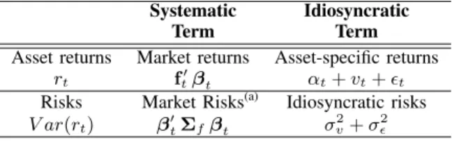
⇤0_{) which may be micro- or} macro-economic data, fundamental values, statistical factors or specific portfolios. These factors represent the various sources of risk present in the market to which an investor is exposed. The risks coming from the factors exposures t are called the systematic risks: they are common to all of the assets whose returns are expressed using (2) and cannot be lowered by diversification. Oppositely, the residual terms in (2) are totally specific to the assets and are related to the so-called idiosyncratic risks. They represent the part of the returns which cannot be explained by market factors but whose risks may be reduced with diversification. TABLE II gives an overview of the asset returns and risk break down.

TABLE II

BREAK DOWN OF ASSET RETURNS AND RISKS INTOsystematic

ANDidiosyncraticCOMPONENTS

Systematic Idiosyncratic Term Term Asset returns Market returns Asset-specific returns

rt ft0 t ↵t+ vt+ ✏t

Risks Market Risks(a) _{Idiosyncratic risks}

V ar(rt) 0t⌃f t

2 v+ ✏2 (a)_⌃

f is the covariance matrix of the factors.

The goal of our example is to explain the importance of removing outliers using rgKF algorithms. A multi-factor decomposition of the returns helps us to understand which part of the returns comes from the market and which one is specific. If outliers appear in the observations and if the model does not take them into account, then market exposures estimates can be totally spurious. rgKF algorithms avoid the contamination of these estimates by simply removing outliers. In practice, portfolio managers can use multi-factor approaches to hedge one specific or all market risks. Bad estimates can lead to take some inappropriate decisions concerning the optimal hedging portfolio. The tests are first conducted on synthetic data and then applied on real data.

B. Impact of outliers on synthetic returns

Synthetic returns are built with constant parameters ↵ = 0.02, 1 = 0.15 and 2 = 0.23, and two of the eight risk factors of Fung & Hsieh (F&H) [12], [13], the Standard and Poor’s 500 Index (S&P500, f1) and the Emerging Market index (MXEF, f2). A Gaussian noise is added to the resulting time series. A spiky version of these synthetic returns is also constructed (adding occurences of vt): we randomly chose three instants of arrival (being 30-Jun-2000, 31-Oct-2003 and 31-Dec-2007 on Fig. 1) on which spikes were randomly

generated as N (0, 0.5). Fig. 1 shows what happens on the

0.1 0.15 0.2 0.25 0.3 Theoretical KF KF when SPIKES 0.1 0.15 0.2 0.25 0.3 Theoretical RKF ( =0.5) RKF when SPIKES

Jan00 Jan05 Jan10

0.1 0.15 0.2 0.25 0.3 Theoretical rgKF(NG,l1 ) rgKF(NG,l1 ) when SPIKES

Jan00 Jan05 Jan10

0.1 0.15 0.2 0.25 0.3 Theoretical rgKF(NG,l2 ) rgKF(NG,l2 ) when SPIKES

Impact of outliers on the estimation of

2=0.23 ; Synthetic data with constant parameters

Fig. 1. Comparison of the impact of outliers present in the observations

on the estimation of 2 of the synthetic data between KF, RKF ( = 0.5),

rgKF(NG,l1_{) and rgKF(NG,l}2_{; = 0.5).}

estimated parameters of the model and compares four different estimation methods: KF, RKF with = 0.5,rgKF(NG,l1_{) and} rgKF(NG,l2_{) with = 0.5. We observe that without any} consideration for the possible occurrence of outliers in the observations (as for KF), parameter estimations become totally spurious and very far from the theoretical values. Inversely, rgKFs perform similarly with or without outliers and the results are also very close to the Kalman Filter results without outliers.

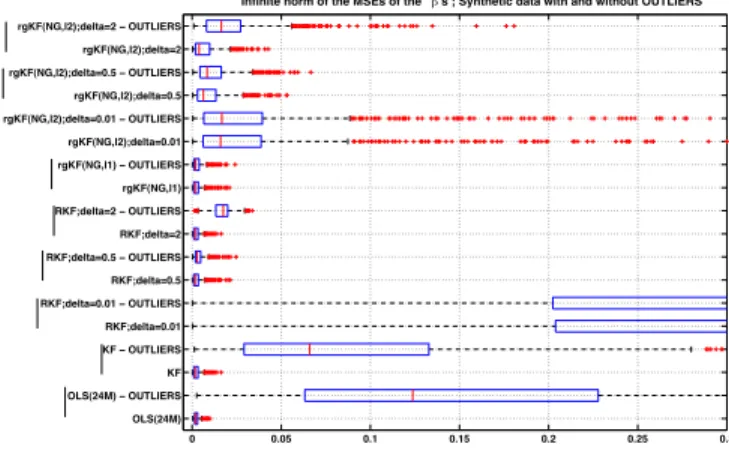
This procedure is run 1000 times in order to evaluate the MSEs of the parameter estimations for the different algorithms. The MSEs distributions are displayed on Fig. 2 as boxplots. For each simulation, we keep the maximum of the ’s MSEs. As a benchmark method, we have compared the results to those obtained by using a 24-long rolling window ordinary least squares (OLS) regression to estimate the constant parameters. OLS is known to deliver the optimum solution in such a setting (regression with constant coefficient) and acts therefore as the lower bound for optimality. As expected, OLS gives the lowest estimation errors when no outlier is present, followed by KF in the same situation. When outliers are added, then rgKF(NG,l1₎ gives a similar performance as in the no outlier case and tends to deliver the same performance as a KF with no outlier. RKF and rgKF(NG,l2_{) performance depends on the choice of .} Setting = 0.01 for RKF yields the entire sets of observations to be considered as outliers.

C. Hedge funds returns

This section is devoted to applying rgKF(NG, l1_{) on real} hedge funds data to detect the potential occurrence of outliers. We conduct the analysis on returns of Global Macro hedge funds. Managers of such funds take directional positions in currencies, debt, equities, or commodities and may also elect to take relative positions combining long positions paired off against short positions. Hedge funds data comes from the

0 0.05 0.1 0.15 0.2 0.25 0.3 OLS(24M) OLS(24M) − OUTLIERS KF KF − OUTLIERS RKF;delta=0.01 RKF;delta=0.01 − OUTLIERS RKF;delta=0.5 RKF;delta=0.5 − OUTLIERS RKF;delta=2 RKF;delta=2 − OUTLIERS rgKF(NG,l1) rgKF(NG,l1) − OUTLIERS rgKF(NG,l2);delta=0.01 rgKF(NG,l2);delta=0.01 − OUTLIERS rgKF(NG,l2);delta=0.5 rgKF(NG,l2);delta=0.5 − OUTLIERS rgKF(NG,l2);delta=2 rgKF(NG,l2);delta=2 − OUTLIERS

Infinite norm of the MSEs of the ’s ; Synthetic data with and without OUTLIERS

Fig. 2. Distribution of the 1000 maxima of the ’s MSEs computed for

each of the 1000 synthetic time series of returns of size 150, with or without additional outliers.

hedge fund research (HFR) database [14]. The returns are end-of-month returns, available from January 1998 to June 2010 (i.e. for 150 months).

We choose the eight risk factors of Fung & Hsieh (F&H) [15], selected and constructed by the authors [13] to explain trend-follower hedge funds. These factors are now widely used in the literature of hedge funds analysis. They are quoted on a monthly basis and stored in ft at each end-of-month t. Fig. 3 illustrates the capability of the rgKG(NG,l1_{) to detect,} estimate and filter some points in the observed returns time series which might be considered as hedge fund’s specific events, outliers, irregularities or illiquidity issues. As it can be seen on the top graph of Fig. 3, when an outlier occurs, then the resulting KF estimations of suddenly jump to four or five times their previous values whereas no special event occurs in the market.

Jan00 Jan01 Jan02 Jan03 Jan04 Jan05 Jan06 Jan07 Jan08 Jan09 Jan10

−0.1 0 0.1 0.2 0.3 HF returns estimated spikes 0

0.5 OSV Currency Fund: KF exposures

−0.5 0 0 0.2 0.4 0.6 0.8

OSV Currency Fund: rgKF(NG,l1_{) exposures}

−0.5 0

PTFSBD PTFSFX PTFSCOM SP500 EquitySizeSpread bond10y creditSpread MXEF

Fig. 3. Outliers detection and estimation for the OSV Currency Fund returns. Impact of outliers on the fund’s exposures can be observed on the top graph of the figure: KF does not filter the rgKF(NG,l1_{) estimated spikes and gives}

misled estimations of the market risks.

VI. CONCLUSION

This article has presented a new family of algorithms named rgKFs for regularized KFs which have been derived to Detect

and Estimate exogenous outliers that might occur in the observations equation of a standard Kalman Filter. Inspired from the Robust Kalman Filter (RKF) of [8] which makes use of a l1_{-regularization step, we introduce a simple but} efficient detection step in the recursive equations of the RKF. This solution is one way to solve the problem of adapting the value of the l1_{-regularization parameter: when an outlier} is detected in the innovation term of the KF, then the value of the regularization parameter is set to a value that will let the l1_{-based optimization problem estimate the amplitude of} the spike. We have also tested a l2_{-based regularization term} for which the solution is known in a closed form. The results obtained on synthetic data show that the best performance are achieved by the rgKF(NG,l1_{) that handles the choice of the} regularization parameter. In the context of analyzing hedge funds returns the rgKF(NG,l1_{) could help risk managers to} dynamically and accurately estimate the exposures of hedge funds for which they do not have any other information than the observed returns. Interpreting outliers as illiquidity issues, our algorithms would therefore be very useful to classify funds according to their ”illiquidity quality” and to make accurate decisions from a regulation point of view.

REFERENCES

[1] A. J. Fox, “Outliers in time series,” Journal of the Royal Statistical Society, Series B, vol. 34, pp. 350–363, 1972.

[2] P. Ruckdeschel, “Optimally robust kalman filtering,” Berichte des Fraunhofer ITWM 185, Fraunhofer, ITWM, May 2010.

[3] R. A. Maronna, R. D. Martin, and V. J. Yohai, Robust Statistics, Theory and Methods, John Wiley & Sons, 2006.

[4] R. Tibshirani, “Regression shrinkage and selection via the LASSO,” Journal of the Royal Statistical Society, vol. 58, no. Series B, pp. 267– 288, 1996.

[5] R. Jagannathan and T. Ma, “Risk reduction in large portfolios: why imposing the wrong constraints helps,” Journal of Finance, vol. 58, no. 4, pp. 1651–1684, 2003.

[6] J. Brodie, I. Daubechies, C. De Mol, D. Giannone, and I. Loris, “Sparse and stable markowitz portfolios,” September 2008, European Central Bank Working Paper No 936.

[7] V. DeMiguel, L. Garlappi, F. J. Nogales, and R. Uppal, “A generalized approach to portfolio optimization: improving performance by constrain-ing portfolio norms,” Management Science, vol. 55, no. 5, pp. 798–812, May 2009.

[8] J. Mattingley and S. Boyd, “Real-time convex optimization in signal processing,” IEEE Signal Processing Magazine, vol. 27, no. 3, pp. 50– 61, May 2010.

[9] M. R. Osborne, B. Presnell, and B. A. Turlach, “On the LASSO and its dual,” Journal of Computational and Graphical Statistics, vol. 9, no. 2, pp. 319–337, June 2000.

[10] M. Schmidt, “Least squares optimization with L1_{-norm regularization,”}

Project Report CS542B, UBC, University of Alberta, Canada, December 2005.

[11] E. Jay, P. Duvaut, S. Darolles, and A. Chr´etien, “Multi-factor models : examining the potential of signal processing techniques,” IEEE Signal Processing Magazine, vol. 28, no. 5, September 2011.

[12] D. A. Hsieh, “Data library webpage: Hedge fund risk factors,”

http://faculty.fuqua.duke.edu/%7Edah7/HFRFData.htm.

[13] W. Fung and D. Hsieh, “The risk in hedge fund strategies, theory and evidence from trend followers,” Review of Financial Studies, vol. 14, no. 2, pp. 313–341, 2001.

[14] Hedge Fund Research, “HFR databases,”

http://www.hedgefundresearch.com/.

[15] D. A. Hsieh, “Data library webpage: Hedge fund risk factors,” http: //faculty.fuqua.duke.edu/\%7Edah7/HFRFData.htm.