On the complexity of the exact weighted
independent set problem
1.1. Introduction
Suppose we have a well-solved optimization problem, such as minimum spanning tree, maximum cut in planar graphs, minimum weight perfect matching, or maxi-mum weight independent set in a bipartite graph. How hard is it to determine whether there exists a solution with a given weight ? Papadimitriou and Yannakakis showed in [PAPADIMITRIOU 82] that these so-called exact versions of the above optimiza-tion problems are NP-complete when the weights are encoded in binary. The quesoptimiza-tion is then, what happens if the weights are « small », i.e., encoded in unary ? Contrary to the binary case, the answer to this question depends on the problem.
– The exact spanning tree problem, and more generally, the exact arborescence problem are solvable in pseudo-polynomial time [BARAHONA 87].
– The exact cut problem is solvable in pseudo-polynomial time for planar and toroidal graphs [BARAHONA 87].
– The exact perfect matching problem is solvable in pseudo-polynomial time for planar graphs [BARAHONA 87], and more generally, for graphs that have a Pfaffian orientation1(provided one is given). We recall that a matching of a graph G = (V, E)
is a set E0 of pairwise non-adjacent edges of G. If |E0| = |V |/2, then E0 is said to
be a perfect matching of G. Karzanov [KARZANOV 87] gives a polynomial-time Chapitre rédigé par Martin MILANI ˇCet Jérôme MONNOT.
1. Bipartite graphs with a Pfaffian orientation have been characterized in [THOMAS 06], where a polynomial-time recognition algorithm is also presented.
algorithm for the special case of the exact perfect matching problem, when the graph is either complete or complete bipartite, and the weights are restricted to 0 and 1. Papadimitriou and Yannakakis show in [PAPADIMITRIOU 82] that the problem for general (or bipartite) graphs with weights encoded in unary is polynomially reducible to the one with 0-1 weights. Mulmuley, Vazirani and Vazirani [MULMULEY 87] show that the exact perfect matching problem has a randomized pseudo-polynomial-time algorithm.
The exact perfect matching problem is of great practical importance. It has
applica-tions in such diverse areas as bus-driver scheduling, statistical mechanics (see [LECLERC 86]), DNA sequencing [BŁA ˙ZEWICZ 06], and robust assignment problems [DE˘INEKO 06].
The problem consists in determining whether a given edge-weighted graph contains a perfect matching of a given weight. Despite polynomial results for special cases, the deterministic complexity of the exact perfect matching problem remains unset-tled for general graphs, and even for bipartite graphs. Papadimitriou and Yannakakis conjectured that the problem is NP-complete [PAPADIMITRIOU 82].
This open problem motivates us to introduce and study the exact weighted inde-pendent set problem and a restricted version of it, both closely related to the exact perfect matching problem.
An independent set (sometimes called stable set) in a graph is a set of pairwise non-adjacent vertices. The weighted independent set problem (WIS) asks for an in-dependent set of maximum weight in a given weighted graph (G, w). If all weights are the same, we speak about the independent set problem (IS). The optimal values of these problems are denoted by αw(G) and α(G), respectively.
The exact weighted independent set problem (EWIS) consists of determining whe-ther a given weighted graph (G, w) with G = (V, E) and w : V → Z contains an independent set whose total weight (i.e., the sum of the weights of its members) equals a given integer b. Formally, the solution to the EWIS problem, given (G, w, b), is yes if and only if there is an independent set I of G with w(I) = b. The restriction where we require the independent set to be of a maximum independent set of the graph will be called the exact weighted maximum independent set problem and denoted by EWISα.
Thus, EWISα(G, w, b) asks about the existence of an independent set I of G with
|I| = α(G) and w(I) = b.
The connection between the exact perfect matching problem and the exact weigh-ted independent set problem is best understood through line graphs. The line graph L(G) of a graph G = (V, E) is the graph whose vertex set is E, and whose two ver-tices are adjacent if and only if they share a common vertex as edges of G. Clearly, there is a one-to-one correspondence between the matchings of a graph and the in-dependent sets of its line graph. The exact matching problem, that is, the problem of determining whether a given edge-weighted graph contains a matching of a given
weight, is then precisely the exact weighted independent set problem, restricted to the class of line graphs. Similarly, under the (polynomially verifiable) assumption that the input graph has a perfect matching, the exact perfect matching problem is precisely the exact weighted maximum independent set problem, restricted to the class of the line graphs of graphs with a perfect matching.
In this chapter, we focus on the problem of determining the complexities of the EWIS and EWISαproblems for particular graph classes. On the one hand, we present
the first nontrivial strong NP-completeness result for these problems. On the other hand, we distinguish several classes of graphs where the problems can be solved in pseudo-polynomial time.
More specifically, we can summarize the main results of this chapter in the spirit of the above list of complexity results on exact problems :
– The exact weighted independent set and the exact weighted maximum inde-pendent set problems are strongly NP-complete for cubic bipartite graphs.2
– The exact weighted independent set and the exact weighted maximum inde-pendent set problems are solvable in pseudo-polynomial time in each of the following graph classes :
- mK2-free graphs,
- interval graphs, and their generalizations k-thin graphs, - circle graphs,
- chordal graphs, - AT-free graphs,
- (claw , net)-free graphs, - distance-hereditary graphs, - graphs of bounded treewidth, - graphs of bounded clique-width,
- certain subclasses of P5-free and fork-free graphs.
The results for subclasses of P5-free and fork-free graphs are derived by means
of modular decomposition. The application of modular decomposition to the EWIS problem is described in Section 1.4.2 and may be of independent interest.
In view of the relation between the exact perfect matching problem and the exact weighted maximum independent set problem, each of the above polynomial results also gives a polynomial result for the exact perfect matching problem. Whenever the EWISαproblem is (pseudo-) polynomially solvable for a class of graphs G, the exact 2. We also strengthen this result considerably, however we postpone the detailed formulation until Section 1.3.2.
perfect matching problem is (pseudo-) polynomially solvable for graphs in the set {G : L(G) ∈ G}. For example,
– The exact perfect matching problem is solvable in pseudo-polynomial time for graphs of bounded treewidth.
Notation and organization. All graphs considered are finite, simple and undirected. Unless otherwise stated, n and m will denote the number of vertices and edges, res-pectively, of the graph considered. As usual, Pnand Cndenote the chordless path and
the chordless cycle on n vertices. For a graph G, we will denote by V (G) and E(G) the vertex-set and the edge-set of G, respectively. Individual edges will be denoted by square brackets : an edge with endpoints u and v will be denoted by [u, v]. For a vertex x in a graph G, we denote by NG(x) the neighborhood of x in G, i.e., the
set of vertices adjacent to x, and by NG[x] the closed neighborhood of x, i.e., the
set NG(x) ∪ {x}. We will write N (x) and N [x] instead of NG(x) and NG[x] if no
confusion can arise.
We say that a graph H is an induced subgraph of G if H can be obtained from G by deletion of some (possibly none) vertices ; the subgraph of G induced by U ⊆ V (G) is the graph obtained from G by deleting the vertices from V (G)\U and it will be deno-ted by G[U ]. For a graph G, we denote by co-G (also G) the edge-complement of G. By Knwe denote the complete graph on n vertices, and by Ks,tthe complete bipartite
graph with parts of size s and t. By component we will always mean a connected com-ponent. For graph-theoretical terms not defined here, the reader is referred to Berge’s book [BERGE 73]. For a subset of vertices V0 ⊆ V , we let w(V0) =P
v∈V0w(v).
For a positive integer k, we write [k] for the set {1, . . . , k}.
The triple (G, w, b) will always represent an instance of the EWIS (or EWISα)
problem, i.e., G = (V, E) is a graph, w : V → Z are vertex weights, and b ∈ Z is the target weight. If H is an induced subgraph of G, we will also consider triples of the form (H, w, b) as instances of EWIS, with the weights w representing the restriction of w to V (H). We will denote by EWIS(G, w, b) the solution to the instance (G, w, b) of the EWIS problem, that is, EWIS(G, w, b) is yes if there is an independent set I in G with w(I) = b, and no otherwise. Similarly, EWISα(G, w, b) is yes if there is a
maximum independent set I in G with w(I) = b, and no otherwise.
The chapter is organized as follows. In Section 1.2, we continue the introductory discussion and present some polynomial preprocessing steps that simplify the input and which we will later on assume performed. We also discuss some relations between the complexities of the problems WIS, EWIS and EWISα. Section 1.3 is devoted to
the strong NP-completeness results. In Section 1.4, pseudo-polynomial time solutions to the exact weighted independent set problem are presented. We conclude the chapter with a short discussion in Section 1.5 that places the class of line graphs of bipartite graphs between two graph classes with known complexities of the EWIS problem.
1.2. Preliminary observations
The exact weighted independent set problem is (weakly) NP-complete for any class of graphs containing the edgeless graphs {Kn : n ≥ 0}. There is a direct
equi-valence between the exact weighted independent set problem on {Kn : n ≥ 0} and
the subset sum problem, which is known to be NP-complete (see [GAREY 79]). The subset sum problem is the following : given n integers a1, . . . , an and a bound b,
determine whether there is a subset J ⊆ [n] such thatPj∈Jaj= b.
Therefore, for a given class of graphs G, the question of interest is whether the EWIS problem is strongly NP-complete for graphs in G, or is it solvable in pseudo-polynomial time.
First, let us observe that in any class of graphs G, we may restrict our attention to instances with positive weights only.
REMARQUE 1.– The EWIS problem with arbitrary integer weights is polynomially
equivalent to the EWIS problem, restricted to instances (G, w, b) such that b ≤ w(V (G)) and 1 ≤ w(v) ≤ b, for all v ∈ V . The same equivalence holds true for the EWISα
problem.
PREUVE.– Solving the EWIS problem for any particular instance reduces to solving
n problems EWISk, in which the independent sets are restricted to be of size k, for
all k ∈ [n] (unless b = 0, in which case the solution is trivial, as the empty set is an independent set of weight 0). The weights in EWISk can be assumed to be positive :
otherwise, we can add a suitably large constant N to each vertex weight and replace b by b + kN to get an equivalent EWISk problem with positive weights only. Finally,
applying the same transformation again with N = w(V ) + 1 reduces the problem EWISkto a single EWIS problem with positive weights. Repeating this for all values
of k ∈ [n], the result follows.
Finally, if all vertex weights are positive, we can delete from the graph all vertices whose weight exceeds b, as they will never appear in a solution. Furthermore, the solution is clearly no if b > w(V ).
The same assumption on vertex weights as for the EWIS problem can also be made for the instances (G, w, b) of its restricted counterpart EWISα. Again, if some
of the weights are negative, we can modify the weights and the target value as we did above for EWISk. Now we only do it for k = α(G). Note that we can compute α(G)
as that only p ∈ [n] such that the value of EWISα(G, 1, p) is yes, where 1 denotes the
unit vertex weights.
We now discuss some relations between the complexities of the problems WIS, EWIS and EWISα, when restricted to particular graph classes.
LEMME1.1.– Let G be a class of graphs. The following statements are true.
(i) If the EWISαproblem is solvable in pseudo-polynomial time for graphs in G, then
the WIS problem is solvable in pseudo-polynomial time for graphs in G.
(ii) If the EWIS problem is solvable in pseudo-polynomial time for graphs in G, then the EWISαproblem is solvable in pseudo-polynomial time for graphs in G.
(iii) Let G0= {G0: G ∈ G} where G0= (V0, E0) is the graph, obtained from a graph
G = (V, E) ∈ G, by adding pendant vertices, as follows : V0 = V ∪ {v0 : v ∈ V },
E0 = E ∪ {[v, v0] : v ∈ V }. If the EWIS
αproblem is solvable in pseudo-polynomial
time for graphs in G0, then the EWIS problem is solvable in pseudo-polynomial time
for graphs in G.
PREUVE.– (i) Let (G, w, k) be an instance of the decision version of the weighted
in-dependent set problem. As we can assume positive weights, G contains an inin-dependent set of total weight at least k if and only if G contains a maximum independent set of total weight at least k. By testing values for b from w(V ) down to k and using an algorithm for the EWISαproblem on the instance (G, w, b), we can decide whether
G contains a maximum independent set of total weight at least k.
(ii) Let (G, w, b) be an instance of the EWISα problem. It is easy to see that the
following algorithm solves EWISα.
Step 1. Compute α(G), which is equal to the maximum k ∈ [n] such that the value of EWIS(G, 1, k) is yes, where 1 denotes the unit vertex weights.
Step 2. Let N = w(V ) + 1. For every vertex v ∈ V (G), let w0(v) = w(v) + N . Let
b0= b + α(G)N . Then it is easy to verify that EWIS
α(G, w, b) = EWIS(G, w0, b0).
(iii) Let (G, w, b) with G = (V, E) ∈ G be an instance of the exact weighted inde-pendent set problem. Let G0 be the graph, defined as in the lemma. Let n = |V (G)|
and let w0(v) = (n + 1)w(v) for all v ∈ V and w0(v) = 1 for v ∈ V0. Then, it
is easy to verify that the value of EWIS(G, w, b) is yes if and only if the value of EWISα(G0, w0, b0) is yes for some b0 ∈ {(n + 1)b, . . . , (n + 1)b + n − 1}.
The problem EWIS is clearly in NP, and so is EWISα for any class of graphs
G where IS is polynomially solvable. Therefore, Lemme 1.1 implies the following result.
COROLLAIRE1.1.– Let G be a class of graphs. The following statements are true.
(i) If the WIS problem is strongly NP-complete for graphs in G, then the EWISα
pro-blem is strongly NP-hard for graphs in G. If, in addition, the IS propro-blem is polynomial for graphs in G, then the EWISαproblem is strongly NP-complete for graphs in G.
(ii) If the EWISαproblem is strongly NP-hard for graphs in G, then the EWIS
pro-blem is strongly NP-complete for graphs in G.
graphs in G, then the EWISα problem is strongly NP-hard for graphs in G0. If, in
addition, the IS problem is polynomial for graphs in G0, then the EWIS
αproblem is
strongly NP-complete for graphs in G0.
Thus, we are mainly interested in determining the complexity (strong NP-complete or pseudo-polynomial results) of the exact weighted independent set problem in those classes of graphs where the weighted independent set problem is solvable in pseudo-polynomial time. Moreover, combining parts (ii) and (iii) of the lemma shows that when G ∈ {forests, bipartite graphs, chordal graphs}, the problems EWIS and EWISα
are equivalent (in the sense that, when restricted to the graphs in G, they are either both solvable in pseudo-polynomial time, or they are both strongly NP-complete). Recall that a graph G is a forest if it is acyclic, bipartite if any cycle of G has even length, and chordal if any cycle of G with size at least 4 has a chord (i.e., an edge connecting two nonconsecutive vertices of the cycle).
We conclude this subsection by showing that a similar equivalence remains valid for the class of line graphs. More precisely, if L, L(Bip), L(K2n) and L(Kn,n) denote
the classes of line graphs, line graphs of bipartite graphs, line graphs of complete graphs with an even number of vertices, and line graphs of complete balanced bipartite graphs, respectively, we have the following result.
LEMME1.2.– The EWIS problem is strongly NP-complete for graphs in L (resp.,
L(Bip)) if and only if the EWISα problem is strongly NP-complete for graphs in
L(K2n) (resp., L(Kn,n)).
PREUVE.– The backward implication is given by part (ii) of Lemme 1.1. The
for-ward implication follows from a reduction of the exact matching problem to the exact perfect matching problem which we show now. Given an instance G = (V, E) with edge weights w and a target b for the exact matching problem, construct an instance (Kn0, w0, b0) for the exact perfect matching problem as follows. If n = |V | is odd, we
add a new vertex and we complete the graph G. For an edge e of G, let w0(e) = N w(e)
where N = w(E) + 1, for an edge e /∈ E let w0(e) = 1. The transformation is clearly
polynomial, and G has a matching of weight b if and only if Kn0 has a perfect
mat-ching of weight N b + k for some value of k ∈ {0, . . . , n − 1}. Also, it is easy to see that in the case of bipartite graphs G = (L, R; E) with |L| ≤ |R|, we can add |R \ L| vertices to L to balance the bipartition.
1.3. Hardness results
The weighted independent set problem is solvable in polynomial time for bipartite graphs by network flow techniques. However, as we show in this section, the exact version of the problem is strongly NP-complete even for cubic bipartite graphs.
1.3.1. Bipartite graphs
A bipartite graph is a graph G = (V, E) whose vertex set admits a partition V = L ∪ R into the left set L and the right set R such that any edge of G connects a vertex of L to a vertex of R. In general, a bipartite graph may admit several such partitions. Since we only consider connected bipartite graphs (which have a unique such partition, up to switching the parts), we will also write G = (L, R; E).
The strong NP-completeness of the EWIS problem in bipartite graphs follows from a straightforward reduction from the balanced biclique problem which is known to be NP-complete [GAREY 79]. The balanced biclique problem consists in deter-mining whether, given a bipartite graph G = (L, R; E) and an integer k, there exist subsets L0 ⊆ L and R0 ⊆ R with |L0| = |R0| = k such that the subgraph
in-duced by L0∪ R0 is a complete bipartite subgraph (also called biclique of size k).
In [DAWANDE 01], a variation of this latter problem is introduced where we must have |L0| = a and |R0| = b (called the biclique problem). From an instance G and
k of balanced biclique, we introduce weight 1 on each vertex of L, weight B = max{|L|, |R|} + 1 on each vertex of R, and we set b = k + Bk. It is clear that there exist an independent set in (L, R; (L × R) \ E) with weight b if and only if there exists a balanced biclique in (L, R; E) of size k.
We now strengthen this result by proving that the EWISαproblem is strongly
NP-complete for cubic bipartite graphs. By contrast, for graphs of maximum degree 2, EWIS and EWISα are pseudo-polynomially solvable problems. Every connected
graph in this class is either a cycle or a path, and the treewidth of such graphs is at most 2.3By Corollaire 1.3 and Théorème 1.14 from Section 1.4, the problem is
solvable in pseudo-polynomial time in this class.
THÉORÈME1.1.– The EWISαproblem is strongly NP-complete in cubic bipartite
graphs.
PREUVE.– The problem is clearly in NP, as the IS problem is solvable in
polyno-mial time for bipartite graphs. The hardness reduction is made from the decision version of the clique problem in regular graphs which is known to be NP-complete, see [GAREY 79]. A clique V∗ is a subset of vertices of G such that the subgraph
induced by V∗ is complete. Let (G, k) be an input to the clique problem, where
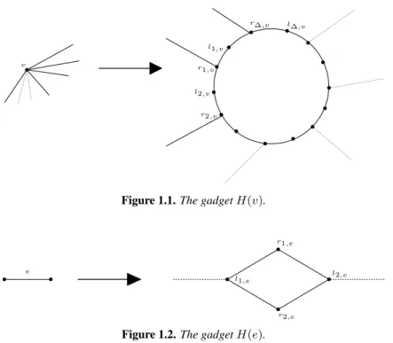
G = (V, E) is a ∆-regular graph on n vertices and let k be an integer. Without loss of generality, assume that 0 < k < ∆ < n − 1, since otherwise the problem is easy. We build the instance I = (G0, w) of the EWIS
αproblem where G0 = (L, R; E0) is
a bipartite graph as follows :
l∆,v v r∆,v l1,v r1,v l2,v r2,v
Figure 1.1. The gadget H(v).
l2,e e
l1,e r1,e
r2,e
Figure 1.2. The gadget H(e).
• For each vertex v ∈ V , we construct a gadget H(v) which is a cycle of length 2∆. Thus, it is a bipartite graph where the left set is Lv= {l1,v, . . . , l∆,v} and the right
set is Rv= {r1,v, . . . , r∆,v}. The weights are w(li,v) = 1 and w(ri,v) = n∆(2+n∆2 )
for i ∈ [∆]. The gadget H(v) is illustrated in Figure 1.1.
• For each edge e ∈ E, we construct a gadget H(e) which is a cycle of length 4. Thus, it is a bipartite graph where the left set is Le= {l1,e, l2,e} and the right set is
Re= {r1,e, r2,e}. The weights are w(li,e) = (n∆)2 and w(ri,e) = (n∆)
2
2 (2+n∆2 ) for
i = 1, 2. The gadget H(e) is illustrated in Figure 1.2.
• We interconnect these gadgets by iteratively applying the following procedure. For each edge e = [u, v] ∈ E, we add two edges [ri,u, l1,e] and [li,u, r1,e] where li,u
is a neighbor of ri,uin H(u) between gadgets H(u), H(e) and two edges [rj,v, l2,e]
and [lj,v, r2,e] where lj,vis a neighbor of rj,v in H(v) between gadgets H(v), H(e)
such that the vertices ri,u, li,u, rj,vand lj,vhave degree 3.
It is clear that G0is bipartite and the weights are polynomially bounded. Moreover,
We claim that there exist a clique V∗of G with size at least k if and only if the
value of EWISα(G0, w, b) is yes, where
b = k∆ + n∆k(k − 1) 2 + n∆( 2 + n∆ 2 ) µ (n − k)∆ + (n∆ 2 − k(k − 1) 2 )n∆ ¶ .
Let I be a maximum independent set of G0 with w(I) = b. Since G0 is cubic
and bipartite, G0has a perfect matching (for instance, take a perfect matching in each
gadget H(v) and H(e)), and we conclude that α(G) = |I| = |R| = |L|. This implies in particular that for any vertex v ∈ V , either Lv or Rv is a subset of I. Moreover,
the same property holds for any e ∈ E (i.e., either Le or Reis a subset of I). By
construction of the weights, the quantity k∆ of b must come from vertices li,v, ri,vor
li,e. Since k < n, this quantity cannot come from ri,v. Moreover, since li,e∈ I if and
only if Le⊆ I, the contribution of Lein I is n∆. In this case, the contribution of k∆
must come from li,v. Thus, we obtain :
|I ∩ LV| = k∆ , |I ∩ RV| = (n − k)∆. [1.1]
where LV = ∪v∈VLvand RV = ∪v∈VRv. Thus, using (1.1) we must obtain :
w (I ∩ (LE∪ RE)) = n∆k(k − 1) 2 +n∆( 2 + n∆ 2 )( n∆ 2 − k(k − 1) 2 )n∆.[1.2] where LE = ∪e∈ELeand RE = ∪e∈ERe. Now, we prove that there are exactly
k(k−1
2 ) gadgets H(e) with Le ⊆ I. Assume the converse ; then, |I ∩ LE| = k(k −
1) − 2p and |I ∩ RE| = n∆ − k(k − 1) + 2p for some p 6= 0 (p can be negative).
Combining these equalities with equality (1.2), we deduce that p = 0, contradiction. Thus, if we set V∗ = {v ∈ V : L
v ⊆ I}, we deduce from above that |V∗| = k
and we will have necessarily that V∗is a clique of G.
Conversely, let V0 be a clique of G with |V0| ≥ k and consider a subclique V∗⊆
V0 of size exactly k. We set S = S
L∪ SR with SL = ∪v∈V∗Lv∪e∈E(V∗)Leand
SR = ∪v∈V \V∗Rv∪e∈E\E(V∗)Re. One can easily verify that w(I) = b and that I
is a maximum independent set of G0. Indeed, let us assume the converse ; thus, there
exist ri,v ∈ I (and thus Rv ⊆ I), lj,e ∈ I (with j = 1, 2) and [ri,v, lj,e] ∈ E0. By
construction of I, we deduce that e = [u, v] ∈ E(V∗) and then L
v⊆ I, contradiction.
As corollary of Théorème 1.1, we can derive that the biclique problem remains NP-complete when the minimum degree of G = (L, R; E) is n − 3 where |L| = |R| = n. In this case, we replace any gadget H(e) of Théorème 1.1 by a cycle of length 2n∆ and we delete edges [li,u, r1,e] and [lj,v, r2,e].
We also remark that Théorème 1.1 implies the strong NP-completeness of the EWISα problem for perfect graphs, a well-known class where the weighted
inde-pendent set problem is solvable in polynomial time [GRÖTSCHEL 84].
1.3.2. A more general hardness result
Let us now strengthen the main result of the previous subsection. To this end, we first introduce some notations. Let F be a set of graphs. We denote the class of graphs containing no induced subgraphs from the set F by Free(F). Any graph in Free(F) will be called F-free. Our hardness results will be expressed in terms of a parameter related to the set of forbidden induced subgraphs F.
Let Ciand Hidenote the cycle of length i and the graph in Figure 1.3, respectively.
c c c ` ` c ` c c c c c 1 2 i Figure 1.3. Graph Hi
We associate to every graph G a parameter κ(G), which is the minimum value of i ≥ 1 such that G contains an induced copy of either Cior Hi. If G is an acyclic graph
with no induced graphs of the form Hi, we let κ(G) = ∞. For a (possibly infinite)
nonempty set of graphs F, we define
κ(F) = sup { κ(G) : G ∈ F } .
Finally, for a set of graphs X, let X3denote the set of graphs of degree at most 3 in X.
With these definitions in mind, we can use the strong NP-completeness of the EWISα problem for bipartite graphs of degree at most 3 (which is an immediate
corollary of Théorème 1.1), and the reduction typically used for the IS problem (see e.g. [MURPHY 92, POLJAK 74]), to derive the following hardness result.
THÉORÈME1.2.– Let G be the class of F-free bipartite graphs of maximum degree at most 3. If κ(F3) < ∞, then the EWISα problem is strongly NP-complete in the
class G3.
PREUVE.– The problem is clearly in NP. We show completeness in two steps. First,
for k ≥ 3, let Skbe the class of all bipartite (C3, . . . , Ck, H1, . . . , Hk)-free graphs of
vertex degree at most 3, and let us show that for any fixed k, the problem is strongly NP-complete for graphs in Sk. Let (G, w, b) be an instance of the EWISαproblem
where G is a bipartite graph of maximum degree at most 3.
We can transform the graph G in polynomial time to a weighted graph G0, as
follows. Let k0 = dk
2e. We replace each edge e of G by a path P (e) on 2k0 + 2
vertices. Let N = w(V ) + 1. We set the weights w0 of the endpoints of P (e) equal
to the weights of the corresponding endpoints of e, while each internal vertex of P (e) gets weight N . It is easy to verify that G0belongs to S
k.
We claim that the value of EWISα(G, w, b) is yes if and only if the value of
EWISα(G0, w0, b + mk0N ) is yes, where m = |E(G)|.
One direction is immediate, as each maximum independent set of G can be ex-tended to a maximum independent set of G0, by simply adding k0internal vertices of
each newly added path. Doing so, the weight increases by mk0N .
Suppose now that the value of EWISα(G0, w0, b + mk0N ) is yes. Let I0 be a
maximum independent set of G0 of weight b + mk0N . Since I0 is independent, it
can contain at most k0internal vertices of each newly added path. Therefore, for each
e ∈ E(G), the set I0 must contain exactly k0internal vertices of P (e) – otherwise its
weight would be at most w(V ) + (mk0− 1)N , contradicting our choice of N .
Let I denote the set, obtained from I0 by deleting the internal vertices of newly
added paths. Then, I is an independent set of G. Indeed, if e = [u, v] ∈ E(G) for some u, v ∈ I, then I0would contain at most k0− 1 internal vertices of P (e), contradicting
the above observation. Also, it is easy to see that I is a maximum independent set of G. Finally, as the weight of I is exactly b, we conclude that the value of EWISα(G, w, b)
is yes.
This shows that the EWISαproblem is strongly NP-complete in the class Sk. To
prove strong NP-completeness of the problem in the class G3, we now show that the
class G3 contains all graphs in Sk, for k := max{3, κ(F)}. Let G be a graph from
Sk. Assume that G does not belong to G3. Then G contains a graph A ∈ F3 as an
induced subgraph. From the choice of G we know that A belongs to Sk, but then
k < κ(A) ≤ κ(F3) ≤ k, a contradiction. Therefore, G ∈ G3 and the theorem is
1.4. Polynomial results
In this section, we present pseudo-polynomial solutions to the exact weighted in-dependent set problem, when the input graphs are restricted to particular classes.4The
algorithms resemble those for the WIS problem in respective graph classes, and are based either on a dynamic programming approach (Section 1.4.1), or on the modular decomposition (Section 1.4.2).
First, we observe that when developing polynomial-time solutions to the EWIS problem, we may restrict our attention to connected graphs.
LEMME1.3.– Let (G, w, b) be an instance of the EWIS problem, and let C1, . . . , Cr
be the connected components of G. Suppose that for each i ∈ [r], the set of solutions (EWIS(Ci, w, k) : k ∈ [b]) for Ciis given. Then, we can compute the set of solutions
(EWIS(G, w, k) : k ∈ [b]) for G in time O(rb2).
In order to show Lemme 1.3, we consider the following generalization of the subset sum problem.
GENERALIZEDSUBSETSUM(GSS)
Instance : Nonempty sets of positive integers A1, . . . , Anand a positive integer b.
Question : Is there a nonempty subset J of [n] and a mapping a : J → ∪j∈JAjsuch
that a(j) ∈ Aj for all j ∈ J, and
P
j∈Ja(j) = b ?
By generalizing the dynamic programming solution to the subset sum problem, it is easy to show the following.
LEMME 1.4.– Generalized subset sum can be solved in time O(nb2) by dynamic
programming.
In fact, in the stated time, not only we can verify if there is a J ⊆ [n] and a mapping a as above such thatPj∈Ja(j) = b for the given b, but we can answer this question for all values b0∈ [b].
PREUVE.– Let B denote the set of all values b0 ∈ [b] such that there a nonempty
subset S of [n] and a mapping a : S → ∪i∈SAisuch that a(i) ∈ Aifor all i ∈ S, and
P
i∈Sa(i) = b0.
Let us show by induction on n that we can generate the set B in time O(nb2). The
statement is trivial for n = 1.
Suppose now that n > 1. Let I = (A1, . . . , An; b) be an instance of the GSS
problem. Let B0 be the inductively constructed set of all possible values of b0 ∈ [b]
such that the solution to the GSS problem on the instance (A1, . . . , An−1; b0) is yes.
By induction, the set B0was constructed in time O((n − 1)b2).
Let β ∈ [b]. Then, β will belong to B, i.e., the solution to the GSS problem, given (A1, . . . , An; β), will be yes, if and only if either β ∈ B0, or we can write β as
β = b0+ a
nfor some b0∈ B0and an∈ An. In other words, B = B0∪ B00, where B00
denotes the set of all such sums : B00= {b0+ a
n : b0 ∈ B0, an∈ An, b0+ an≤ b}.
The set B00can be constructed in time O(b2). Adding this time complexity to the
time O((n − 1)b2) needed to construct B0 proves the above statement and hence the
lemma.
Lemme 1.3 now follows immediately.
PREUVE.– [Lemme 1.3] It is enough to observe that for every k ∈ [b], the value of EWIS(G, w, k) is yes if and only if the solution to the GSS problem on the ins-tance (A1, . . . , Ar; k) is yes, where Aidenotes the set of all values k0∈ [b] such that
EWIS(Ci, w, k0) is yes.
1.4.1. Dynamic programming solutions
We can summarize the results of this subsection in the following theorem. THÉORÈME1.3.– The exact weighted independent set and the exact weighted maxi-mum independent set problems admit pseudo-polynomial-time solutions in each of the following graph classes : mK2-free graphs, interval graphs and their generalizations
k-thin graphs, circle graphs, chordal graphs, AT-free graphs, (claw , net)-free graphs, distance-hereditary graphs, graphs of treewidth at most k, and graphs of clique-width at most k.
The rest of this subsection is devoted to proving this result. By part (ii) of Lemme 1.1, it suffices to develop pseudo-polynomial solutions for the EWIS problem. Most of the algorithms resemble those for the WIS problem and exploit the special structure of graphs in the classes.
1.4.1.1. mK2-free graphs
Our first example deals with graphs with no large induced matchings.
Recall that K2denotes the graph consisting of two adjacent vertices. The disjoint
union of m copies of K2 is denoted by mK2. Thus, graphs whose largest induced
THÉORÈME1.4.– For every positive integer m, the EWIS problem admits a pseudo-polynomial algorithm for mK2-free graphs.
PREUVE.– An mK2-free graph contains only polynomially many maximal independent
sets (see [ALEKSEEV 91, BALAS 89, PRISNER 95]). Tsukiyama et al. describe in [TSUKIYAMA 77] an algorithm that generates all the maximal independent sets of a graph with polynomial delay. This implies that we can enumerate all maximal independent sets I1, . . . , IN of a given mK2-free graph G in polynomial time.
For each vertex x of G and for each k ∈ [b], the value of EWIS(G[{x}], w, k) is yes if and only if k = w(x). Therefore, we can apply Corollaire 1.3 to each maximal independent set I of G in order to compute the set of solutions to EWIS(G[I], w, k) for all k ∈ [b] in pseudo-polynomial time.
As each independent set of G is contained in some maximal independent set Iiof
G, the value of EWIS(G, w, k) is yes if and only if there is an i ∈ [N ] such that the value of EWIS(Ii, w, k) is yes. This shows that the EWIS problem can be solved in
pseudo-polynomial time for mK2-free graphs.
1.4.1.2. Interval graphs
Interval graphs are one of the most natural and well-understood classes of inter-section graphs. They are interinter-section graphs of intervals on the real line, and many optimization problems can be solved by dynamic programming on these graphs.
Formally, given a collection I of intervals on the real line, its intersection graph G(I) is defined by V (G(I)) = I, and there is an edge connecting two intervals if and only if their intersection is nonempty. The collection I is said to be an interval model of G(I). Finally, a graph G is said to be an interval graph if it admits an interval model, i.e., if there is a collection I of intervals on the real line such that G = G(I).
A representation of interval graphs that is particularly suitable for the EWIS
pro-blem is the following. It has been shown by Ramalingam and Pandu Rangan [RAMALINGAM 88] that a graph G = (V, E) is interval if and only if it admits a vertex ordering (v1, . . . , vn)
such that for all triples (r, s, t) with 1 ≤ r < s < t ≤ n, the following implication is true :
if [vr, vt] ∈ E then [vs, vt] ∈ E .
Moreover, such an ordering of an interval graph can be found in time O(n+m). Based on this ordering, we can prove the following statement.
THÉORÈME1.5.– The EWIS problem admits an O(bn + m) algorithm for interval graphs.
PREUVE.– Let (v1, . . . , vn) be a vertex ordering such that [vs, vt] ∈ E, whenever
For every i ∈ [n], let Gidenote the subgraph of G induced by {v1, . . . , vi} (also,
let G0be the empty graph). Then, for every i ∈ [n], either there is a j = j(i) such
that NGi(vi) = {j, j + 1, . . . , i − 1}, or NGi(vi) = ∅ (in which case let us define
j(i) = i). Now, if I is an independent set of Gi, then either vi ∈ I (in which case
I\{vi} is an independent set of Gj(i)−1), or vi∈ I (in which case I is an independent/
set of Gi−1). This observation is the key to the following simple O(bn + m) dynamic
programming solution to the EWIS problem on interval graphs. Step 1. Find a vertex ordering (v1, . . . , vn) as above.
Step 2. Set EWIS(G0, w, k) to no for all k ∈ [b].
Step 3. For i = 1, . . . , n, do the following :
3.1. Find j ∈ [i] such that NGi(vi) = {j, j + 1, . . . , i − 1}.
3.2. For k ∈ [b], do the following : If k = w(vi), set EWIS(Gi, w, k) to yes.
If k < w(vi), set EWIS(Gi, w, k) to EWIS(Gi−1, w, k).
If k > w(vi), set EWIS(Gi, w, k) to yes if at least one of the solutions to
EWIS(Gj(i)−1, w, k − w(vi)) and EWIS(Gi−1, w, k) is yes, and to no otherwise.
Step 4. Output the value of EWIS(Gn, w, b).
1.4.1.3. k-thin graphs
The property used in the above characterization of interval graphs has been ge-neralized by Mannino et al. in [MANNINO 07], where they define the class of k-thin graphs. A graph G = (V, E) is said to be k-k-thin if there exist an ordering (v1, . . . , vn) of V and a partition of V into k classes such that, for each triple (r, s, t)
with 1 ≤ r < s < t ≤ n, if vr, vsbelong to the same class and [vr, vt] ∈ E, then
[vs, vt] ∈ E.
Let us mention at this point that finding a feasible frequency assignment of a given cost can be modeled as the EWIS problem on a k-thin graph, where the parameter k depends on the input to the frequency assignment problem. For further details, we refer the reader to the paper [MANNINO 07].
Based on the same idea as for interval graphs, a dynamic programming solution for k-thin graphs can be obtained, if we are given an ordering and a partition of the vertex set.
THÉORÈME1.6.– Suppose that for a k-thin graph G = (V, E), k ≥ 2, an ordering
(v1, . . . , vn) of V and a partition of V into k classes are given such that, for each
triple (r, s, t) with 1 ≤ r < s < t ≤ n, if vr, vs belong to the same class and
[vr, vt] ∈ E, then [vs, vt] ∈ E. Then, the EWIS problem admits an O(bnk) algorithm
PREUVE.– The proof is a straightforward extension of the proof of Théorème 1.5. Let V1, . . . , Vk be the classes of the partition. Instead of the graphs Gi, induced by the
first i vertices, we now consider all graphs G(i1, . . . , ik), induced by the « first » ir
vertices of each class (according to the ordering on V restricted to the class), for all r ∈ {1, . . . , k}, and for all O(nk) choices of such k-tuples (i
1, . . . , ik) ∈ [|V1|] ×
. . . × [|Vk|].
1.4.1.4. Circle graphs
Besides intervals on the real line, chords on a circle provide another popular inter-section model. The interinter-section graphs of chords on a circle are called circle graphs. In this subsection, we will present a O(b2n2) dynamic-programming algorithm for the
EWIS problem in circle graphs.
Our algorithm for the EWIS problem on circle graphs is based on the dynamic programming solution for the IS problem, developed by Supowit in [SUPOWIT 87]. THÉORÈME1.7.– The EWIS problem admits an O(b2n2) algorithm for circle graphs.
PREUVE.– Consider a finite set of N chords on a circle. We may assume without
loss of generality that no two chords share an endpoint. Number the endpoints of the chords from 1 to 2N in the order as they appear as we move clockwise around the circle (from an arbitrary but fixed starting point).
The idea is simple. For 1 ≤ i < j ≤ 2N , let G(i, j) denote the subgraph of G induced by chords whose both endpoints belong to the set {i, i + 1, . . . , j}. Obviously G = G(1, 2N ).
Let 1 ≤ i < j ≤ 2N . If j = i + 1 then the value of EWIS(G(i, j), w, k) is yes if and only if either k = 0, or (i, i + 1) is a chord and k = w((i, i + 1)).
Otherwise, let r be the other endpoint of the chord whose one endpoint is j. If r < i or r > j, then no independent set of the graph G(i, j) contains the chord (r, j), so the value of EWIS(G(i, j), w, k) equals to the value of EWIS(G(i, j − 1), w, k). Suppose now that i ≤ r ≤ j−1 and let I be an independent set of G(i, j). The set I may or may not contain the chord (r, j). If I does not contain (r, j), then I is an independent set of of G(i, j − 1) as well. If I contains (r, j), then no other chord in I can intersect the chord (r, j). In particular, this implies that I is of the form I = {(r, j)}∪I1∪I2where
I1is an independent set of G(i, r − 1) and I2is an independent set of G(r + 1, j − 1).
Therefore, the value of EWIS(G(i, j), w, k) is yes if and only if either EWIS(G(i, j− 1), w, k) is yes, or EWIS(G0, w, k) is yes, where G0 is the graph whose connected
components are G[{(r, j)}], G(i, r − 1) and G(r + 1, j − 1). Assuming that the solu-tions for G(i, r − 1) and G(r + 1, j − 1) have already been obtained recursively, we can apply Corollaire 1.3 in this case.
The above discussion implies an obvious O(b2n2) algorithm that correctly solves
the problem.
1.4.1.5. Chordal Graphs
Chordal (or triangulated) graphs are graphs in which every cycle of length at least four has a chord. They strictly generalize interval graphs and provide another class where the WIS problem is polynomially solvable. Unfortunately for our pur-pose, the usual approaches for the WIS problem in chordal graphs ([FRANK 76, TARJAN 85]) heavily rely on the maximization nature of the problem, and generally do not preserve the overall structure of independent sets. As such, they do not seem to be directly extendable to the exact version of the problem. Instead, we develop a pseudo-polynomial time solution to the EWIS problem in chordal graphs by using one of the many characterizations of chordal graphs : their clique-tree representation.
THÉORÈME1.8.– The EWIS problem admits an O(b2n(n + m)) algorithm for
chor-dal graphs.
PREUVE.– Given a chordal graph G, we first compute a clique tree of G. This can be done in time O(n+m) [HSU 99]. A clique tree of a chordal graph G is a tree T whose nodes are the maximal cliques of G, such that for every vertex v of G, the subgraph Tv of T induced by the maximal cliques containing v is a tree. Furthermore, we fix
an arbitrary node Krin the clique tree in order to obtain a rooted clique tree. For a
maximal clique K, we denote by G(K) the subgraph of G induced by the vertices of K and all vertices contained in some descendant of K in T .
The algorithm is based on a set of identities developed by Okamoto, Uno and Uehara in [OKAMOTO 05], where a clique tree representation was used to develop linear-time algorithms to count independent sets in a chordal graph. Let IS(G) be the family of independent sets in G. For a vertex v, let IS(G, v) be the family of independent sets in G that contain v. For a vertex set U , let IS(G, U ) be the family of independent sets in G that contain no vertex of U . Consider a maximal clique K of G, and let K1, . . . , Klbe the children of K in T . (If K is a leaf of the clique tree,
we set l = 0.) Then, as shown in [OKAMOTO 05], for every distinct i, j ∈ [l], the sets V (G(Ki))\K and V (G(Kj))\K are disjoint. Moreover, if t denotes the disjoint
IS(G(K)) = IS(G(K), K) tFv∈KIS(G(K), v) ; IS(G(K), v) = ½ I ∪ {v} ¯ ¯ ¯ I =Sli=1Ii, Ii∈ ½ IS(G(Ki), v), if v ∈ Ki; IS(G(Ki), K ∩ Ki), otherwise. ¾ ; IS(G(K), K) = nI ¯ ¯ ¯ I =Fli=1Ii, Ii ∈ IS(G(Ki), K ∩ Ki) o ; IS(G(Ki), K ∩ Ki) = IS(G(Ki), Ki)) t F
u∈Ki\KIS(G(Ki), u) for each i ∈ [l] .
We extend our usual Boolean predicate EWIS(H, w, k) to the following two : for a vertex v of a weighted graph (H, w) and an integer k, let EWIS(H, w, k, v) denote the Boolean predicate whose value is yes if and only if in H there is an independent set I of total weight k that contains v. Also, for a set of vertices U let EWIS(H, w, k, U ) take the value yes if and only if in H there is an independent set of total weight k that contains no vertex from U . Based on the above equations, we can develop the following recursive relations for EWIS :
EWIS(G(K), w, k) = EWIS(G(K), w, k, K)
∨Wv∈K:w(v)≤kEWIS(G(K), w, k, v) . [1.3] where ∨ denotes the usual Boolean OR function (with the obvious identification yes ↔ 1, no ↔ 0). That is, its value is yes if at least one of its arguments is yes, and no other-wise.
EWIS(G(K), w, k, v) = GSS(A1, . . . , Al, k − w(v)) [1.4]
where GSS(A1, . . . , Al, k) denotes the solution to the generalized subset sum
pro-blem on the input instance (A1, . . . , Al, k), where the sets Ai for i ∈ [l] are given
by Ai= ½ {k0− w(v) : w(v) ≤ k0 ≤ k, EWIS(G(K i), w, k0, v) = yes}, if v ∈ Ki; {k0 : 1 ≤ k0≤ k, EWIS(G(K i), w, k0, K ∩ Ki) = yes}, otherwise.
Note that if Ii ∈ IS(G(Ki), v) and Ij ∈ IS(G(Kj), v) for some distinct indices
i, j ∈ [l], then we have Ii∩ Ij = {v}. Moreover, since this is the only possible
no-nempty intersection of two independent sets fromSli=1Iiin the equation for IS(G(K), v),
it follows that the sum of the weights of the sets Ii\{v} (over all i ∈ [l]) equals to the
weight of³Sli=1Ii
´
Similarly, we have
EWIS(G(K), w, k, K) = GSS(A1, . . . , Al, k) [1.5]
where, for each i ∈ [l], the set Aiis given by
Ai= {k0: 1 ≤ k0≤ k, EWIS(G(Ki), w, k0, K ∩ Ki) = yes} ,
and, finally, for each i ∈ [l], we have :
EWIS(G(Ki), w, k, K ∩ Ki) = EWIS(G(Ki, w, k, Ki))
∨Wu∈Ki\KEWIS(G(Ki), w, k, u) . [1.6]
Given the above equations, it is now easy to develop a pseudo-polynomial dynamic programming algorithm. Having constructed a rooted tree T of G, we traverse it in a bottom-up manner. For a leaf K, we have
EWIS(G(K), w, k, K) = ½ yes, if k = 0 ; no, otherwise. and EWIS(G(K), w, k, v) = ½ yes, if w(v) = k ; no, otherwise. .
For every other node K, we compute the values of EWIS(G(K), w, k, K) and EWIS(G(K), w, k, v) by referring to the recursive relations [1.6], [1.5] and [1.4] in this order. Finally, the
value of EWIS(G, w, k) equals to the value of EWIS(G(Kr), w, k), which can be
computed using Equation [1.3].
The correctness of the procedure follows immediately from the above discussion. To justify the time complexity, observe that in a node K of the tree with children K1, . . . , Kl, the number of operations performed is O(
Pl
i=1|Ki| + lb2+ |K|lb2).
Summing up over all the nodes of the clique tree, and using the fact that a chor-dal graph has at most n maximal cliques, which satisfy PK∈V (T )|K| = O(n + m) [OKAMOTO 05], the claimed complexity bound follows.
1.4.1.6. AT-free graphs
Another generalization of interval graphs is given by the so-called AT-free graphs. Besides interval graphs, the family of AT-free graphs contains other well-known sub-classes of perfect graphs, for instance permutation graphs and their superclass, the class of co-comparability graphs.
A triple {x, y, z} of pairwise non-adjacent vertices in a graph G is an asteroidal triple if for every two of these vertices there is a path between them avoiding the closed neighborhood of the third. Formally, x and y are in the same component of G − N [z], x and z are in the same component of G − N [y], and y and z are in the same component of G − N [y].5A graph is called AT-free if it has no asteroidal triples.
Our dynamic programming algorithm that solves the EWIS problem for AT-free graphs is based on the dynamic programming solution to the WIS problem in AT-free graphs, developed by Broersma, Kloks, Kratsch and Müller in [BROERSMA 99].
Let us start with a definition.
DÉFINITION 1.1.– Let x and y be two distinct nonadjacent vertices of an AT-free graph G. The interval I(x, y) is the set of all vertices z of V (G)\{x, y} such that x and z are in one component of G − N [y], and z and y are in one component of G − N [x].
Now, we recall some structural results from [BROERSMA 99].
THÉORÈME1.9.– [BROERSMA 99] Let I = I(x, y) be a nonempty interval of an
AT-free graph G, and let s ∈ I. Then there exist components Cs
1, . . . , Ctsof G − N [s]
such that the components of I\N [s] are precisely I(x, s), I(s, y), and Cs
1, . . . , Cts.
THÉORÈME1.10.– [BROERSMA 99] Let G be an AT-free graph, let C be a com-ponent of G − N [x], let y ∈ C, and let D be a comcom-ponent of the graph C − N [y]. Then N [D] ∩ (N [x]\N [y]) = ∅ if and only if D is a component of G − N [y]. THÉORÈME1.11.– [BROERSMA 99] Let G be an AT-free graph, let C be a
com-ponent of G − N [x], let y ∈ C, and let C0be the component of G − N [y] that contains
x. Let B1, . . . , Bldenote the components of the graph C − N [y] that are contained in
C0. Then I(x, y) = ∪l i=1Bi.
The following general lemma is obvious.
LEMME1.5.– Let (G, w) be a weighted graph. Then, the value of EWIS(G, w, k) is yes if and only if there is a vertex x ∈ V (G) such that the value of EWIS(G − N (x), w, k) is yes.
Combining Lemme 1.5 with Théorèmes 1.10 and 1.11, we obtain the following result.
LEMME1.6.– Let (G, w) be a weighted AT-free graph, G = (V, E). Let x ∈ V and let C be a component of G − N [x]. For a vertex y of C, let Cy denote the subgraph
of G induced by C − N (y). Then, the value of EWIS(C, w, k) is yes if and only if there is a vertex y ∈ C such that the value of EWIS(Cy, w, k) is yes. Moreover, the
connected components of such a Cyare precisely {y}, I(x, y), and the components of
G − N [y] contained in C.
Combining Lemme 1.5 with Théorème 1.9, we obtain the following result. LEMME1.7.– Let (G, w) be a weighted AT-free graph, G = (V, E). Let I = I(x, y) be an interval of G. If I = ∅, then the value of EWIS(G[I], w, k) is yes if and only if k = 0. Otherwise, let us denote by Isthe subgraph of G induced by I − N (s), for all
s ∈ I. Then, the value of EWIS(I, w, k) is yes if and only if there is a vertex s ∈ I such that the value of EWIS(Is, w, k) is yes. Moreover, the connected components
of such an Is are precisely {s}, I(x, s), I(s, y), and the components of G − N [s]
contained in I.
THÉORÈME1.12.– The EWIS problem admits a pseudo-polynomial algorithm for AT -free graphs.
PREUVE.– It follows from the above discussion that the following pseudo-polynomial
algorithm correctly solves the problem.
Step 1. For every x ∈ V , compute the components of G − N [x].
Step 2. For every pair of nonadjacent vertices x, y ∈ V (G), compute the interval I(x, y).
Step 3. Sort all the components and intervals according to nonincreasing number of vertices.
Step 4. In the order of Step 3, compute the solutions to EWIS(C, w, k), for each com-ponent C (for all k ∈ [w(C)]}) and the solutions to EWIS(I, w, k) for each interval I (for all k ∈ [w(I)]). To compute the solutions to EWIS(C, w, k) for a component C, first compute the solutions to EWIS(C − N (y), w, k), for all y ∈ C, by applying Lemme 1.6 and Corollaire 1.3. Similarly, to compute the solutions to EWIS(I, w, k) for an interval I, first compute the solutions to EWIS(I − N (s), w, k), for all s ∈ I, by applying Lemme 1.7 and Corollaire 1.3.
Step 5. Compute EWIS(G, w, b) using Lemme 1.5 and Corollaire 1.3.
A claw is the graph K1,3. A net is the graph obtained from a triangle by attaching
one pendant edge to each vertex. The following result is an immediate consequence of Théorème 1.12.
COROLLAIRE 1.2.– The EWIS problem admits a pseudo-polynomial algorithm for
PREUVE.– In [BRANDSTÄDT 03], it is shown that for every vertex v of a (claw , net)-free graph G, the non-neighborhood of v in G is AT-net)-free. Thus, the problem reduces to solving O(nb) subproblems in AT -free graphs, which can be done in pseudo-polynomial time by Théorème 1.12.
1.4.1.7. Distance-hereditary graphs
Distance-hereditary graphs are graphs such that the distance between any two connected vertices is the same in every induced subgraph in which they remain connec-ted.6Bandelt and Mulder provided in [BANDELT 86] a pruning-sequence
characte-rization of distance-hereditary graphs : whenever a graph contains a vertex of de-gree one, or a vertex with a twin (another vertex sharing the same neighbors), remove such a vertex. A graph is distance-hereditary if and only if it the application of such vertex removals results in a single-vertex graph.
More formally, a pruning sequence of a distance-hereditary graph G is a sequence of the form σ = (x1R1y1, x2R2y2, . . . , xn−1Rn−1yn−1) where (x1, . . . , xn) is a
total ordering of V (G) such that for all i ∈ [n − 1], the following holds : – Ri∈ {P, T, F }.
– If we denote by Githe subgraph of G induced by {xi, . . . , xn}, then :
- If Ri = P then xi is a pendant vertex, that is, a vertex of degree one in the
graph Gi, with NGi(xi) = {yi}.
- If Ri= T then xiand yiare true twins in Gi, that is, NGi[xi] = NGi[yi].
- If Ri= F then xiand yiare false twins in Gi, that is, NGi(xi) = NGi(yi).
A pruning sequence of a distance-hereditary graph can be computed in linear time [DAMIAND 01]. Our algorithm for the EWIS problem on distance-hereditary graphs is based on the dynamic programming solution for the WIS problem, develo-ped by Cogis and Thierry in [COGIS 05].
We remark that that every distance-hereditary graph is a circle graph. However, the algorithm developed here for distance-hereditary graphs is faster than the one for general circle graphs given by Théorème 1.7.
THÉORÈME1.13.– The EWIS problem admits an O(b2n+m) algorithm for
distance-hereditary graphs.
6. The distance between two vertices u and v in a connected graph G is the length (i.e., the number of edges) of a shortest path connecting them.
PREUVE.– We first define an auxiliary problem : P1(G, b, p, q)
Instance : A graph G, a positive integer b, and two functions p, q : V × {0, 1, . . . , b} → {0, 1} .
Question : Is there an independent set I of G, and a mapping w : V → {0, 1, . . . , b} such that the following holds :
–Px∈V w(x) = b,
– p(x, w(x)) = 1 whenever x ∈ I, – q(x, w(x)) = 1 whenever x /∈ I ?
Let us show that the EWIS problem is reducible to the P1 problem in O(nb) time. Let (G, w, b) be an instance to the EWIS problem. Define p, q, : V (G) × {0, 1, . . . , b} → {0, 1} as follows. For each x ∈ V (G) and each k ∈ {0, 1, . . . , b}, let
p(x, k) = ½ 1, if k = w(x) ; 0, otherwise, and q(x, k) = ½ 1, if k = 0 ; 0, otherwise.
Then, it is easy to see that the value of EWIS(G, w, b) is yes if and only if P1(G, b, p, q) is yes.
In what follows, we present an O(b2n+m) to solve the problem P1 on an instance
(G, b, p, q), if G is a distance-hereditary graph. This will in turn imply the statement of the theorem. For two functions f, g : {0, 1, . . . , N } → {0, 1}, we denote their convolution f ∗g as the function f ∗g : {0, 1, . . . , N } → {0, 1}, given by the following rule : for every k ∈ {0, 1, . . . , N }, we have
(f ∗g)(k) = ½
1, if there is a k0∈ {0, 1, . . . , k} such that p(k0) = q(k − k0) = 1 ;
0, otherwise. Procedure P1-DH
Input : A distance-hereditary graph G, a positive integer b, and two functions p, q : V × {0, 1, . . . , b} → {0, 1} .
Output : The answer to the question in P1(G, b, p, q).
Step 1. Compute the pruning sequence σ = (x1R1y1, x2R2y2, . . . , xn−1Rn−1yn−1)
for G. To each vertex x ∈ V (G), associate a pair of functions px, qx: {0, 1, . . . , b} →
Step 2. Check if the pruning sequence is empty. If yes, there is only one vertex x left. If max{px(b), qx(b)} = 1, then output yes. Else, output no.
Else, let xRy be the head of the pruning sequence. Update the pruning sequence by removing xRy from it. Update pyand qyas follows.
– If R = P then let py(k) ← (py∗ qx)(k) , qy(k) ← max{(px∗ qy)(k), (qx∗ qy)(k)} , for each k ∈ {0, 1, . . . , b}. – If R = T then let py(k) ← max{(py∗ qx)(k), (px∗ qy)(k)} , qy(k) ← (qx∗ qy)(k) , for each k ∈ {0, 1, . . . , b}. – If R = F then let py(k) ← max{(px∗ qy)(k), (px∗ py)(k), (qx∗ py)(k)} , qy(k) ← (qx∗ qy)(k) , for each k ∈ {0, 1, . . . , b}. Go to Step 2.
The correctness of the algorithm can be easily proved by induction on n. We leave this routine proof to the reader. Clearly, the algorithm can be implemented so that it runs in time O(b2n + m).
1.4.1.8. Graphs of treewidth at most k
Graphs of treewidth at most k, also known as partial k-trees, generalize trees and are very important from an algorithmic viewpoint : many graph problems that are NP-hard for general graphs are solvable in linear time when restricted to graphs of tree-width at most k [ARNBORG 89]. It is easy to see that on trees, the EWIS problem admits a simple dynamic programming solution. With some care, the same approach can be generalized to graphs of bounded treewidth.
Let us first recall the definition of treewidth, and some related basic facts. A tree-decomposition of a graph G = (V, E) is a tree T = (I, F ) where each vertex i ∈ I has a label Xi⊆ V such that :
(ii) For every edge [u, v] ∈ E, there exists an i ∈ I such that u, v ∈ Xi,
(iii) For every v ∈ V , the vertices of T whose label contains v induce a connected subtree of T .
The width of such a decomposition is max
i∈I |Xi|. The treewidth of a graph G is the
minimum k such that G has a tree-decomposition of width k.
Any graph of treewidth k has a tree-decomposition T = (I, F ) such that – all the sets Xiin the decomposition have size k + 1,
– if [i, j] ∈ F then |Xi∩ Xj| = k.
Such a decomposition can be obtained in linear time from any tree-decomposition of G of width k. Also, given a graph of treewidth k, a tree-decomposition of G of width k can be obtained in linear time [BODLAENDER 96].
THÉORÈME1.14.– For every fixed k, the EWIS problem admits an O(nb2) algorithm
for graphs of treewidth at most k.
PREUVE.– Let G = (V, E) be a weighted graph of treewidth k. First, we construct a
special decomposition T = (I, F ) of width k as mentioned above. We further refine this composition by subdividing each edge [i, j] of T , and labeling the new node with the set Xi∩ Xj. Now, every edge connects a set of size k with one of its supersets of
size k + 1.
We root the decomposition tree at an arbitrary node r. The new, rooted decompo-sition tree has the following properties :
– any node corresponding to a set of size k has exactly one child,
– for a node corresponding to a set Xiof size k, its child corresponds to a superset
of Xiof size k + 1,
– every child of a node corresponding to a set Xi of size k + 1 corresponds to a
subset of Xiof size k.
For a node i of the decomposition tree, let Yidenote the set of all vertices of G
which appear either in Xi, or in any of the sets corresponding to the descendants of i.
For any node i, any subset Z of Xi, and any integer p ∈ {0, 1, . . . , b}, define the
{0, 1}-valued function ewis(i, Z, w) =
½
1, if there is an independent set I in G[Yi] of weight p with I ∩ Xi= Z ;
Clearly, the value of EWIS(G, w, b) is yes if and only if there is a subset Z of the set Xrcorresponding to the root r such that ewis(r, Z, b) = 1.
If Xi is a leaf of the decomposition tree, then it is easy to compute the values
ewis(i, Z, p). Indeed, in this case Yi= Xi, so we can set
ewis(i, Z, p) = ½
1, if Z is an independent set in G of weight p ; 0, otherwise.
For the internal vertices, we consider two cases :
– The size of Xiis k. This implies that i has only one child, say j. The set Xjis a
superset of Xiof size k + 1, so Xi= Xj\{v} for some vertex v. Also, Yi= Yj, since
Xi does not add any new vertices. We can compute ewis(i, Z, p) by the following
formula
ewis(i, Z, p) = ewis(j, Z, p) ∨ ewis(j, Z ∪ {v}, p) , where ∨ denotes the Boolean OR function.
– The size of Xiis k +1. Let {j1, . . . , jt} be the children of i in the decomposition
tree. We would like to compute ewis(i, Z, p), where Z is a subset of Xi, and w ∈
{0, 1, . . . , b}. If Z is not independent, then we set ewis(i, Z, p) to 0.
From now on, assume that Z is independent. Recall that each of the sets Xjs, for
s ∈ {1, . . . , t}, is a subset of Xi.
Let I be an independent set in G[Yi] with I ∩ Xi= Z. Then I ∩ Xjs= Z ∩ Xjs.
For s ∈ [t], let us denote by Isthat part of the set I which belongs to Yjsbut not to Z,
i.e., Is= I ∩ (Yjs\Z). In particular, this implies that Is∩ Xi = ∅, and consequently
Is∩ Xjs = ∅.
Note that the set I equals to the disjoint union of the set Z and the sets I1, . . . , It.
Therefore, if the weight of I is p, then
p = w(I) = w(Z) + t X s=1 w(Is) . Thus t X s=1 w(Is) = p − w(Z) which implies t X s=1 w(I ∩ Yjs) = t X s=1 (w(Is) + w(Z ∩ Xjs)) = p − w(Z) + t X s=1 w(Z ∩ Xjs) .
In particular, ewis(i, Z, p) will take the value 1 if and only if there exist nonnegative integers p1, . . . , ptsuch that :
(i) w(Z ∩ Xjs) ≤ ps≤ p for all s ∈ [t],
(ii)Pts=1ps= p − w(Z) +
Pt
s=1w(Z ∩ Xjs), and
(iii) ewis(js, Z ∩ Xjs, ps) = 1 for all s ∈ [t].
One direction is immediate : if ewis(i, Z, p) takes value 1, then there is an I as above, and we can take ps= w(I ∩ Yjs), for s ∈ [t].
On the other hand, the existence of such integers p1, . . . , ptimplies that there are
sets I0
1, . . . , It0such that, for all s ∈ [t], Is0is an independent set in G[Yjs] of weight ps
with I0
s∩ Xjs= Z ∩ Xjs.
We claim that the set I = ∪t
s=1Is0 ∪ Z is an independent set in G[Yi] of weight p
with I ∩ Xi= Z. To see this, let us write Is= Is0∩ (Yjs\Z). Then, each I
0
sequals to
the disjoint union of the sets Isand Is0 ∩ Xjs = Z ∩ Xjs. Moreover, the set I equals
to the disjoint union of the set Z and the sets I1, . . . , It. Therefore,
p = Pts=1ps+ w(Z) − Pt s=1w(Z ∩ Xjs) = w(Z) +Pts=1(w(I0 s) − w(Z ∩ Xjs)) = w(Z) +Pts=1w(Is) = w(I) .
To see that I intersects Xiin Z, we just need to observe that
I ∩ Xi= (∪ts=1Is∪ Z) ∩ Xi= ∪ts=1(Is∩ Xi) ∪ (Z ∩ Xi) = Z ∩ Xi= Z ,
as Is∩ Xi = ∅ for all s ∈ [t].
Finally, we need to show that I is independent. By contradiction, suppose that there are vertices u, v ∈ I such that [u, v] ∈ E(G). As Z is independent by assumption, at most one of u and v is contained in Z. We may therefore assume without loss of generality that u ∈ I1. As I1⊆ I10 and I10 is independent, this implies that v /∈ I10.
By tree decomposition properties, there is a set Xi∗ such that [u, v] ⊆ Xi∗. Also,
the set Su= {j : u ∈ Xj} forms a subtree of our decomposition tree.
Since u is not contained in Z and I ∩ Xi= Z, the vertex u is not contained in Xi
either. However, u is an element of I1and is therefore contained in Yj1.
These observations imply that the set Su is contained in the subtree rooted at
j1. In particular, the node i∗ is a descendant of j1in our decomposition tree. Next,
it follows from v ∈ I\I0
1 that v is also contained in some Xj such that j is a (not
necessarily proper) descendant of i which is not contained in the subtree rooted at j1.
As v ∈ Xi∗and as the set Sv = {j : v ∈ Xj} also forms a connected subgraph, we
conclude that v ∈ Xj1. However, together with I ∩ Xj1 = Z ∩ Xj1= I10∩ Xj1 ⊆ I10,
this leads to a contradicting v ∈ I0
1.
The existence of such pi’s can be determined in time O(tb2) by dynamic