Comparaison de méthodes d’analyse fréquentielle régionale appliquées aux crues automnales du Québec.

Université du Québec

INRS - Eau, Terre et Environnement

Comparaison de méthodes d’analyse fréquentielle régionale

appliquées aux crues automnales du Québec

Par Barbara Martel

Mémoire présenté pour l’obtention du grade de Maître ès sciences (M. Sc.)

Jury d’évaluation

Examinateur externe Smail Mahdi

The University of the West Indies

Barbados

Examinateur interne Normand Bergeron

INRS-Eau, Terre et Environnement Codirecteur de recherche Marc Barbet

Hydro-Québec Directeur de recherche Taha B.M.J. Ouarda

INRS-Eau, Terre et Environnement

iii

Résumé 

Un grand nombre de modèle pour l’analyse fréquentielle régionale des crues a été proposé au cours des dernières années. Cependant, ces modèles sont généralement utilisés avec des crues printanières, qui sont causées en grande partie par la fonte des neiges. Cette étude présente l’adaptation, l’application et la comparaison de deux méthodes d’analyses fréquentielle régionale pour les crues automnales de 29 stations de la région de la Côte-Nord (Québec, Canada). Il s’agit de l’analyse canonique des corrélations (CCA) et du krigeage canonique universel (UCK). Trois périodes différentes où la crue automnale peut se produire ont été testées. Les quantiles absolus et spécifiques de pointe et de volume de crue ont aussi été étudiés. Pour comparer les performances de chaque modèle, une procédure de ré-échantillonnage est appliquée. La comparaison s’étend aussi à la période et au type de quantile utilisés. La période du 1er septembre au 15 décembre s’est avérée optimale et l’utilisation des quantiles spécifiques supérieure à celle des quantiles absolus. Les variables qui expliquent le mieux les crues automnales sont la superficie du bassin versant, le pourcentage de superficie des lacs et la moyenne des températures maximales moyennes des mois de juillet, août et septembre. Le modèle CCA performe légèrement mieux que le modèle UCK.

_________________________ _________________________

Remerciements 

La réalisation de ce mémoire a été rendu possible grâce à plusieurs personnes. J’aimerais remercier ici toutes les personnes qui m’ont appuyée et encouragée.

Tout d’abord, je voudrais remercier mon directeur de recherche, Taha Ouarda, pour m’avoir initiée au domaine de la recherche. Ses conseils et ses encouragements m’ont été précieux tout au long de mon cheminement scientifique et professionnel.

J’aimerais ensuite remercier mon co-directeur, Marc Barbet, pour sa collaboration. Merci aussi à tous les membres de l’équipe de la chaire de recherche en hydrologie statistique pour l’aide qu’ils m’ont apportée durant mes études.

Je tiens à exprimer toute ma reconnaissance à mon petit rayon de soleil pour m’avoir soutenue et encouragée, et surtout pour avoir supporté mes sauts d’humeur dans les moments plus difficiles. Merci pour ta compréhension et ta bonne humeur !

Un merci particulier à Josée-Anne pour ces longues heures de soutien mutuel.

Finalement, j’exprime ma gratitude envers tous les membres du jury pour avoir accepté d’évaluer ce mémoire.

vii

Table des matières 

Résumé ... iii

Remerciements ... v

Table des matières ... vii

Partie 1 : Synthèse ... 1

Introduction ... 3

Chapitre 1 ... 5

Contribution de l’étudiante ... 5

Chapitre 2 ... 11

Situation de la contribution scientifique par rapport aux travaux cités ... 11

Partie 2 : L’article scientifique ... 15

Résumé en français ... 17 Abstract: ... 21 1. Introduction ... 23 2. Theoretical background ... 24 2.1 CCA approach ... 24 2.2 UCK approach ... 27 3. Data ... 28 3.1 Hydrologic data ... 28

3.2 Physiographical and meteorological data ... 28

4. Methodology ... 29

4.1 Autumnal flood quantiles ... 29

4.2 Intercomparison criteria ... 30

5. Results and Discussion ... 32

5.1 Variables ... 32

5.2 Application of the CCA method ... 33

5.3 Application of the UCK method ... 35

5.4 Comparison results ... 37

6. Conclusions and Future Work ... 37

7. Acknowledgement ... 38

8. References ... 38

Figure captions ... 45

1

3

Introduction 

Une bonne connaissance des crues est essentielle pour la gestion des ressources hydriques et la conception d’ouvrages hydrauliques (barrages, par exemple). Une partie de l’information hydrologique est généralement présentée sous forme de quantiles de pointe (Q ) ou de volume (_T V ) pour une période de retour T déterminée. Cette information est _T extraite à partir des séries de débits journaliers. Cependant, elle est souvent nécessaire à des endroits où il y a peu ou pas d’information. Pour résoudre ce problème, les hydrologues utilisent l’analyse fréquentielle régionale. Cette analyse est basée sur l’utilisation de données hydrologiques, météorologiques et physiographiques caractérisant des sites jaugés (où il y a des stations de mesure) pour estimer les variables hydrologiques désirées aux sites non jaugés.

L’analyse fréquentielle régionale des crues dans les régions nordiques, tel qu’au Québec, est généralement effectuée sur les crues printanières. De plus, les crues printanières ayant plus d’impact (débits généralement plus élevés qu’à l’automne), elles sont souvent retenues en priorité dans la conception des ouvrages hydrauliques. Les méthodologies d’estimation régionale sont par conséquent bien adaptées pour les crues printanières, mais leur utilisation sur les crues automnales n’entraine pas de bons résultats. Les variables météorologiques et physiographiques définies pour l’analyse des crues printanières ne sont pas adaptées aux crues automnales, ce qui entraîne des résultats erronés. Une meilleure connaissance des facteurs qui influencent les crues automnales permettra une gestion plus efficace des réservoirs, donc plus rentable financièrement pour les gestionnaires, et par conséquent plus abordable et plus sécuritaire pour les utilisateurs. Les crues automnales sont causées par des précipitations abondantes, alors que les crues printanières sont dues en grande partie à la fonte des neiges. Les méthodologies développées doivent être adaptées pour tenir compte de cette différence.

L’analyse fréquentielle régionale des crues a été grandement développée au cours des dernières années. Ouarda et al. (2008b) présentent une synthèse de ces développements. Le présent mémoire présente l’adaptation, pour les crues automnales, et la comparaison de deux méthodes d’analyse fréquentielle régionale. La première, l’analyse canonique des corrélations (CCA) (Ouarda et al., 2000; 2001), a été étudiée et utilisée à mainte reprises et son efficacité a

été démontrée dans plusieurs développements. La seconde méthode, le krigeage canonique universel (UCK), est une adaptation par Kamali nezhad et al. (2009) d’une méthode développée par Chokmani et Ouarda (2004).

Ce mémoire est présenté en deux parties. La première présente la synthèse de la contribution de l’étudiante à l’avancement des connaissances reliées au domaine de recherche. Le chapitre 1 de cette synthèse présente la contribution propre à l’étudiante lors du travail de recherche. Le chapitre 2 présente la situation de ces contributions par rapport aux autres travaux scientifiques cités. La deuxième partie présente l’article scientifique. La conclusion résume les principales contributions du travail de recherche.

5

Chapitre 1

Contribution de l’étudiante

Ce projet de recherche a été proposé par les ingénieurs et chercheurs d’Hydro-Québec. La liste des variables météorologiques et physiographiques à évaluer dans le cadre de l’étude des crues automnales a été discutée et déterminée en collaboration avec les membres de la Chaire de recherche en hydrologique statistique Hydro-Québec/CRSNG. L’étudiante a effectué une revue de littérature qui n’a apporté aucune information sur la régionalisation des crues automnales en région nordique. À la connaissance de l’étudiante, aucune étude des crues automnales en région nordique, dans un contexte d’analyse fréquentielle régionale, n’a encore été effectuée, ou du moins publiée. La liste des variables météorologiques et physiographiques utilisées est présentée à la section 3 de l’article en deuxième partie. Cette section de l’article contient aussi la description des stations hydrologiques utilisées.

Lors d’une réunion de la Chaire, une discussion a eu lieu quant au choix de la période durant laquelle se produit la crue automnale. L’étudiante a consulté un météorologue et effectué une analyse approfondie des hydrographes de chacune des stations hydrologiques disponibles, puis a proposé la période du 1er septembre au 15 décembre pour la région d’étude. Pour s’assurer de la robustesse du modèle développé, l’équipe de chercheurs a suggéré de tester deux autres périodes. Ces périodes sont présentées à la section 4 de l’article, avec la méthode utilisée pour extraire les données hydrologiques. L’analyse fréquentielle locale de chaque station a été effectuée par l’étudiante, à l’aide de programmes développés par son directeur de recherche. Les séries de débits journaliers sont testées pour l’indépendance, la stationnarité et l’homogénéité. Elles sont ensuite ajustées aux lois statistiques les plus appropriées. Les quantiles de pointe (Q ) et les quantiles de volume (T V ) T

de crue de période de retour T = 10, 20, 50, 100, 1000 et 10000 ans sont estimés pour chaque station. La littérature mentionne qu’éliminer l’effet d’échelle améliore généralement les résultats (Eaton et al., 2002). Selon les conseils de son directeur de recherche, l’étudiante a donc utilisé et comparé les quantiles spécifiques (quantiles standardisés par la superficie du bassin versant : QS et _T VS ) et les quantiles absolus (non standardisés). _T

6

L’analyse fréquentielle régionale comporte deux étapes, soit la délimitation de la région homogène au site cible et le transfert régional de l’information (Ouarda et al., 2001). Une brève description des méthodes se retrouve en section 2 de l’article.

La première méthode utilisée, la méthode CCA, utilise l’analyse canonique des corrélations pour déterminer la région homogène, puis une régression multiple pour le transfert d’information. Cette méthode a été proposée par les chercheurs de la Chaire, puisqu’elle est déjà utilisée par Hydro-Québec pour la régionalisation des crues printanières. La méthode CCA permet d’utiliser les caractéristiques physiographiques et météorologiques du bassin versant de la station cible pour estimer les variables hydrologiques d’intérêt. À partir des bases de données physiographiques, météorologiques et hydrologiques construites, l’étudiante a effectué une étude de corrélation. Elle a ainsi identifié les variables physiographiques et météorologiques du modèle pour les quantiles absolus, ainsi que pour les quantiles spécifiques. Ces variables ont été choisies en fonction de leur degré de corrélation avec les quantiles de crue, tout en s’assurant que ces variables ne sont pas corrélées entre elles, la régression nécessitant l’indépendance des variables explicatives. Quatre variables explicatives ont été identifiées pour les quantiles absolus, soit la superficie du bassin versant (AREA), le pourcentage de superficie des lacs (PLAC), les précipitations liquides moyennes pour la saison d’été-automne (SLMP) et la moyenne des températures maximales moyennes des mois de juillet, août et septembre (ATmax07-08-09). Pour les quantiles spécifiques, les variables explicatives identifiées sont AREA, PLAC et ATmax07-08-09. Suite à la consultation des membres de la Chaire, ces variables ont été acceptées. L’étudiante a testé plusieurs modèles régressifs. Chaque variable a été tour à tour transformée pour obtenir le modèle le plus performant : racine-carrée, carré, cube, puissance 4, puissance 10, logarithme et inverse. Le modèle log-linéaire a mené aux meilleurs résultats.

La deuxième méthode utilisée, la méthode UCK, combine les deux étapes d’analyse. Cette méthode a été suggérée par le directeur de recherche de l’étudiante pour les possibilités qu’elle apporte au niveau de l’étude de l’erreur d’estimation. L’expertise des auteurs de cette méthode (Kamali nezhad et al., 2009) a été sollicitée pour l’application à ce travail de recherche. Le krigeage est une technique géostatistique d’interpolation. La méthode UCK utilise l’espace canonique physiographique et météorologique comme domaine d’interpolation pour les variables hydrologiques. Pour permettre la comparaison, l’espace

7

canonique utilisé pour la méthode UCK est celui déterminé avec la méthode CCA. L’étudiante a quantifié et retiré la tendance entre les quantiles de crue et les variables canoniques à l’aide d’une régression quadratique :

(

)

2 2

1,T, 2,T ( 1,T 2,T* 1,T 3,T* 2,T 4,T* 1,T 5,T* 2,T)

v v = a +a v +a v +a v +a v

A (1)

où A

(

v_1,T,v_2,T

)

représente la tendance, a_{i T,} sont les paramètres de régression, v_1,T et v_2,T sont les variables canoniques pour une période de retour T. Les résidus stationnaires sont interpolés à travers une fonction appelée variogramme. Cette fonction tient compte de la distribution spatiale des variables en leur assignant des poids. Un poids plus élevé est accordé aux variables les plus proches du site cible dans l’espace physiographique. L’étape clé de la méthode UCK est l’ajustement du variogramme expérimental. Cette étape est effectuée par l’étudiante pour les quantiles absolus et spécifiques de pointe et de volume, pour chaque période de retour, à l’aide du logiciel GS+. Les résidus ainsi estimés sont additionnés à la tendance identifiée par l’équation 1 pour obtenir l’estimation régionale des quantiles. Des cartes combinant les erreurs d’estimations locales et régionales sont produites à l’aide des équations suivantes, pour une station i :

, , ,

( _{i R}) ( _{i Krig}) ( _{i Régres})

Var Y =Var Y +Var Y (2)

, ( , ) ( , )

i Totale i R i L

Erreur = Var Y +Var Y (3)

où Y_{i Krig,} est l’estimation du résidu par le krigeage, Y_{i Régres,} est l’estimation du quantile par la régression, Y est l’estimation régionale du quantile et _{i R,} Y est l’estimation locale du _{i L,} quantile.

Afin de déterminer la performance des méthodes et de les comparer, une procédure de ré-échantillonnage est utilisée par l’étudiante. Cette procédure consiste à considérer tour à tour chacune des stations comme non jaugée et d’appliquer la méthode d’analyse pour produire l’estimation régionale de la station. Des critères sont déterminés à partir de cette procédure en comparant les estimations locales et régionales. Des critères moyens, soit le biais moyen, BIAS, le biais relatif moyen, BIASr, la racine de l’erreur quadratique moyenne, RMSE, et la racine de l’erreur quadratique relative moyenne, RMSEr, sont utilisés :

8

(

, ,

)

1 1 BIAS -= =

∑

n _{i R i L} i Y Y n (4) , , 1 , -1 BIASr = ⎛ ⎞ = ⎜_⎜ ⎟_⎟ ⎝ ⎠

∑

n i R i L i i L Y Y n Y (5)

(

, ,

)

2 1 1 RMSE -= =

∑

n _{i R i L} i Y Y n (6) 2 , , 1 , -1 RMSEr = ⎛ ⎞ = ⎜_⎜ ⎟_⎟ ⎝ ⎠

∑

n i R i L i i L Y Y n Y (7)

Pour permettre d’évaluer l’erreur particulière de chaque station, le biais, B_i, le biais relatif, Br_i, la racine de l’erreur quadratique, RSE_i, et la racine de l’erreur quadratique relative, RSEri, pour chaque station i, sont définit par :

, , B_i =Y_{i R} -Y_{i L} (8) , , , -Br_i i R i L i L Y Y Y = (9)

(

)

2 , , RSE_i = Y_{i R}-Y_{i L} (10) 2 , , , -RSEr_i i R i L i L Y Y Y ⎛ ⎞ = ⎜_⎜ ⎟_⎟ ⎝ ⎠ (11)

Les équations 8 à 11 ont été proposées par l’étudiante pour permettre d’identifier des stations problématiques et pour savoir si les stations se comportent différemment selon la taille de leurs bassins versants. Ces critères sont présentés dans la section 4 de l’article.

Les résultats obtenus sont présentés à la section 5 de l’article. Cette section contient les résultats du choix des variables, de l’application de la méthode CCA aux quantiles absolus et spécifiques pour les trois périodes de crue automnale testées, de l’application de la méthode UCK aux quantiles absolus et spécifiques ainsi que des comparaisons des méthodes. L’analyse des résultats, de même que la rédaction de l’article, ont été effectuées par

9

l’étudiante en collaboration avec son directeur et son co-directeur de recherche, ainsi que les partenaires d’Hydro-Québec.

11

Chapitre 2

Situation de la contribution scientifique

par rapport aux travaux cités

Cette étude porte sur la régionalisation des crues automnales au Québec. À la connaissance de l’étudiante, aucune étude n’a encore été faite sur la régionalisation des crues automnales en milieu nordique. En effet, toutes les études consultées qui traitent de la régionalisation des crues en milieu nordique ciblent les crues printanières. Certaines études internes ont été effectuées par Hydro-Québec pour les crues automnales. Les résultats, peu intéressants (ne correspondant pas à la réalité observée), ont entraîné la proposition de ce projet de recherche. Cette étude se veut une première étape dans la compréhension des éléments importants pour la régionalisation des crues automnales.

Puisqu’il s’agit d’une première étude, plusieurs questions se sont posées. À quel moment se produit la crue automnale? Les variables explicatives sont-elles les mêmes que pour les crues printanières même si les phénomènes physiques qui les engendrent sont différents? L’utilisation des quantiles spécifiques est-elle toujours préférable à l’utilisation des quantiles absolus? Cette étude a tenté de répondre à ces questions.

Trois périodes ont été testés pour déterminer à quel moment se produit la crue automnale. Il en résulte que le modèle n’est pas très sensible au choix de la période, mais qu’une période plus précise améliore les performances. La période dépendant de la région ciblée pour la régionalisation, elle devra être vérifiée avant l’application à une nouvelle base de données pour des résultats optimaux. Cette étude s’est intéressée à la région de la Côte-Nord du Québec, la période déterminée est donc optimale pour cette région, mais peut différer pour toute autre région d’application.

Les variables explicatives ont été déterminées parmi une base de données météorologiques et physiographiques la plus exhaustive possible, à l’aide de la corrélation entre ces variables et les variables hydrologiques. Deux des quatre variables identifiées sont déjà utilisées dans la régionalisation des crues printanières en milieu nordique. Ouarda et al. (2001) ont utilisé la superficie du bassin versant (AREA) lors d’une étude de régionalisation

12

pour la province de l’Ontario. La superficie du bassin versant est une variable importante car elle représente « l’échelle » de la variable hydrologique. Chokmani et Ouarda (2004) ont utilisé le pourcentage de superficie couvert par les lacs (PLAC) pour la province de Québec. Cette variable est également une variable importante car les plans d’eau ont un grand impact sur la réponse du bassin versant. Les plans d’eau agissent également souvent comme retardateurs du signal hydrologique. Une variable fréquemment utilisée, les précipitations moyennes totales annuelles (PTMA pour Chokmani et Ouarda, 2004 et Ouarda et al., 2001, AMTP dans l’article en partie 2), est adaptée, devenant les précipitations moyennes liquides pour la saison d’été-automne (SLMP). Finalement, une nouvelle variable explicative a été identifiée, soit la moyenne des températures maximales moyennes des mois de juillet, août et septembre (ATmax07-08-09). La température maximale moyenne des mois précédents la crue automnale permet d’identifier l’état initial du système au début de la période de crue automnale. Par exemple, une valeur de ATmax07-08-09 élevée indiquera qu’il y a eu un étiage important alors qu’une faible valeur peut indiquer que le système est encore saturé par la crue printanière. Cette variable semble représenter le phénomène automnal.

Les quantiles absolus et spécifiques ont été comparés dans la présente étude. La variable explicative SLMP est retirée du modèle pour les quantiles spécifiques. De façon générale, l’utilisation des quantiles spécifiques améliore légèrement les résultats. La discussion des performances des différents quantiles est présentée à la section 5 de l’article.

Plusieurs modèles de régionalisation ont été développés au cours des dernières années. La question qui se pose est de savoir si ces méthodes sont efficaces pour les crues automnales. Deux méthodes ont été testées dans la présente étude. L’analyse canonique des corrélations (CCA) a été utilisée comme une technique ayant déjà fait des preuves à plusieurs reprises (e.g. GREHYS, 1996a, b). Une méthode plus récente, le krigeage canonique universel (UCK) a été utilisée pour des fins de comparaison. Les deux méthodes performent bien. La méthode CCA est légèrement supérieure, mais la méthode UCK permet une étude approfondie des erreurs d’estimation. Ces deux méthodes peuvent être appliquées aux crues automnales, selon l’information désirée.

13

Références de la synthèse

Chokmani K., Ouarda T. (2004). "Physiographical space-based kriging for regional flood frequency estimation at ungauged sites." Water Resources Research, 40.

Eaton B., Church M., Ham D. (2002). "Scaling and regionalization of flood flows in British Columbia, Canada." Hydrological Processes, 16, 3245-3263.

GREHYS (1996a). "Inter-comparison of regional flood frequency procedures for Canadian rivers." Journal of Hydrology, 186, 85-103.

GREHYS (1996b). "Presentation and review of some methods for regional flood frequency analysis." Journal of Hydrology, 186, 63-84.

Kamali nezhad M., Chokmani K., Ouarda T.B.J.M., El Adlouni S. (2009). "Regional flood frequency analysis using universal kriging in physiographical space." Submitted to Water Ressources Research,

Ouarda T.B.M.J., Haché M., Bruneau P., Bobée B. (2000). "Regional flood peak and volume estimation in northern Canadian basin." Journal of cold regions engineering, 14,

176-191.

Ouarda T.B.M.J., Girard C., Cavadias G.S., Bobee B. (2001). "Regional flood frequency estimation with canonical correlation analysis." Journal of Hydrology, 254, 157-173.

Ouarda T.B.M.J., Ba K.M., Diaz-Delgado C., Carsteanu A., Chokmani K., Gingras H., Quentin E., Trujillo E., Bobee B. (2008a). "Intercomparison of regional flood frequency estimation methods at ungauged sites for a Mexican case study." Journal of Hydrology,

348, 40-58.

Ouarda T.B.M.J., St-Hilaire A., Bobée B. (2008b). "Synthèse des développements récents en analyse régionale des extrêmes hydrologiques." Revue des sciences de l'eau / Journal of Water science, 21, 219-232.

Shu C., Ouarda T.B.M.J. (2008). "Regional flood frequency analysis at ungauged sites using the adaptive neuro-fuzzy inference system." Journal of Hydrology, 349, 31-43.

15

17

Résumé en français

Voir le résumé à la page iii.

19

Regional frequency analysis of autumnal floods in the province of Quebec, Canada

B. Martel*1, T. B. M. J. Ouarda1, M. Barbet2, P. Bruneau2, M. Latraverse 2,

M. Kamali Nezhad1

1

Hydro-Québec/NSERC Chair in Statistical Hydrology

Canada Research Chair on the Estimation of Hydrological Variables INRS-ETE, University of Quebec

490 de la Couronne, Quebec (Qc), Canada, G1K 9A9

2

Hydro-Québec

855 Ste-Catherine E. (19e étage), Montréal (Qc), Canada, H2L 4P5

*Corresponding author: Email: [email protected] Tel: +1 418 654 2530

Submitted to Journal Natural Hazards

21

Abstract

A large number of models have been proposed over the last years for regional flood frequency analysis in northern regions. However, these models dealt generally with snowmelt-caused spring floods. This paper deals with the adaptation, application and comparison of two regional frequency analysis methods, canonical correlation analysis (CCA) and universal canonical kriging (UCK), on autumnal floods of 29 stations from the Côte-Nord region (Québec, Canada). Three possible periods during which autumnal floods can take place are tested. The absolute and specific flood peak and volume quantiles are also studied. A jackknife resampling procedure is applied to compare the performance of each model according to the selected period and the type of quantile. The period of September 1st to December 15th is found to be optimal and specific quantiles were shown to lead to better results than absolute quantiles. Variables that explain best the autumnal floods are the basin area, the fraction of the area covered with lakes and the average of mean July, August and September maximal temperatures. The CCA model performs slightly better than UCK.

23

1. Introduction

Knowledge of the flood regime is very important for resource management. Estimations are often needed at locations where little or no information is available. In those cases, hydrologists use regional frequency analysis (RFA). RFA of flood flows consists of using hydrological, physiographical and meteorological information from gauged sites to estimate the hydrological variables at the target site. It is generally composed of two steps:

- Identification of “homogeneous” regions - Regional transfer of information

Homogeneous regions are groups of basins that have similar hydrological regimes. Since flow characteristics are highly dependent upon basin physiographic and climatic characteristics, physiographical and meteorological variables can be used to estimate flood quantiles at un-gauged sites.

There are three different ways of defining homogeneous regions: geographically contiguous, geographically non-contiguous, or as hydrological neighborhoods (Ouarda et al., 2001). A large comparison study (GREHYS, 1996a, b) proved that the neighborhood approach, like the region of influence method (Burn, 1990) or canonical correlation analysis method (CCA) (Ouarda et al., 2000; 2001), are superior to the fixed region approach. Regional estimation is the technique used to transfer the hydrological information of the homogenous basins to the target site. GREHYS (1996a, b) shows that the regressive (Ouarda et al., 2006; Pandey and Nguyen, 1999) and index flood (Dalrymple, 1960; Grover et al., 2002) methods are equivalent. There has also been recent developments of methods that combine the two steps (Chokmani and Ouarda, 2004; Shu and Ouarda, 2007; Shu and Ouarda, 2008). One that has proven robust (Ouarda et al., 2008) is

24

the canonical space-based kriging, which was first developed by Chokmani and Ouarda (2004) using ordinary kriging in physiographical space. Kamali Nezhad et al. (2009) studied this method further using universal kriging to take into account the non-stationarity.

Regional flood frequency analysis studies for the northern regions have traditionally focused on the spring flood. The differences in the phenomena causing autumnal and spring floods are significant enough that the RFA of the spring flood must be adapted prior to use for the autumnal flood. This paper presents a comparison of two adapted methods of RFA for the estimation of peak and volume quantiles of autumnal floods. The first method involves using CCA to identify the homogeneous regions and multiple regression for regional estimation. The other method is universal kriging in the canonical physiographical space, or universal canonical kriging (UCK). A short description of the theoretical background of these two methods can be found in section 2. Data presented in section 3 and section 4 explain the methodology used to obtain the autumnal flood quantiles and the jackknife comparison procedure. The results and discussion are in section 5, which is followed by some concluding remarks.

2. Theoretical background

2.1 CCA approach

A general description of CCA as a tool for multivariate statistical analysis can be found in Muirhead (1982). Let the vector X=

{

X₁,…,X_n

}

contain the physiographic and meteorological variables of a set B of basins and Y=

{

Y₁,…,Yr

}

contain theirs hydrologic variables, n≥r . CCA

allows one to identify the dominant linear modes of covariability between the vectors X and Y and

25

The linear combinations V and W are considered:

1 1 2 2 n n 1 1 2 2 r r V a X a X a X W b Y b Y b Y ′ = + +…+ = ′ = + +…+ = a X b Y (12)

where vectors are denoted in bold, and a′ and b′ denote the transposes of column vectors a and b.

The covariance matrix of the vectors X and Y is called C:

C C C C C ⎛ ⎞ = ⎜ _′ ⎟ ⎝ ⎠ XX XY XY YY (13)

The correlation between the random variables V and W is given by

(

)

(

)

( )

( )

cov V, W C corr V, W C C Var V Var W ′ = = ′ ′ XY XX YY a b a a b b (14)

CCA allows the identification of vectors a′ and b′ for which corr V, W

(

)

is maximal. It can be shown (Ouarda et al., 2001) that the solutions a′ and b′ are eigenvectors of C C-1_{XX XY}C_YY-1 C′_XY and

-1 -1

C_YYC′_XYC C_{XX XY}, respectively. If p is the rank of C_XY, then for the optimal vectors a′ and b′:

(

)

i corr V , Wi i

λ = i = 1,..., p (15)

The variables V , V ,..., V and _{1 2 p} W , W ,..., W are known to be canonical variables. For _{1 2 p} each basin B of _k B, the corresponding values for V and _i W , denoted as _i v_i,k and w_i,k, form the

vectors v_k and w_k. The assumption is made that the vector ⎛_⎜ ⎞_⎟ ⎝ ⎠ V W , of which all k k ⎛ ⎞ ⎜ ⎟ ⎝ ⎠ v w are

realizations, is 2p-normally distributed with a mean-vector O_{2p 2p×} and a covariance matrix:

p p I L I Λ ⎛ ⎞ = ⎜_Λ ⎟ ⎝ ⎠ (16)

26

where I is the p p_p × identity matrix and Λ =diag

(

λ1,...,λ . p

)

Let v be the corresponding values of the canonical physiographic variables for the target-₀

basin. We are interested in the inference on the corresponding hydrological canonical score w . ₀

Under the multinormality assumption, the conditional density of W, given that V=v₀, is

(

2

)

p 0 p

N Λv , I − Λ (see Muirhed, 1982). The W that has an associated canonical variable

0 =

V v would then be scattered around a mean position Λv such that: ₀

(

)

( )

(

)

(

)

(

)

0 2 1 1 p 2 2 2 0 p 0 p 0 D 1 f 2 I exp I 2 − − − = ⎡ ⎤ ′ ⎢ ⎥ = π − Λ × _⎢− − Λ − Λ − Λ _⎥ ⎢ ⎥ ⎣ ⎦ W V v w v w v w v 144444424444443 (17)

It can be shown (Muirhed, 1982) that D , being a Mahalanobis distance, has a Chi-squared 2

( )

χ distribution with p degrees of freedom. Using 2 2

D , the homogeneous neighborhood for the target-basin can then be defined as the region in the canonical space W where the realizations w of

W, for which V=v , may be found. ₀

The target basin can be ungauged (no hydrologic data available) or gauged for few years. Ouarda et al. (2008) explained how to get a 100 1− α

(

)

% confidence level neighborhood for each case and Ouarda et al. (2001) presented complete step-by-step algorithms for the delineation of hydrologic neighborhoods with the CCA approach for both gauged and ungauged basins. It must be noted that, in CCA, original data are usually standardized prior to the analysis to obtain canonical variables that are free of scale effects.

A jackknife resampling procedure can be used to identify the optimal value of the parameter α. The challenge is to find a compromise between increasing the size of the

27

neighborhood for a better regression and increasing the degree of similarity between the basins of the neighborhood (i.e. smaller sizes of the neighborhood). Each basin of the region of study is removed from the database in turn and considered as an ungauged target basin. Estimates of quantiles are then obtained in each target-basin using the canonical correlation analysis approach coupled with a regression estimation procedure. Various confidence levels 100 1− α

(

)

% are considered by varying the neighborhood parameter α. The optimal value of the parameter α is then identified for the region of study, and is used in the remainder of the study.

2.2 UCK approach

UCK is a geostatistical technique designed to study spatially continuous auto-correlated variables in the presence of a trend between the variables and the interpolation domain (Chokmani and Ouarda, 2004; Kamali Nezhad et al., 2009). It takes into account the spatial structure and the distribution of the variables through a structure function known as a variogram. This approach is based on the use of the physiographical space defined by the two first physiographical canonical variables v₁ and v₂ (section 2.1) using CCA. This space is used to interpolate the hydrological variables over the physiographical domain.

The UCK approach quantifies the trend of the hydrologic variables over the canonical variables. A regression model, for example, can be used as a description for the trend. The trend can then be removed from the original variables and the stationary residuals can be interpolated over the physiographical space. The estimate is obtained by weighting each neighboring value. With respect to the spatial structure, the closest values receive higher weights because they are more likely to be similar to the unknown value. The trend is added to the estimated residuals to obtain the final estimated value. The following equations describe the method:

28

(

)

( )

1 2 0 1 1 , *( ) 1 n i i i n i i v v Z d w Z d w = = ⎧ ⎪ = − ⎪ ⎪⎪ ₌ ⎨ ⎪ ⎪ ⎪ ₌ ⎪⎩

∑

∑

Z Y A (18)

where Y is the vector of hydrologic variables, A

(

v v₁, ₂

)

represents the trend in the function of the first two canonical physiographical variables v and ₁ v , Z is the vector of residuals,₂ Z* (d₀) is the estimated residual value at the position that was not sampled d , ( )₀ Z d represents the residual _i values at the n sampled locations d , and _i w is the corresponding weighting coefficients. _i

3. Data

3.1 Hydrologic data

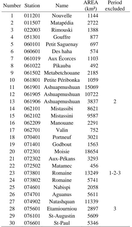
The data used in this study are the daily flows of 30 stations from the Côte-Nord region of the province of Québec (Canada), from the years 1950 to 2007, provided by Hydro-Québec Research Institut. Because the number of stations is already small, no additional constraints were added on the minimum number of years. Record lengths vary between 10 and 51 years. The variables used were the autumnal flood peak and volume quantiles (section 4.1).

3.2 Physiographical and meteorological data

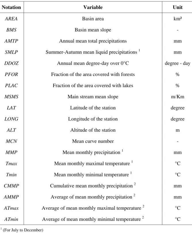
For each station, several physiographical and meteorological variables are available from Environnement Canada (Table 1). To ensure that all autumnal phenomena are taken into account, the data of the mean monthly precipitation (MMP) and the mean monthly maximal and minimal temperature (Tmax and Tmin) for July to December were combined. The cumulative mean

29

monthly precipitation (CMMP), the average of the mean monthly precipitation (AMMP) and the averages of the mean monthly maximal and minimal temperature (ATmax and ATmin) were obtained for each combination of months, C , where n=6 and k=1,…,n. These values are noted by k_n the numbers of the months used to calculate them. For example, the average of the mean minimal temperatures of July and August is noted ATmin07-08.

4. Methodology

4.1 Autumnal flood quantiles

The variables of interest are the flood peak and volume quantiles. To obtain them, three steps were followed:

- Determine the period during which autumnal floods occur, - Extract the flood peak and volume series,

- Carry out the at-site flood frequency analysis.

The first step consisted of an exploratory analysis of the annuals hydrographs with advice from meteorologists. To test the robustness of the models, three periods were studied: September 1st to December 15th (period 1), July 1st to December 15th (period 2) and July 1st to August 31st (period 3). For each period, the flood peak and the flood volume of each station, for each year, were extracted. The peak is the maximum flow recorded during the period (in m³/s) and defines the flood of interest. The boundaries of the flood are determined by the detection of a reversal of the slope flow, but an adjacent flood is included if there are less than 15 days between his peak and the maximum peak. The volume is the integral of the flood (in Mm³).

30

The Wald–Wolfowitz test for independence, the Wilcoxon test for homogeneity and the Mann–Kendall rank correlation test for trend detection were applied on hydrometric data to ensure quality. Station 13 (Table 2) failed every test for period 2 and station 28 failed the stationary and homogeneity tests for period 3. Station 23 was removed from all periods because it was identified as a station of interest for further case study. A total of 29, 28 and 28 stations were available for the three periods, respectively (Table 2). It is important to mention that for some stations with short records, the Wilcoxon test was not conclusive.

Local estimates of flood quantiles were then obtained using the most appropriate statistical distribution for each period of the study. The Akaïki criterion was used to choose between the following distributions: Normal (N), Two-Parameter Normal (LN2), Three-Parameter Log-Normal (LN3), Exponential (EX2), Gumbel (GUM), General Extreme Value (GEV), Weibull (W2), Gamma (G2), Inverse Gamma (IG2), Three-Parameter Generalised Gamma (GG3), Pearson Type III (P3), Log-Pearson Type III (LP3) and Halphen Type A (HA). Finally, the hydrologic variables were the at-site flood peak (Q ) and volume (_T V ) quantiles corresponding to the return _T periods T = 10, 20, 50, 100, 1000 and 10000 years. The specific quantiles (flood quantiles standardized by the basin area), noted QS and _T VS , were used to eliminate the scale effect (Eaton _T et al., 2002) and were compared to the absolute quantiles (not standardized). The local estimate of return period of 10000 years obtained from sets of 10 to 15 years may introduce errors in the model.

4.2 Intercomparison criteria

A jackknife resampling procedure was developed in which each station was removed in-turn from the hydrologic network and assumed ungauged. At each stage of the procedure, the basin

31

that was removed was considered a target-basin. The estimates of the quantiles were then obtained at that site by using the remaining basins and by considering the two previously described approaches: CCA and UCK. Four criteria were adopted to study the relative performances of the two regionalization approaches. These are the mean bias (BIAS), the relative mean bias (BIASr), the root mean square error (RMSE) and the relative root mean square error (RMSEr), which can be written as follows:

(

, ,

)

1 1 BIAS -= =

∑

n _{i R i L} i Y Y n (19) , , 1 , -1 BIASr = ⎛ ⎞ = ⎜_⎜ ⎟_⎟ ⎝ ⎠

∑

n i R i L i i L Y Y n Y (20)

(

, ,

)

2 1 1 RMSE -= =

∑

n _{i R i L} i Y Y n (21) 2 , , 1 , -1 RMSEr = ⎛ ⎞ = ⎜_⎜ ⎟_⎟ ⎝ ⎠

∑

n i R i L i i L Y Y n Y (22)

where Y_{i R,} and Y correspond to the regional and local estimates of the quantiles at station i, _{i L,} respectively, and n is the number of stations. All transformations of the regional estimate, such as standardization by basin area for specific quantiles (section 4.1), were reversed prior to the calculation of the criteria in order to obtain the same unit.

To look at the error at each station, the bias ( B_i), relative bias ( Br_i), root square error ( RSE_i) and relative root square error ( RSEr_i) for station i were defined from the jackknife procedure:

32 , , B_i =Y_{i R}-Y_{i L} (23) , , , -Br_i i R i L i L Y Y Y = (24)

(

)

2 , , RSE_i = Y_{i R}-Y_{i L} (25) 2 , , , -RSEr_i i R i L i L Y Y Y ⎛ ⎞ = ⎜_⎜ ⎟_⎟ ⎝ ⎠ (26)

Equations 9 to 12 are called the mean errors and equations 13 to 16 are called the errors of the jackknife procedure.

5. Results and Discussion

5.1 Variables

The correlation between the physiographical/meteorological variables and the hydrological variables was thoroughly studied. The physiographical/meteorological variables are chosen according to their correlation degree with the flood quantiles and by taking care that there is no co-linearity between them. Four variables were considered with the absolute quantiles and three with the specific quantiles. The best results were obtained with the basin area (AREA), the summer-autumn mean liquid precipitations (SMLP) (for the absolute quantiles only), the fraction of the basin area covered by lakes (PLAC) and the average of the mean July, August and September maximal temperatures (ATmax07-08-09). The variables were the same for all periods. The removal of the precipitation variable was due to its high correlation with the temperature variable. Because CCA requires variable normality, a logarithmic transformation was applied to the variables prior to the analysis.

33

5.2 Application of the CCA method

Absolute quantiles

For each period, different multiple regression models were tested, with the neighborhood defined by CCA. For the three periods, the model leading to the best results was the log-linear model:

( )

(

)

(

)

(

)

(

)

( )

(

)

(

)

(

)

(

)

1, 2, 3, 4, 5, 1, 2, 3, 4, 5,

log log log log

log

log log log log

log T T T T T T T T T T T T Q AREA SMLP PLAC ATmax07 - 08 - 09 V AREA SMLP PLAC ATmax07 - 08 - 09 β β β β β γ γ γ γ γ = + + + + = + + + + (27)

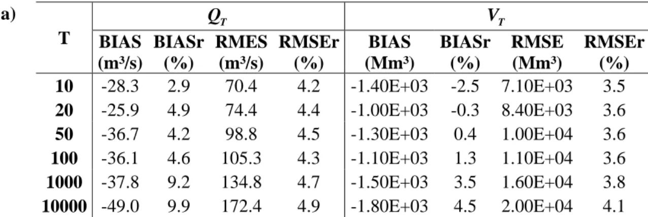
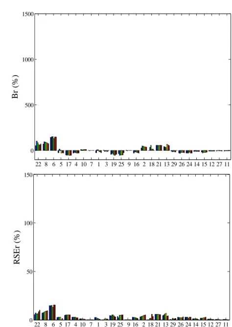
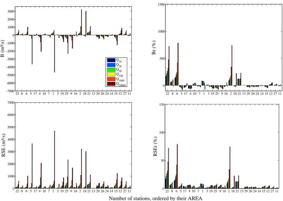
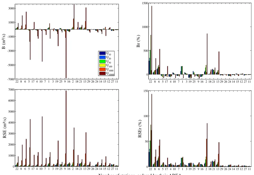
where T is the return period. Figure 1, 2 and 3 present the errors of periods 1, 2 and 3 by station, respectively, for every station i. The errors of Q ( B_{T i}, Br_i, RSE_i and RSEr_i) are shown on the same scale for the three periods and are in ascending order of their AREA. Errors were smaller for period 1 than for the other periods, especially for T = 1000 and 10000 years. The same observations and conclusions held for V , so they are not presented here. _T

Figure 1 permits one to observe that the relative errors ( Br_i and RSEr_i) were greater for small than for large basins. This seems to indicate that physiographical and meteorological variables are less accurate for small basins. The mean errors of the jackknife procedure (BIAS,

BIASr, RMSE and RMSEr) for period 1 are listed in Table 3a. The model performed well, leading to a BIASr lower than 10.0% for Q and lower than 4.5% for _T V , and an RMSEr lower _T than 5.0%. The results permit one to confidently extrapolate the model to other Québec regions for autumnal flood studies, since the model and the variables are the same for every periods. The period should be revised for more accurate results.

34 Specific quantiles

The regional analysis was also carried out on the specific quantiles. Multiple regression models were tested, and the best was again the log-linear model:

(

)

(

)

(

)

(

)

(

)

(

)

(

)

(

)

1, 2, 3, 4,

1, 2, 3, 4,

log log log log

log log log log

T T T T T

T T T T T

QS AREA PLAC ATmax07 - 08 - 09

VS AREA PLAC ATmax07 - 08 - 09

β β β β

γ γ γ γ

= + + +

= + + + (28)

where T is the return period. The three periods were studied, but the results are not presented here, as they are similar to those observed for the absolute quantiles and lead to same conclusions. For period 1, the mean errors of the jackknife procedure on the specific quantiles are shown in Table 3b. To allow for comparison with the absolute quantiles, the estimated specific quantiles were multiplied by their AREA before the calculation of the criteria (see section 4.2). The mean errors of the jackknife procedure are shown in Table 3b. The BIASr was lower than 12.0% for QS and _T lower than 3.5% for VS , and the RMSEr was lower than 4.5% for _T QS and lower than 3.5% for _T

T

VS .

Discussion

A comparison of the absolute and specific quantiles (Table 3a,b) showed that, for the volume, the specific quantiles perform best, except for the return periods of 20, 50, and 100 years, where the BIASr values were better for the absolute quantiles. The BIAS was approximately 10 times smaller for the specific quantiles than for the absolute quantiles. For the peak, the BIAS and RMSEr were smaller for specific quantiles, but the BIASr and RMSE were smaller for absolute quantiles. Exhaustive studies of the errors showed that the peaks of small stations are best

35

estimated with specific quantiles, and the peaks of large station are best estimated with absolute quantiles.

It is preferable to use the specific as opposed to the absolute quantiles. The errors of volume and half errors of peak are better with the specific quantiles than the absolute quantiles. The ACC method leads to BIASr values lower than 12.0% for Q and lower than 3.5% for _T V , and _T RMSEr values lower than 4.5% for Q and lower than 3.5% for _T V . _T

5.3 Application of the UCK method

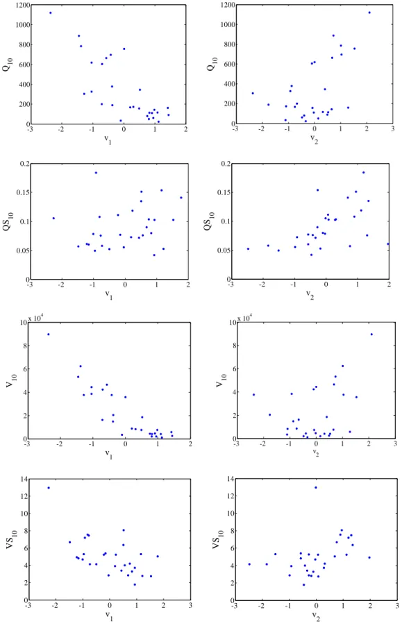
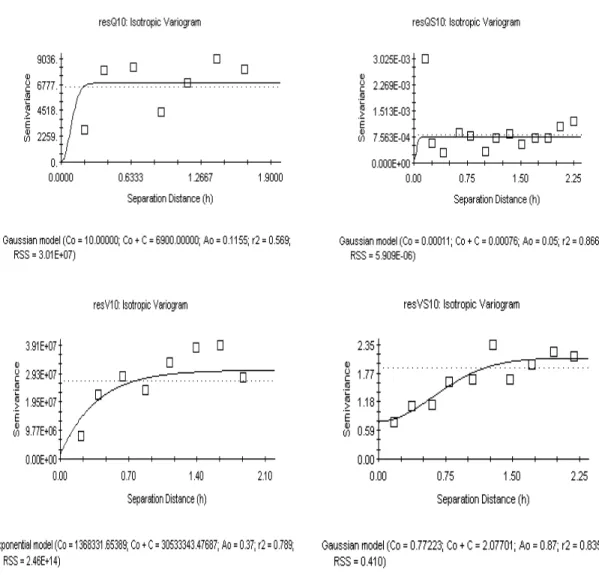
To ensure the ability to compare the UCK method with the CCA method, the same explicative variables were used with the UCK method to construct the canonical physiographical space. Period 1 was already identified as the best, so this part of the study concentrated on it. A comparison of the absolute and specific quantiles was again carried out. Figure 4 presents an example of the quantiles (Q , _T QS , _T V and _T VS ) versus the two physiographical canonical _T variables (v and ₁ v ) for T = 10 years. Quantiles were not stationary over the physiographical ₂ space. The same phenomenon was observed for all return periods. The trend was quantified and removed with a second-order regression:

(

)

2 2

1,T, 2,T ( 1,T 2,T* 1,T 3,T* 2,T 4,T* 1,T 5,T* 2,T)

v v = a +a v +a v +a v +a v

A (29)

where A

(

v1,T,v2,T

)

represents the trend of the hydrologic quantiles of the return period T, ai T, are the regression parameters, and v_1,T and v_2,T are the first and second physiographical canonical variables, respectively. A Gaussian model was fitted to all experimental variograms except for V , ₁₀

20

36

variograms and fitted model of each quantile for T = 10 years. The models were selected according to the pattern of the spatial structure shown by the experimental variograms. Due to the very small number of stations and the high variability between the quantiles of each station, the experimental variograms were hard to adjust. Despite this, good results were obtained.

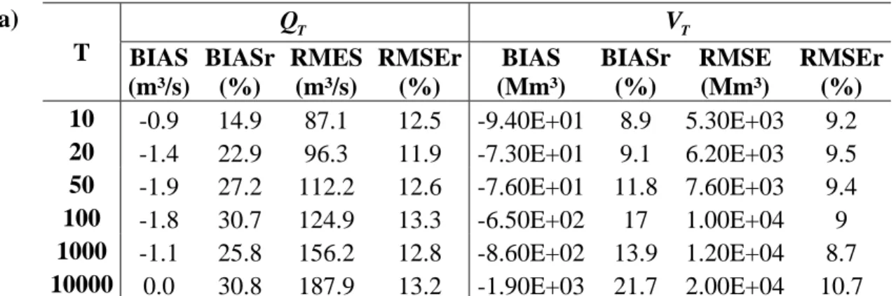
The mean errors are presented in Table 4. BIAS and RMSE were systematically better for the absolute quantiles, and BIASr and RMSEr were better for the specifics quantiles, for peak as well as for volume. An exhaustive study showed that some stations were always problematic, such as station 22 for the absolute quantiles and station 24 for the specific quantiles. The error on station 22, which has a small basin of 456 km², was high, so the relative errors were very important, and the opposite phenomenon was observed for station 24, which has a basin of 5741 km². The exhaustive study also showed that the differences between the absolute errors are negligible in comparison to the differences between the relative errors. Furthemore, the local estimate of those two basins can be inaccurate, having record lengths of 10 and 12 year. Even if the results are not as evident as for the CCA method, the specific quantiles led to better results than the absolute quantiles. The BIASr was lower than 15% for the peak quantiles and lower than 5% for the volume quantiles, and the RMSEr was lower than 7%.

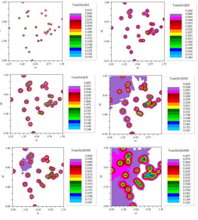
The UCK method has the particularity of enable drawing of errors maps. These maps can take into account the local and regional errors, as well as the sampling errors if they are known. Figures 6 and 7 show the maps of the local and regional standard deviation (Std) for QS and _T VS _T in the physiographical space for all T. The maps changed slightly as T grew. For QS , Std _T increased quickly near the observed data and was approximately the same everywhere else, but the increase became slower as T grew. For VS , Std was more continuously distributed in the T

37

5.4 Comparison results

The comparison of the regional estimation by CCA and UCK using specific quantiles (Table 3 and 4) demonstrates that the CCA method leads generally to better results. There are two exceptions: the BIAS of the peak and the BIASr of the volume. The values of the BIASr indicate that the peak quantiles are systematically overestimated, but the volume quantiles are not, especially with the UCK method. The differences in the BIAS values, which generally indicate an underestimation, for the two cases seem to indicate that the large basins are generally underestimated and the small basins are overestimated. In general, the errors on the small basins are more important. This impression is supported by an exhaustive study of the errors of each basin regarding their basin area. The results in Table 4 indicate that the relative performance of the UCK method on the volume quantiles improved with the increasing return period; the BIASr and the RMSEr decreased when the return period was growing.

The CCA approach performed better than the UCK approach. Nevertheless, the results are based on only 29 stations, which is a small sample size for a regional analysis. It seems that the UCK method is more affected by the sample size. Furthermore, the differences between results are small, and the UCK method permits one to construct maps of the errors with all of the errors taken into account (Figures 6 and 7). This represents an advantage of the UCK method which may motivate its use instead of the CCA method, despite its inferior performance.

6. Conclusions and Future Work

The study of the CCA and UCK methods applied to the autumnal flood was carried out on a set of 29 stations from the Côte-Nord region (Québec, Canada). Three periods during which the autumnal floods generally occur were tested to determine the peak and volume from September 1st

38

to December 15th. This result suggests that there is a difference between summer and autumnal floods and they should be studied separately in the future. Nevertheless, the model performs well even if summer and autumnal are taken together.

The application of the CCA model indicated a temporal robustness for the determination of the explicative variables as well as for the regression model. A comparison of the absolute and specific quantiles demonstrated the superiority of the specific quantiles for both methods, but the advantage was not as strong as expected. A comparison of the two methods using a jackknife resampling procedure led to very similar results, but with the best performance reached by the CCA method. It seems that the UCK method is more affected by the small number of stations.

This study is a first step in the understanding of the autumnal flood in a four-season region. The application of these two methods to a more considerable database should be performed in the future to confirm the results. Since the UCK method does not require independent variables, the number of variables is not limited. Future work should be dedicated to testing how many variables can be introduced in the model and whether this leads to better results.

7. Acknowledgement

The financial support provided by Hydro-Québec and the Natural Sciences and Engineering Research Council of Canada (NSERC) is gratefully acknowledged. The authors wish also to thank Salaheddine El Adlouni, Fateh Chebana and Luc Perreault for their assistance.

8. References

Burn D.H. (1990). "Evaluation of Regional Flood Frequency Analysis with a Region of Influence Approach." Water Resour. Res., 26, 2257–2265.

39

Chokmani K., Ouarda T. (2004). "Physiographical space-based kriging for regional flood frequency estimation at ungauged sites." Water Resour. Res., 40.

Dalrymple T. (1960). "Flood frequency analysis." U.S. Geol. Surv. Water Supply Pap., 1543-A Eaton B., Church M., Ham D. (2002). "Scaling and regionalization of flood flows in British

Columbia, Canada." Hydrol. Process., 16, 3245-3263.

GREHYS (1996a). "Presentation and review of some methods for regional flood frequency analysis." J. Hydrol., 186, 63-84.

GREHYS (1996b). "Inter-comparison of regional flood frequency procedures for Canadian rivers." J. Hydrol., 186, 85-103.

Grover P.L., Burn D.H., Cunderlik J.M. (2002). "A comparison of index flood estimation procedures for ungauged catchments." Can. J. Civil Engng, 29, 734-741.

Kamali Nezhad M., Chokmani K., Ouarda T.B.J.M., El Adlouni S. (2009). "Regional flood frequency analysis using universal kriging in physiographical space." Submitted to Water Resour. Res.

Muirhed R.J., 1982 Aspects of Multivariate Statistical Theory (Wiley, New York).

Ouarda T.B.M.J., Haché M., Bruneau P., Bobée B. (2000). "Regional flood peak and volume estimation in northern Canadian basin." J. Cold Reg. Engng, 14, 176-191.

Ouarda T.B.M.J., Girard C., Cavadias G.S., Bobee B. (2001). "Regional flood frequency estimation with canonical correlation analysis." J. Hydrol., 254, 157-173.

40

Ouarda T.B.M.J., Cunderlik J.M., St-Hilaire A., Barbet M., Bruneau P., Bobee B. (2006). "Data-based comparison of seasonality-"Data-based regional flood frequency methods." J. Hydrol., 330, 329-339.

Ouarda T.B.M.J., Ba K.M., Diaz-Delgado C., Carsteanu A., Chokmani K., Gingras H., Quentin E., Trujillo E., Bobee B. (2008). "Intercomparison of regional flood frequency estimation methods at ungauged sites for a Mexican case study." J. Hydrol., 348, 40-58.

Pandey G.R., Nguyen V.T.V. (1999). "A comparative study of regression based methods in regional flood frequency analysis." J. Hydrol., 225, 92-101.

Shu C., Ouarda T. (2007). "Flood frequency analysis at ungauged sites using artificial neural networks in canonical correlation analysis physiographic space." Water Resour. Res., 43. Shu C., Ouarda T.B.M.J. (2008). "Regional flood frequency analysis at ungauged sites using the

41

Table 1: List of all physiographical and meteorological variables considered in this study.

Notation Variable Unit

AREA Basin area km²

BMS Basin mean slope -

AMTP Annual mean total precipitations mm

SMLP Summer-Autumn mean liquid precipitations 1 mm

DDOZ Annual mean degree-day over 0°C degree - day

PFOR Fraction of the area covered with forests %

PLAC Fraction of the area covered with lakes %

MSMS Main stream mean slope m/Km

LAT Latitude of the station degree

LONG Longitude of the station degree

ALT Altitude of the station m

MCN Mean curve number -

MMP Mean monthly precipitation 1 mm

Tmax Mean monthly maximal temperature 1 °C

Tmin Mean monthly minimal temperature 1 °C

CMMP Cumulative mean monthly precipitation 2 mm

AMMP Average of mean monthly precipitation 2 mm

ATmax Average of mean monthly maximal temperature 2 °C

ATmin Average of mean monthly minimal temperature 2 °C

1

(For July to December)

2

42

Table 2: List of the 30 hydrometric stations used in the study, with their basin area and the stations

excluded for each period. Period 1 is September 1st to December 15th, period 2 is July 1st to December 15th and period 3 is July 1st to August 31st.

Number Station Name AREA

(km²) Period excluded 1 011201 Nouvelle 1144 2 011507 Matapédia 2722 3 022003 Rimouski 1388 4 051301 Gouffre 877 5 060101 Petit Saguenay 697 6 060601 Des haha 574 7 061019 Aux Écorces 1103 8 061022 Pikauba 492 9 061502 Metabetchouane 2185 10 061801 Petite Péribonka 1059 11 061901 Ashuapmushuan 15069 12 061905 Ashuapmushuan 10722 13 061906 Ashuapmushuan 3837 2 14 062101 Mistassibi 8621 15 062102 Mistassini 9587 16 062209 Manouane 2291 17 062701 Valin 752 18 070401 Portneuf 3021 19 071401 Godbout 1563 20 072301 Moisie 18654 21 072302 Aux-Pékans 3293 22 072502 Matamec 456 23 073801 Romaine 13249 1-2-3 24 073802 Romaine 5741 25 074601 Nabispi 2058 26 074701 Aguanus 5611 27 074902 Natashquan 11339 28 075601 Etamiourniou 2897 3 29 076101 St-Augustin 5609 30 076601 St-Paul 5346

43

Table 3: Comparative results of a) absolute quantiles (Q and _T V ) and b) specific quantiles _T

(QS and _T VS ) for regional analysis with CCA on period 1. _T

a) T T Q V_T BIAS (m³/s) BIASr (%) RMES (m³/s) RMSEr (%) BIAS (Mm³) BIASr (%) RMSE (Mm³) RMSEr (%) 10 -28.3 2.9 70.4 4.2 -1.40E+03 -2.5 7.10E+03 3.5 20 -25.9 4.9 74.4 4.4 -1.00E+03 -0.3 8.40E+03 3.6 50 -36.7 4.2 98.8 4.5 -1.30E+03 0.4 1.00E+04 3.6 100 -36.1 4.6 105.3 4.3 -1.10E+03 1.3 1.10E+04 3.6 1000 -37.8 9.2 134.8 4.7 -1.50E+03 3.5 1.60E+04 3.8 10000 -49.0 9.9 172.4 4.9 -1.80E+03 4.5 2.00E+04 4.1 b) T T QS VS_T BIAS (m³/s) BIASr (%) RMES (m³/s) RMSEr (%) BIAS (Mm³) BIASr (%) RMSE (Mm³) RMSEr (%) 10 -16.6 7.4 98.7 4 -2.80E+02 2.2 4.60E+03 3 20 -11.2 9.8 104.4 4.1 -1.50E+02 3 5.30E+03 3 50 -10.9 9.6 108.6 4 -3.90E+02 2.6 6.70E+03 3 100 -11.4 10.1 118.7 4.1 -5.40E+02 2.3 7.50E+03 3 1000 -10.4 11.3 151 4.2 -1.10E+03 3 1.10E+04 3.1 10000 -8.7 11.6 181.4 4.3 -8.60E+02 3.5 1.60E+04 3.2

44

Table 4: Comparative results of a) absolute quantiles (Q and _T V ) and b) specific quantiles _T

(QS and _T VS ) for regional analysis with UCK on period 1. _T

a) T T Q V_T BIAS (m³/s) BIASr (%) RMES (m³/s) RMSEr (%) BIAS (Mm³) BIASr (%) RMSE (Mm³) RMSEr (%) 10 -0.9 14.9 87.1 12.5 -9.40E+01 8.9 5.30E+03 9.2 20 -1.4 22.9 96.3 11.9 -7.30E+01 9.1 6.20E+03 9.5 50 -1.9 27.2 112.2 12.6 -7.60E+01 11.8 7.60E+03 9.4 100 -1.8 30.7 124.9 13.3 -6.50E+02 17 1.00E+04 9 1000 -1.1 25.8 156.2 12.8 -8.60E+02 13.9 1.20E+04 8.7 10000 0.0 30.8 187.9 13.2 -1.90E+03 21.7 2.00E+04 10.7 b) T T QS VS_T BIAS (m³/s) BIASr (%) RMES (m³/s) RMSEr (%) BIAS (Mm³) BIASr (%) RMSE (Mm³) RMSEr (%) 10 -15.6 8.6 121.7 4.1 -3.50E+03 -3.1 2.20E+04 6.4 20 -2.7 10.4 111.8 4.3 -3.50E+03 -2.5 2.40E+04 5.9 50 3.3 11.7 145.3 4.7 -3.80E+03 -1.3 2.60E+04 5.7 100 8.2 13.4 164 5 -3.90E+03 -0.8 2.80E+04 5.6 1000 0.4 12.5 213.1 5 -4.10E+03 0.3 3.50E+04 5.3 10000 12.4 14.9 252 5.3 -4.00E+03 0.8 4.10E+04 4.9

45

Figure captions

Figure 1: B_i, Br_i, RSE_i and RSEr_i of Q , for all values of T, for each station i, for period 1, _T with the ACC method. ...47 Figure 2: B_i, Br_i, RSE_i and RSEr_i of Q , for all values of T, for each station i, for period 2, _T

with the ACC method. ...48 Figure 3: B_i, Br_i, RSE_i and RSEr_i of Q , for all values of T, for each station i, for period 3, _T

with the ACC method. ...49 Figure 4: Q , ₁₀ QS , ₁₀ V , ₁₀ VS versus ₁₀ v and ₁ v . ...50 ₂ Figure 5: Experimental variograms for Q , ₁₀ QS , ₁₀ V , ₁₀ VS . ...51 ₁₀ Figure 6: Map of local and regional standard deviations of QS with the KCU method, for _T

T = 10, 20, 50, 100, 1 000 and 10 000 years. ...52 Figure 7: Map of local and regional standard deviations of VS with the KCU method, for _T

47 22 8 6 5 17 4 10 7 1 3 19 25 9 16 2 18 21 13 29 26 24 14 15 12 27 11 -7000 -5000 -3000 -1000 1000 3000 B (m³ /s ) Q 10 Q₂₀ Q 50 Q₁₀₀ Q 1000 Q₁₀₀₀₀ 22 8 6 5 17 4 10 7 1 3 19 25 9 16 2 18 21 13 29 26 24 14 15 12 27 11 0 500 1000 1500 Br (% ) 22 8 6 5 17 4 10 7 1 3 19 25 9 16 2 18 21 13 29 26 24 14 15 12 27 11 0 1000 2000 3000 4000 5000 6000 7000 RSE (m³/ s) 22 8 6 5 17 4 10 7 1 3 19 25 9 16 2 18 21 13 29 26 24 14 15 12 27 11 0 50 100 150 RSE r (% )

Number of stations, ordered by their AREA

Figure 1: B_i, Br_i, RSE_i and RSEr_i of Q , for all values of T, for each station i, for period 1, with the ACC method. Stations are in ascending order _T

48 22 8 6 5 17 4 10 7 1 3 19 25 9 16 2 18 21 13 29 26 24 14 15 12 27 11 -7000 -6000 -5000 -4000 -3000 -2000 -1000 0 1000 2000 3000 B (m ³/ s) Q₁₀ Q₂₀ Q₅₀ Q₁₀₀ Q₁₀₀₀ Q₁₀₀₀₀ 22 8 6 5 17 4 10 7 1 3 19 25 9 16 2 18 21 13 29 26 24 14 15 12 27 11 0 500 1000 1500 Br ( % ) 22 8 6 5 17 4 10 7 1 3 19 25 9 16 2 18 21 13 29 26 24 14 15 12 27 11 0 1000 2000 3000 4000 5000 6000 7000 RSE ( m ³/ s) 22 8 6 5 17 4 10 7 1 3 19 25 9 16 2 18 21 13 29 26 24 14 15 12 27 11 0 50 100 150 RSE r (% )

Number of stations, ordered by their AREA

Figure 2: B_i, Br_i, RSE_i and RSEr_i of Q , for all values of T, for each station i, for period 2, with the ACC method. Stations are in ascending order _T

49 22 8 6 5 17 4 10 7 1 3 19 25 9 16 2 18 21 13 29 26 24 14 15 12 27 11 -7000 -5000 -3000 -1000 1000 3000 B (m³/ s) Q₁₀ Q 20 Q₅₀ Q 100 Q₁₀₀₀ Q₁₀₀₀₀ 22 8 6 5 17 4 10 7 1 3 19 25 9 16 2 18 21 13 29 26 24 14 15 12 27 11 0 500 1000 1500 Br (% ) 22 8 6 5 17 4 10 7 1 3 19 25 9 16 2 18 21 13 29 26 24 14 15 12 27 11 0 1000 2000 3000 4000 5000 6000 7000 RSE (m³/ s) 22 8 6 5 17 4 10 7 1 3 19 25 9 16 2 18 21 13 29 26 24 14 15 12 27 11 0 50 100 150 RSE r (% )

Number of stations, ordered by their AREA

Figure 3: B_i, Br_i, RSE_i and RSEr_i of Q , for all values of T, for each station i, for period 3, with the ACC method. Stations are in ascending order _T

50 -3 -2 -1 0 1 2 0 200 400 600 800 1000 1200 v₁ Q 10 -3 -2 -1 0 1 2 3 0 200 400 600 800 1000 1200 Q 10 v₂ -3 -2 -1 0 1 2 0 0.05 0.1 0.15 0.2 v₁ QS 10 -3 -2 -1 0 1 2 0 0.05 0.1 0.15 0.2 QS 10 v₂ -3 -2 -1 0 1 2 0 2 4 6 8 10x 10 4 V 10 v₁ -3 -2 -1 0 1 2 3 0 2 4 6 8 10x 10 4 V 10 v 2 -3 -2 -1 0 1 2 3 0 2 4 6 8 10 12 14 VS 10 v₁ -3 -2 -1 0 1 2 3 0 2 4 6 8 10 12 14 VS 10 v₂

51

52

Figure 6: Map of local and regional standard deviations of QS with the KCU method, for _T