Trade is not necessary for agglomeration to arise

HAL Id: hal-01526534

https://hal.archives-ouvertes.fr/hal-01526534

Submitted on 23 May 2017

HAL is a multi-disciplinary open access

archive for the deposit and dissemination of

sci-entific research documents, whether they are

pub-lished or not. The documents may come from

teaching and research institutions in France or

L’archive ouverte pluridisciplinaire HAL, est

destinée au dépôt et à la diffusion de documents

scientifiques de niveau recherche, publiés ou non,

émanant des établissements d’enseignement et de

recherche français ou étrangers, des laboratoires

Trade is not necessary for agglomeration to arise

Kristian Behrens

To cite this version:

Kristian Behrens. Trade is not necessary for agglomeration to arise. [Research Report] Laboratoire

d’analyse et de techniques économiques(LATEC). 2003, 30 p., figures, bibliographie. �hal-01526534�

LABORATOIRE D'ANALYSE

ET DE TECHNIQUES ÉCONOMIQUES

UMR5118 CNRS

Pôle d'Économie et de Gestion

UNIVERSITE

DE BOURGOGNE

2,

bd Gabriel-

-

F

Dijon cedex

-

T

él.

-

Fax

Courrier électronique: secretariat.latec@u-bourgogne.fr ISSN : 1260-8556

n° 2003-07

Trade is not necessary

for agglomeration to arise

Kristian BEHRENS

Kristian Behrens * LATEC

U n iv e r s ite d e B o u r g o g n e

April 9th 2003

Trade is not necessary for agglom eration to arise

* LATEC, Université de Bourgogne, Pôle d ’Économie et de Gestion, B.P. 26611, 21066 Dijon CEDEX, France (email: K r is tia n B e h r e n s Q a o l.c o m ). The

author is indebted to J acques-François Thisse, Christian Michelot and Jean- Marie Huriot as well as participants a t LASERE Workshop (CORE, Belgium) and LATEC Workshop (Dijon, France) for valuable comments and suggestions. P aper presented at the 49th North American meeting of the Regional Science Association International in San Juan (Puerto Rico), November 14th - 16th 2002.

Abstract

We develop a spatial general equilibrium model in which the absence of trade is an endogenous outcome and we show that trade is not a necessary condition for agglomeration to arise. More precisely, extending the model developed by Ottaviano et al. [13], we show that equilibria without trade differ significantly from those obtained in the presence of trade. Somewhat surprisingly, equilibrium structures without trade are richer than those with trade, since partial agglomeration becomes a feasible outcome. Equilibria now depend on the ratio of mobile to immobile factors and an increase in that ratio triggers a process of spatial agglomeration.

Résumé

Nous développons un modèle d’équilibre général spatial dans lequel l’absence de commerce est un résultat endogène et nous montrons que le commerce n’est pas une condition nécessaire à l’agglomération. Plus précisément, nous étendons le modèle de Ottaviano et al. [13] et nous montrons que les équilibres sans commerce diffèrent significativement de ceux obtenus avec commerce. Il est surprenant que les structures d’équilibre sans commerce sont plus riches que celles avec, puisque l’agglomération partielle peut se produire. Les équilibres dépendent du ratio de facteurs mobiles et immobiles; un ac­ croissement de ce ratio mène à un processus d’agglomération spatial.

Keywords : agglomeration, trade, imperfect competition, comer solutions JE L Classification : D l l , F12, L13, R12

1. Introduction

Since the Industrial Revolution, the transport costs of goods have decreased enor­ mously. The 19th century witnessed a first ‘revolution’ in transportation technologies, with the advent of railroads and steamships, while the 20th century witnessed a second

‘revolution’ with the rapid development of air freight and mass communication tech­ nologies. Those transport revolutions were accompanied by a rapid increase in both the volume of trade and the size of urban structures (see Bairoch [1]). Since about a decade, and the seminal paper by Krugman [11], economists have started to investigate more closely the various links between transport costs, trade and agglomeration in a spatial general equilibrium context. One of the fundamental results of the so-called ‘new’ economic geography states that agglomeration usually arises when transport costs are sufficiently low, while dispersion is the equilibrium outcome when transport costs are high (see Fujita et al. [5], Krugman [11], Ottaviano et al. [13] and Puga [15]). This result is well summarized by Henderson et al. [10] who state that, “if transport

and communication costs are very high then activity must be dispersed”. Therefore,

even if trade is not a sufficient condition, it seems that trade is at least a necessary condition for agglomeration to occur. In the present paper, we investigate if there can

be agglomeration without trade or if the absence of trade always implies the dispersion

of economic activity. To put it differently, we would like to know if trade is really a

necessary condition for agglomeration or if agglomerated no-trade equilibria exist. We

think it is worth mentioning right from the start that, as shown in this paper, trade is not

a necessary condition for agglomeration to occur and that the equilibrium structures

are, somewhat surprisingly, even richer when there is no trade than in the presence of trade.

It is a bit surprising that the question concerning the possibility of agglomeration without trade has, to the best of our knowledge, not been addressed in economic geog­ raphy. Indeed, one of the striking features of the space-economy is the empirical fact that only a small fraction of all goods produced in an industry is available in any one particular location. This fact, which we believe is about as characteristic o f a spatial

economy as the uneven distribution o f production, has not received the attention it

deserves (see Tabuchi and Thisse [17] for an exception). A closer look at the main canonical models of the ‘new’ economic geography (Krugman [11] or Ottaviano et al. [13]) reveals that those models are all build, either explicitly or implicitly, on the assumption that each economic agent consumes a strictly positive quantity of all goods produced in the economy, no matter how firms and consumers are distributed in space. This clearly highlights the fact that those models are not suited to deal with the spatial location of nontradeables, since they assume that all goods are tradeable. Hence while, as Wong [18] argues, “the theory o f international trade has paid too much attention to

trade in goods and far too little to factor mobility”, it seems that the ‘new’ economic

geography suffers from the opposite deficiency by systematically assuming that goods are mobile. Yet, in many countries, despite the secular decline in transportation costs, several goods and most services are only available in major metropolitan regions (think of most buisness-to-consumer services). Krugman [12] neatly explains that we, some­ what paradoxically, observe that “while we ship manufactured goods back and forth

with unprecedented abandon, such “tradeables” constitute a steadily shrinking share o f our economy”. How does the spatial immobility of some outputs and the resulting

absence of interregional trade in them affect the spatial equilibrium configurations? In order to tackle this question and to shed some light on the possible necessity of trade in the agglomeration process, we move away from the constant elasticity of substitution (CES) framework usually used in the literature. Indeed, this framework implies that there is always at least some bilateral interregional trade (see Fujita et al. [5], Krugman [11] and Puga [15]).1 An alternative modeling strategy is proposed by Ottaviano et al. [13], who have shown that the core-periphery model can be analyzed

1 Since the CES approach is analytically unable to deal with the case in which certain goods are not bought in certain locations, in choosing this framework we implicitly accept the fact that all goods are consumed everywhere, which clearly contradicts our main point of interest. In order to apply the CES to cases with corner solutions we have to use a translated CES function (the traditional CES never allows for that type of solution) (see Deaton and Muellbauer [4]). This translated function, which has been used in applied demand theory and

in a much clearer and analytically tractable fashion with the help of the quadratic utility. While the qualitative results are similar to those obtained in the CES core-periphery model, those authors have shown that several drawbacks of the CES are overcome by the quadratic utility: solutions are in closed-form and there is no need for numerical simulation, the economic meaning of the various parameters is disentangled and the artifical flavor of the particular consequences of the iso-elastic approach disappear. Ottaviano et al. [13] especially show that the demand functions and equilibrium prices now depend on all the fundamentals of the model (including the distribution of firms in space), a result which is more in line with what is known in spatial pricing and demand theory. More important, as shown in Section 2, the quadratic utility is compatible with a simple analytical approach to demand systems with corner solutions. Thus this modeling framework allows us to conveniently addressed the questions concerning the regional availablity of goods and possible equilibria when there is no trade.

The remainder of this paper is organized as follows. In Section 2, we develop an analytical framework that helps us tackle the question of which firms are active in which markets. In Section 3, we apply this framework to the general equilibrium model initially developed by Ottaviano et al. [13]. We show that agglomeration can arise even in the absence of trade, which highlights the fact that trade is not a necessary

condition fo r agglomeration to occur. Section 4 offers some conclusions and points

towards future research directions.

2. Q u a d ratic utility, corner solutions and firms

One approach to consumer problems that allows for both interior and comer solutions with clear-cut analytical results is that of the quadratic utility. Recent works in economic geography, though focusing exclusively on the case of interior solutions, have shown that this kind of modelization may actually be analytically superior to the traditional CES approach (refer to Ottaviano et al. [13] and Ottaviano and Thisse [14]). The basic quadratic utility problem, with a mass of N differentiated varieties, can be stated as follows,

V>q)<

m axX0)I a

f N

s.t. / p(i)x(i)di + xq = w + 0o

^0

where the price of the homogenous good xq is taken as the numéraire, 0o is the initial endowment in good x 0 and a > 0 and fi > 7 > 0 are parameters. One should note

that the positivity constraints on demands x(i) are (as almost always in economics) implicit in this kind of formalization, since one assumes that all varieties will be consumed at the optimum. Since we want to examine the incidence on the spatial equilibrium configurations of certain firms not operating in certain markets, we have to take the comer solutions of (Vq) explicitly into consideration. In order to solve

(Vq) easily, we substitute the constraint into the objective function. This yields an unconstrained optimization problem which, since the objective is quadratic in x , has first order conditions given by a linear system of equations

for all i e [0, N]. In what follows, we set e := /? — 7 for notational convenience.

The parameter e can be interpreted as a substitutability parameter between varieties. Varieties become perfect substitutes in the case in which ¡3 —►7 (i.e. when e —> 0) and

they become independent in the case in which 7 0 (i.e. when t ¡3). The demands

(2) can be rewritten in a more compact way as

Straightforward resolution of conditions (1) yields the demand functions

a)

'N

p ( j) d j (2)

x*(i) = a — (b -f cN)p(i) + cP (i), (3) where a, b and c are positive coefficients, given by

and where

a 1 7

a = --- —-, b = --- —— and c = —--- —

e + N7 e H- N 7 e(e + N'y)

(

4

)

(5) is an aggregate price index of the differentiated industry. As one can see from (3), demand for variety i is decreasing at a constant rate — (b + cN) with respect to own price p(i). This implies that there is a cut-off price beyond which demand is no longer positive. Using (3), we see that demand for variety i is positive if and only if

i.e. if the price p(i) charged by firm i is lower than the cut-off price p(i)y whose analytical expression is quite easily established. As one can see from (6), firm i is more likely to have a positive demand if competition is mild (hence if N is small), if goods are bad substitutes (hence if c is small) and if market-size is large (as noticed by Belleflamme et al. [2] and Ottaviano and Thisse [14], the parameter a, and hence a, can be interpreted in terms of market-size). Since we are interested in both corner and interior solutions, we integrate the positivity constraints indirectly into the demand functions in order to ensure that demands are non-negative for all prices (refer to the appendix for a mathematical justification of this approach). The demands (3) can be redefined in extended form as

where [/]+ denotes the positive part of / . Expression (7) shows that the extended demand functions are piecewise affine, convex and not differentiable. Being convex, the functions (7) allow for directional derivatives everywhere. Those are given by

(

)

x*(i) = [a — (b + cN)p(i) + cP(i)] + (7)

b -f cN if p(i) < p(i)

0 if p(i) > p(i) (8)

and

f — b — cN if p(i) < p(i)

X*r(i) = \

(9)

1 0 if p ( i ) > P ( i )

where the subscripts I and r refer to the left- and right-hand derivatives respectively. Using the well-known equalities max { x ^ x } } = § (# i + x 2) + — x 2\ and [/]+ = max {0, / } , an alternative expression for x*(i) is finally given by

ar*(z) = | [a - (b + cN)p(i) + cP(i)] 4- \ \a - (b -1- cN)p{i) + c P (i)|. (10)

Let us turn next to firm’s profit maximization problem. Traditionally, one only focuses on firm’s price selection problem and eliminates one important strategic aspect: firm’s choices concerning the markets in which it wants to be active. As far as we know, this question has not been addressed in a spatial general equilibrium context until now. In order to keep things simple, we do not explicitly incorporate strategic decisions concerning the choice of active markets into our model but we rather treat both the choice o f prices and the ‘choice' of active markets via firm's optimization problem.

This yields a rudimentary and myopic model of firm “behavior” that assumes that each firm is active in each market where it can make at least a short-term zero profit; that most of firm’s real-world decisions concerning markets are essentially based on long-term considerations will be neglected for the sake of tractability. Each firm in our model has two types of markets: active markets in which it can make at least a zero profit and inactive markets in which it cannot profitably operate. We assume that even if a firm is not active in a market, it quotes a fictional price on that market, which can loosely be interpreted as the price consumers would have to pay in order to get the good at that particular location. As Ottaviano and Thisse [14] argue, “it is precisely because in such locations potential prices are either too high for buyers or too low for sellers that the corresponding good is not traded there”.

We assume, as usual in a monopolistic competition context, that each firm pro­ duces a single variety of the differentiated good under increasing returns to scale using

labor only. Each firm has a fixed production cost of <f> units of labor, zero marginal production cost and uses spatial discriminatory pricing. 2 In order to highlight the main forces at work in the model, we start with a simplified setting in this section. Assume there is a single market with a mass of L consumers. Each firm can access this market at a strictly positive unit trade cost r (expressed in terms of the numéraire), which includes all impedements to trade. Firm i ’s profit is given by

7T(i) = L[p(i) - r]x*(i) — w(f>, (11)

where w is the wage rate of labor. The fundamental problem the firm faces when trying to be active in the market is highlighted by (6) and (11). On the one hand, the firm must set a delivered price that is low enough and satisfies (6) in order to have a positive market share; on the other hand, this delivered price must be high enough to allow the firm to cover (part of) the loss in trade costs, as can be seen from (11). It is therefore possible that a firm cannot satisfy simultaneously those two opposing constraints for a given set of parameters, so that it always makes a negative profit in the market. In that case, the profit maximizing solution is to set a price such that the demand it faces is equal to zero. This scenario can, for theoretical convenience, be considered as the firm ‘choosing’ not to be active in the market. When the firm can simultaneously set a price below the shock-off price (6), that is compatible with the level of trade costs (11), it will be able to sell her output and be active in the market.

The maximization of profit (11) with respect to p(i) yields the following left- and right-hand derivatives:

*■«(*) = £[**(*') + (p(i) ~ T)x*j(i)] (12)

< (* ) = L[x*(i) + (p(i) - t)x*'t{i)}. (13) The optimality conditions in the two possible cases (that of the firm being active or not) can be analyzed as follows. First, we know that the condition 0 G [ttJ (z), 7rJ.(i)] is

Unfortunately, our approach in terms of extended demand functions does not allow for analytical resolution of firm’s profit maximization problem under either uniform delivered or mill pricing.

always necessary for p(i) to be a profit maximizing price. Using (8), (9) and (10) in (12) and (13), one can check that this condition trivially holds for all pricesp(i) > p(i), since for those prices consumer demand is equal to zero. In order for the cut-off price (6) (corresponding to the comer solution x*(i)= 0) to be optimal, we have to examine under which conditions

lira M i) — a+ cP(i) — (b + c N ) t < 0. (14)

p(*)<p(»)

In case condition (14) holds, firm’s profit increases monotonically as its price ap­ proaches the cut-off price, which maximizes its profit (stricto sensu this price mini­ mizes firm’s losses on the market). As one can check, (14) holds if and only if r > p (i). Using the definitions of a, band c, given by (4), we can rewrite this condition as

r > ” + (X5)

€ 4- N 7

Condition (15) highlights the fundamental trade-off which determines whether the firm will be active in the market or not. This trade-off depends on the level of trade costs r, the degree of competition in the market (given by P(i) and N ) and the degree of product differentiation (given by e and 7 ). Condition (15) shows that stronger competition (given by a relatively lower P(i) and higher N ) works against firm i

being active in the market. As expected, the competition effect vanishes as varieties become independent (i.e. when 7 -» 0). Stronger product differentiation (e not too close to 0) and higher preference for the differentiated good make conditions (14) and (15) more unlikely to hold, so that firm i will be active in the market. Note that if varieties become perfect substitutes (i.e. when e —► 0), transport costs must be less than the average price of the industry in order for firm i to be active in the market. Finally, as expected, (15) shows that for a given set of parameters, a higher level of trade costs r will make the presence of firm i in the market less likely. All those results agree with what is known in spatial demand theory.

If we turn to the second case r < p(i), so that condition (15) does not hold, the firm can make a positive profit in the market and we hence get interior solutions. If

p(i) < p(i), the profit function (11) is differentiable so that the optimality conditions reduce to

7T'(¿) = a - 2(6 + cN )p(i) + cP(i) + (b-f c N ) t = 0,

which implies that

_* f:\ _ a + ( b + c N )T + c P (*) „ ^

v (,)

“ ---- wTiwj----

(16)

is the profit maximizing price firm i sets on the market. As expected, this price is decreasing with the degree of competition and increasing with both the level of trade costs and the degree of product differentiation.

We have shown in this section that the quadratic utility approach allows us to model in a simple way patterns of demand involving both interior and comer solutions. Depending on both the level o f trade costs and the degree o f competition, certain firms

will be active in certain markets and will not be active in others.This leads to richer configurations than in the traditional models of the ‘new’ economic geography, in which every variety is consumed everywhere. Since the set of active firms in any particular location is determined by both the mass of firms and the aggregate price index in that location, which depends itself on the spatial distribution of firms, we see that the pattern o f demand is endogenously determined by the locational decisions o f

individual economic agents.This approach hence lends itself well to the analysis of

how demand patterns are influenced by, and in return influence, the distribution of economic activities in a spatial general equilibrium context. Firms choose prices that maximize profits and, in doing so, indirectly ‘choose’ in which markets to be active. Therefore, firms’ locational behavior determines which varieties are available in which locations, which in turn determines where other firms locate. This circular aspect is of fundamental importance and drives most of the subsequent results.

3. A gglom eration w ith o u t trad e

In the following developments, we use the same framework and the same notation as Ottaviano et al. [13]. Consider a setting with two regions H and F. Variables associated with each region will be subscripted appropriately. We suppose that there are two production factors in the economy: mobile manufacturing workers (M-workers) which are employed in the manufacturing (resp. the modem) sector and produce a differentiated good under monopolistic competition and increasing returns to scale; and immobile agricultural workers (A-workers) which are employed in the agricultural (resp. the traditional) sector and produce a homogenous good (the numéraire) under perfect competition and constant returns to scale. Let L be the mass of M-workers and A the mass of A-workers. We denote by À G [0,1] the share of M-workers located in region H; the A-workers are assumed to be evenly split between the two regions, each of which accommodates a mass A /2 o i them. Finally, let N be the mass of varieties of the differentiated good produced in the economy. Since we assume that there are no economies of scope, each firm produces one and only one variety, so that N is also equal to the mass of firms in the economy. Assume, for simplicity, that the homogenous good can be traded costlessly. The differentiated good can be traded at no cost in the interior of each region, while there is a strictly positive unit trade cost of r units of the numéraire in order to ship one unit from region H to F and vice versa. Since there are no intra-regional trade costs for M-goods, each M-firm is at least active in the market it has chosen to locate in. A firm located in H (resp. in F) therefore always sells in its

home market H (resp. F) and can, under certain conditions that we explicit later, also sell in its foreign market F (resp. H).

Using the demand functions (7), the demand a firm located in r € {H, F } faces in region s € {H, F} is given by

= [ a - ( b + cN )p „ + CP8} \ (17)

s. 3 Hence, the profit of a firm located in region r E {H , F } is given by

7Tr = P r r x * r ( P r r ) + (prs ~ T)x*a(prs) + (¡m ^J - <jwr

— 7rrr -f 7Trs — (fywr , s y£r (18) where x*r and x*s are the individual demands in the home and foreign market, given by (17), wr is the wage rate in region r and 0 is the fixed labor requirement in terms of mobile production factor L. Let n n = AL/0 and rip — [I — A)L/(f> be the mass of firms (respectively varieties) located in each of the two regions when labor markets clear. In accord with empirical evidence (see Greenhut [8] and Head and Mayer [9]), we assume that firms use a spatial discriminatory pricing policy and set a particular price for each market separately. Hence, firm’s objective function is separable with respect to prices, so that maximization of total profit amounts to maximization of profits on each market separately. The conditions for profit maximization on each market, which are analogous to those discussed in the previous section, are given by

0 6 [(7Trr){ , (^ rr)r] a n d 0 6 [(tT^),' , (tF„ ) ' ] , (1 9 )

where 7rrr and 7rrs are the gross revenues on each separate market. Since a firm located in region r € {H, F} is always active in market r, the solution on its home market is an interior one. Therefore,

* a -f cPr , /rt .

P r r ~ 2(b + c N ) ~ 2Pr ^

is the profit maximizing price a firm located in r sets on its home market, where

a + cPr

Pr ~ b + cN (21)

is the cut-off price in market r 6 {H ,F }. The price (20) depends of course on aggregate market conditions given by the price-index Pr. The solution on firm’s foreign

Q

Since all firms are symmetric, we drop the firm index iin the following developments. Firms therefore only differ by the region they are located in and by the particular variety they produce.

market s e {H, F}, s ^ r can be either interior or comer, depending on whether the firm can profitably be active in this market while being located in region r or not. This is in line with the fact that in order to be a potential export product, the product must be consumed in the home market. As seen in Section 2, being profitably active in s depends on the level of trade costs r and the degree of competition. The larger r

and the fiercer the competition in s, the less likely a firm located in r can profitably enter this market. Indeed, since competition is fierce, prices of substitute varieties that consumers can locally buy from firms in s are relatively low. This implies that if a firm located in r wants to enter market s, it must charge a sufficiently low price in order to capture a strictly positive share of local demand. If trade costs are too high with respect to that price, the firm will always make a negative profit in market $, which simply means that it is not rational for it to be active in that market. Using optimality conditions (19), the first order conditions on the foreign market s yield

where the expressions for the bilateral trade case, when r is sufficiently low, are of course the same as in Ottaviano et al. [13]. Note that the profit-maximizing prices depend on the price aggregates Ph and Pp, which depend themselves on individual prices set by rival firms. In order to determine the equilibrium prices, we use the same approach as Ottaviano et al. [13]. Each firm sets its optimal price taking aggregate market conditions as given, but taken together these aggregate market conditions must be consistent with optimal individual prices. The two regional price-indices of the M-industry are given by

Solving (23) for r € {H ,F } for its fixed-point, using (20) and (22), we obtain the equilibrium price index

(22)

P r = nr p*r(Pr) +n„p*r(Pr), r ,s € { H ,F }, r ■£ s. (23)

Using (24) in (20) and (22), we finally obtain the equilibrium home market price

„ ★ ,

P r r ^ (25)

and the equilibrium foreign market price

P r r + \ i f T < Pr 2P*r if T > p r .

(26)

As one can see from (25), both in the high and in the low trade cost case, the price p*r is a decreasing function of the mass of firms that operate in market r € {H, F}

(recall that n8 = N — nr). This is due to price competition between firms. The main difference is that in the low trade cost case this decrease is linear while it is strictly

convex in the high trade cost case. 4 Hence, competition is weaker in the case of autarky since firms in region r are only subject to local competition while there is no competition from outside. Firms are thus able to maintain higher average prices

in the case o f autarky as n r increases, which suggests that consumers will have less incentive to migrate to region r once the mass n r o f industry in that region gets large

(there is a sort of decreasing effect of price competition with the mass of firms in the local market). As we explain later, this could be one possible reason for the existence of partially agglomerated equilibria in this configuration of the model.

In the remainder of this paper, we focus on the case in which trade costs are ‘high’ in order to show that trade is not a necessary condition fo r agglomeration to

emerge.We believe that the theoretical case of ‘high’ trade costs is as important as the case of ‘low’ trade costs because nobody neither knows for sure what ‘high’ or ‘low’ precisely means is in that type of models nor how it relates to actual trade costs in the real world. Ottaviano et al. [13] have shown that demand is non-negative for all spatial distributions of firms if and only if

4 In the bilateral trade case of Ottaviano et al. [13] the share of local firms A appears only in the numerator; in the case without trade, this share appears only in the denominator. This suggests that the results in both cases can be significantly different.

^

2o0

ZO-7N

t S w ‘ ' = 2Ï * Ï Ï L (2?)

In that case, trade costs are sufficiently low so that firms always sell in the foreign market, which corresponds to the traditional scenario in which all firms are active everywhere. We restrict our paper to the case in which condition (27) does not hold. More precisely, we start with the simplest case in which trade costs are so high that no inter-regional trade occurs at all no matter how firms are distributed between regions H and F. This scenario corresponds to what we call inconditional autarky and is the polar case of the one studied in Ottaviano et al. [13]. 5 In order for a firm located in F

not to be active in H y

CL -}■ cP% / N

T > . ivf (28)

~ b + cN

must hold in equilibrium. Replacing P*H by its equilibrium expression (24), when

t > p r ,yields the condition

r > 2a, -,r (29) ~ 2b + cXN

Since the right-hand side of (29) is decreasing with respect to A, we set A = 0 in order for it to hold for all distributions of firms. Hence

T > Taut :=^ =a

(30)

is the desired level of trade costs for which we have inconditional autarky. 6 Substituting the equilibrium prices (25) and (26) into (17), we obtain the equilibrium demands

5 As might be expected, there is a whole range of intermediate values of trade costs for which patterns of trade are more complex than in the simple autarky or bilateral case. Those

conditional unilateral trade p a tterns, which are harder to analyze but which yield some very interesting results, will be more thoroughly examined in a forthcoming paper.

6 It is interesting to note that for trade between the two regions to occur for at least some spatial distributions of firms, the level of trade costs must be lower than consumer preferences

a for the differentiated good. Therefore, if consumer preferences for the differentiated good

* i r ( P r r ) = ^ = 0, r ^ S. (31) Replacing a, b and c by their expressions (4) into (31) and (25) yields

x * r ( p * r ) = and p * r = ™ (32)

i t -t- 7nr I t -f- 7n r

in terms of the model’s primitives. 7 It is of interest to note that equilibrium prices and quantities are functionally related. Those relations, which are similar to the ones obtained by Belleflamme et al. [2], are given by

p*rr = (b + c N) ~1x*r r =ex*rr, r e { H , F } (33) and help us to simplify the expressions of the indirect utilities. The equilibrium wages are determined as in Ottaviano et al. [13] by a bargaining process in the monopolistically competitive industry, in which firms compete for workers by offering higher wages until no additional firm can profitably enter the market. Hence, all profits are absorbed by the wage bill, which is synonymous with zero profits for firms in the M-industry. Therefore, the wage rate in region r 6 {H, F} satisfies

K = + < h r^ x * r {p*r )p*r — (jnv* = 0 , (34)

which depends only on firms’ activities in market r since there is no export to the foreign region. Using (25) and (31) in (34), the equilibrium wage in region r 6 {H ,F } is given by

* f A , ^ \ a2(& + ciV) ( A . \ a 2e

=

{

+'**) m + 'cir =

m

we have

Note that the expressions of the import prices j>*fh and Vhf are of no interest since they will cancel out when multiplying the zero import quantities in the indirect utility. Hence we do not bother to establish their expressions.

V* = n rx*r - ^x*r - ^ n rx*r - ex*^j +w* +<p0. (36) Straightforward substitution of (31) and (35) yields, after some rearrangements, the following expression for the indirect utility in region r

2e + 77ir (A)

a

3nr(A)e 4- 7 nr(A)2 -f A — 4-0o> (37) where we recall that n r is a function of A. As usual, we use the indirect utility dif­ ferential in order to discuss the possible equilibrium configurations and their stability. Fortunately, as can already be guessed from (37), the symmetry of the indirect utilities allows us to obtain a complete analytical characterization of all possible equilibrium configurations. Things become more involved when symmetry breaks, as is the case under unilateral trade.

Define the indirect utility differential between region H and region F as

which is of course a (continuous) function of the firm distribution A. As usual, an equilibrium arises at A = 0 if expression (38) is negative, an equilibrium arises at A = 1 if this expression is positive and an interior equilibrium arises at 0 < A < 1 if this expression is equal to zero. The two fully agglomerated equilibria are always stable if they exist, while an interior equilibrium is stable if and only if the slope of the indirect utility differential is non-positive in a neighborhood of the equilibrium. Evaluating expression (37) for r — H and r — F respectively, we get

where we have replaced u h = AN/(j) and t if = (1 — A)7V/0 by their respective expressions. Putting (39) onto the same denominator, the resulting numerator appears

AK*(A) := V*H( \) - V * F(V , (38)

3(1 - A)Le + (1 - A)27 L2<ft-x + A t [2e + 7(1 - A)L0-1 ]2

to be a polynomial of degree 4 in A. In reality, it turns out to be simply cubic (compare this result with the one obtained by Belleflamme et al. [2] in a partial equilibrium con­ text). Expression (39) shows that we can expect different results than in the traditional bilateral trade case of Ottaviano et al. [13], where the indirect utility differential is shown to be linear in A.

Let us start with the conditions under which we have full agglomeration with A = 0 (due to the fact that A V ^ l) = — AF*(0), the conditions for full agglomeration with A = 1 are the same). Consider Ay*(0) which, using (39), is given by

AV*(0) = — ( - - — ± J I

l

± 1 ± A £ \ .

(40)

W 2cf> \4 e [2e + jLij)-1]2 ) K ’

The sign of expression (40) depends on the sign of

r l i

2

0

The critical size A s of the immobile factor will be called, in accordance with the literature, the sustain point of the autarkic economy; it is the immobile population size below which an agglomerated equilibrium can be sustained once somehow established. The conditions under which the symmetric equilibrium A = 1/2 is stable are more difficult to examine (that this symmetric equilibrium exists is a direct consequence of the symmetry of AV* with respect to 1/ 2). In order to check for the stability of the dispersed equilibrium, we have to evaluate the sign of the derivative of the indirect utility differential at the symmetric equilibrium. Using (39), this derivative at A = 1/2 is given by

5(AV*) , _ a 2 2Le[6e + 7 (2 0 )-x(L - 4A)]

d \

'*= *

2(j>

[2e + 7L (2 0 )-!]3

’

1

’

so that the stability of the symmetric equilibrium depends on the sign of

6

e

^(L-4A).

Using the condition that (44) be non-positive, the symmetric equilibrium is stable if and only if

A>A = IM+

L

47

According to the literature, will be called the break pointof the autarkic economy; it is the immobile population size below which symmetry must be broken because the symmetric equilibrium becomes unstable. It is easily verified that A a < Af, for all values of the model’s parameters if 7 > 0 and L > 0. Hence, up to a symmetry there are

never multiple equilibria in the inconditional autarky case.It is of interest to note that,

since the sustain point lies strictly below the break point, there is a range of values of A

for which we have interior equilibria which are characterized by partial agglomeration

o f economic activities(the existence of a spatial equilibrium is a direct consequence of the continuity of the indirect utility differential; refer to Ginsburgh et al. [7] for more details). The stability of the partially agglomerated equilibria follows from the unicity and existence of equilibria in our model. Both uniqueness of equilibria and existence of stable partial agglomeration in our model are different from the traditional results as e.g. in the models of Krugman [11] or Ottaviano et al. [13]. In those models, partial agglomeration is never a (stable) equilibrium. 8 The catastrophic transitions from dispersion to agglomeration, characteristic of most models of the ‘new’ economic geography, are absent in our inconditional autarky case, in which the transition from dispersion to agglomeration is smooth. This allows for a wider range of different types

8 Belleflamme et al. [2] show in a quadratic utility model, that partial agglomeration of firms in industrial clusters is possible when there are exogenous spillovers on the production side. Their results are similar to ours but are obtained in a partial equilibrium context with very different underlying forces and scale of analysis. While we focus on agglomeration due to pecuniary externalities on a large regional scale, Belleflamme et al. [2] focus on agglomeration involving technological externalities on a much smaller spatial scale.

of equilibria while not being subject to indeterminacy and catastrophic bifurcations. Our main results are summarized in the following proposition.

P r o p o sitio n 3.1 (INCONDITIONAL AUTARKY EQUILIBRIA)

Suppose that r > r0. Then we have, depending on the mass of immobile factor A and mobile factor L in the economy; the following equilibria:

• a completely agglomerated equilibrium with X = 0 or X = 1 if A lies below the sustain point A s.

• a partially agglomerated equilibrium with 0 < A < 1, A / 1/2 if A lies between the sustain point A a and the breakpoint Af,. In that case, the interior equilibria are given by

,±

1 ,

x

2 y 4

—

w *

---

r

• a dispersed equilibrium with A = 1/2 if A lies above the break point A^.

PROOF. The first part of the proposition is established by (42) and (45). In order to derive the analytical expressions for the interior equilibria, we have to solve for the roots other than A = 1/2 of (39). Putting (39) onto the same denominator and factorizing the obvious root, we need to solve

>L3

(2A - l)e

with respect to A. Standard calculus yields

L2

tL2

12Le2 + A(1 - A)72^ - + 4e7 j - 4A e^ 7 - = 0

A ± = 2 ±

which establishes the result.

1 I + 7 (1 ' “ ^ A

- +4e4>--- --- (46)

□

As one can see from expression (46), the larger <j> and the smaller 7 , the closer the interior equilibria lie to the boundaries of the interval [0,1]. Hence larger scale

economies and stronger product differentiation foster stronger partial agglomeration,

even when there is no trade. This result is in line with the main results of the ‘new’

economic geography (similar results are obtained by Belleflamme et al. [2] in a partial equilibrium context). As one can further see from (46), if A /L gets too large the roots are no longer real, which corresponds to the case in which the indirect utility differential is strictly downward sloping so that only A = 1/2 is a stable equilibrium. In case A /L gets too small, the roots will not lie in the interval [0,1] and the slope at A = 1/2 will get positive, so that only the agglomerated equilibria are stable.

Let us illustrate the previous results by means of a simple numerical example. Let

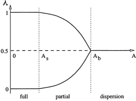
a = P = 1, 7 = 0.5, L — 5 and 0 = 1. Hence, using expressions (42) and (45), the two critical values for the immobile factor are given by A s = 3.5556 < A^ = 4.25. Therefore, we have complete agglomeration if A < 3.5556, dispersion if A > 4.25 and partial agglomeration if 3.5556 < A < 4.25.

Figures 1, 2 and 3 illustrate the three fundamental types of spatial equilibria when

A = 3, A = 3.8 and ^4 = 5 respectively (compare with Figure 5 in Puga [15]). As one can see, when A < A 8y only full agglomeration is a stable equilibrium (the grayed circles in Figure 1) while the symmetric equilibrium is unstable (the empty circle). As A increases to 3.8 (hence A 8 < A < Af,), two partially agglomerated stable interior equilibria appear (grayed circles in Figure 2) while the symmetric equilibrium remains unstable (empty circle). Finally, when A = 5 > A\, gets large, the only stable equilibrium is given by the symmetric dispersed one (the grayed circle in Figure 3).

Figure 4 illustrates a typical bifurcation diagram in our inconditional autarky scenario. As usual, bold solid lines correspond to stable equilibria while bold broken lines correspond to unstable ones. As one can see, there are no catastrophic transitions and the evolution of the spatial equilibria is smooth.

4. Conclusions

As we have shown in this paper, the question of which goods are available where matters in shaping the space-economy. When particular goods are only available in particular locations, the equilibrium configurations can be significantly different from those obtained when everything is available everywhere. In this paper, we have focused

Figure 4: Smooth transitions of equilibria under autarky

on the extreme case of regional autarky in which all goods are only available locally. Although this assumption is not likely to hold for most of todays manufacturing industries, it remains suited either to historical applications, or to the analysis of the spatial distribution of non-tradeables or to the analysis of regional imbalances in developing countries with poor transport infrastructures. Our setting allows for a large range of possible equilibrium configurations, including stable partial agglomeration of activities in the two regions, despite the absence of interregional trade. 9 This clearly shows that trade is neither a necessary nor a sufficient condition fo r agglomeration

to emerge. Taken together, both our paper and those of Puga [15] and Tabuchi and Thisse [16] illustrate that the catastrophic bang-bang behavior of many spatial models disappears when alternative hypotheses concerning the mobility of goods and factors are made. Whereas those models generate partial agglomeration by restricting the mobility of production factors, we have shown here that restricted mobility of outputs can play an analogous role. Therefore both the mobility o f factors and the mobility o f

goods are fundamental in shaping the space-economy and should hence be treated as

9 To the best of our knowledge, the existence of stable partial agglomeration, which is mainly due to the fact that not both goods and factors are simultaneously perfectly mobile, has only been recently shown in a different general equilibrium context by Puga [15] and Tabuchi and Thisse [16].

being equally important.The main result of our model consists in highlighting the fact that when transport costs are high, so that there is no interregional trade, the structure of the spatial economy is determined by the ratio of mobile to immobile factor. Hence/or

a given and fixed total population size, a process o f full or partial agglomeration can

be triggered when the ratio o f mobile to immobile factor rises, even when trade costs

do not decline.We believe this result could partly explain the evolution of economic agglomerations in certain developing countries, especially when we reinterpret the immobile factor as being low-skilled workers whereas the mobile factor corresponds to high-skilled workers. In that case, our results suggest that strong spatial disparities may emerge when an increase in the education level of a growing fraction of the population is not accompanied by a sufficient improvement in infrastructures. More empirical work is called for here.

The main future extension of our approach consists in dropping the admittedly strong assumption of inconditionalautarky and to examine what happens when trade costs take intermediate values. In particular, this case could shed some additional light on the question of whether the larger region will absorb the industry of the smaller one or if there will be regional convergence by redistribution of economic activities as the level of trade costs decrease.

A ppendix

In this technical appendix, we justify the extended demand function as introduced in Section 2 and provide some additional economic interpretations. Consider the implicit consumer problem (Vq) as developed in Section 2, in which the positivity of demands x(i) is implicitly assumed. Each firm indivi­ dually perceivesits extended demand functions

x*(i) = max {0,£*(2)} = [z*(i)]+ , (47) where x*(i) is the solution (2) to the unconstrained problem (Vq). The ex­ tended demand function (47) can be interpreted as the demand function in which the firm adequately, since we are in a monopolistic competition context, neglects the impact of its choices on other firms and vice versa. Hence firm i sets its price p(i) by taking the price aggregate as given and fixed and neglects all possible cross-effects (concerning both prices and quantities) with its com­ petitors. It can be shown that the perceived demand function (47) is generally different from the demand function obtained in the explicit quadratic utility consumer problem, given by

N \ 2 x(i)di ) + xo (Vo e) f N s.t. / p(i)x(i)di + xo = w -f 0o Jo < x (i) > 0 , ¿E[0,iV]

in which the positivity constraints are explicitly introduced and where hence the interdependencies between firms’ prices are taken into account. 10 Roughly

10 This problem is reminiscent of the one arising in a Chamberlinian context with capacity constraints for individual firms. No matter if those constraints are explicitly given or implicitly due to the existence of a profitable capacity (in case of increasing marginal costs), their presence implies that the ‘true’ (or contingent) demand function differs from the actually perceived one. This is, as explained by B6nassy [3], essentially due to the fact that it is

“im plicitly assumed in the construction of the demand curve that each firm can (and will)

speaking, the perceiveddemand function (‘solution’ to {Vq) as given by (47)) abstracts from all cross-effects while the realized(or contingent) demand func­ tion (solution to (‘Pq e)) accounts for those effects. Hence there could a priori be a difference between firm’s perceived and realized demand functions, which would introduce an inconsistency into our model. Nevertheless, as we show now, the two problems yield the same demand functions in our approach, since we use a particular hypothesis. Denote by

C (x,n)

=

J0 x(tfdi ~

(/

rN pN

+ w + (f)o — I p(i)x(i)di + / p(i ) x(i )di

Jo Jo

the lagrangian of the optimization problem ('Pq e). The Karush-Kuhn-Tucker (KKT) conditions are then given by

f N

OL - (p - l ) x { i ) - 7

/

+

rN

p(i) > 0, x(i) > 0 , i € [0, N] and / p(i)x(i)di = 0 (49) Jo

which yields the realized demand functions

r N

Jo \p(j) ~ M(i)]di- (50)

W ~ J ) W +

(N-Now consider the following special assumption, which is of fundamental impor­ tance: if a firm, considering its perceived demand function (47), sets a price

serve any amount of demand forthcoming at any price”. The presence of capacity constraints

creates technical difficulties since, as constraints switch from slack to saturated, kinks appear in the different demands. We face an analogous problem in our approach since the constraints x(i)>0 have the same impact as capacity constraints. Note however that we do not have a profitable capacity in our model since firms operate under constant marginal costs. Hence, we do not have to worry about implicit constraints as demands become ‘large’ but only as demands become ‘small’ (zero in our case).

such that this demand is not strictly positive, the firm will set the lowest possi­ ble price for which this demand is zero. Using firm’s perceived demand function (47) and equating this demand to zero, this price is given by

P{%) = ¡3 + (N - 1)7 + p + ( N - l ) j I P{j)dj• (51) Plugging (51) into the realized demand function (50) yields

* '(i) L ^ a = ^

( " »

- i H N - i h l

M W ) ■

<52)

p(i), the realized demand is zero if the perceived demand is zero (note that the reverse might not be true). Next, use (52) to write

= «(■•)-

0 + (H_

cCiW

and plug this expression into KKT condition (48). Some calculus shows that this condition always holds for all p > 0. Hence it holds for p* = 0.

We can hence conclude as follows. If firm i sets the lowest possible price p(i), given by (51), for which her perceived demand (47) is equal to zero, one can take p* = 0 such that KKT conditions (48) and (49) hold and such that the perceived demand (47) is an optimal solution for the explicit problem (Vq e)-

Hence, the demand functions (47) and (50) coincide in that case.

Finally, we must note that the case in which x*(i) and p*(i) are simulta­ neously equal to zero, is usually a problematic one in optimization since there is no longer a clear relationship between the objective function and the con­ straint. In our problem, this corresponds to the case where the unconstrained maximum of the objective function lies on the boundary of the feasible set (and is hence feasible). Therefore, since our objective function is strictly concave, the consumer problem is always well specified. □

References

[1] P. Bairoch, De Jericho à Mexico - Villes et économie dans l’histoire, Collection Arcades, Paris, Gallimard (1985)

[2] P. Belleflamme, P. Picard, J.-F. Thisse, An economic theory of regional clus­ ters, Journal of Urban Economics 48 (2000), 158-184

[3] J.-P. Bénassy, Monopolistic competition, in: W. Hildenbrand and H. Sonnen- schein (Eds.), Handbook of Mathematical Economics Volume 4, Amsterdam, North Holland (1991), pp. 1997 - 2045

[4] A. Deaton, J. Muellbauer, Economics and consumer behavior, Cambridge, Cambridge University Press (1980)

[5] M. Fajita, P. Krugman, A. Venables, The Spatial Economy - Cities, regions and international trade, Cambridge, MIT Press (1999)

[6] M. Fujita, J.-F. Thisse, Economics of Agglomeration, Cambridge, Cambridge University Press (2002)

[7] V. Ginsburgh, Y. Papageorgiou, J.-F. Thisse, On existence and stability of spatial equilibria and steady-states, Regional Science and Urban Economics 15 (1985), 149-158

[8] M. Greenhut, Spatial pricing in the USA, West Germany and Japan, Economica 48 (1981), 79-86

[9] K. Head, T. Mayer, Non-Europe: The Magnitude and causes of market frag­ mentation in the EU, Weltwirtschaftliches Archiev 136(2) (2000), 285-314

[10] V. Henderson, Z. Shalizi, A. Venables, Geography and development, Journal of Economic Geography 1 (2001), 81-105

[11] P. Krugman, Increasing returns and economic geography, Journal of Political Economy 99 (1991), 483-499

[12] P. Krugman, Pop internationalism, Cambridge, MTT Press (1996)

[13] G. Ottaviano, T. Tabuchi, J.-F. Thisse, Agglomeration and trade revisited, International Economic Review 43(2) (2002), 409 - 435

[14] G. Ottaviano, J.-F. Thisse, On economic geography in economic theory: in­ creasing returns and pecuniary externalities, Journal of Economic Geography 1 (2001), 153-179

[15] D. Puga, The rise and fall of regional inequalities, European Economic Review 43(1999), 3 0 3 -3 3 4

[16] T. Tabuchi, J.-F. Thisse, Labor mobility and economic geography, Journal of Development Economics 69(1) (2002), 155-177

[17] T. Tabuchi, J.-F. Thisse, Regional specialization and transport costs, CEPR Working Paper 3542 (2002)

[18] K. Wong, International trade in goods and factor mobility, Cambridge, MIT Press (1995)