HAL Id: inria-00490195
https://hal.inria.fr/inria-00490195v2
Submitted on 30 Aug 2010
HAL is a multi-disciplinary open access
archive for the deposit and dissemination of
sci-entific research documents, whether they are
pub-lished or not. The documents may come from
teaching and research institutions in France or
abroad, or from public or private research centers.
L’archive ouverte pluridisciplinaire HAL, est
destinée au dépôt et à la diffusion de documents
scientifiques de niveau recherche, publiés ou non,
émanant des établissements d’enseignement et de
recherche français ou étrangers, des laboratoires
publics ou privés.
Reconstructing Social Interactions Using an unreliable
Wireless Sensor Network
Adrien Friggeri, Guillaume Chelius, Eric Fleury, Antoine Fraboulet, France
Mentré, Jean-Christophe Lucet
To cite this version:
Adrien Friggeri, Guillaume Chelius, Eric Fleury, Antoine Fraboulet, France Mentré, et al..
Recon-structing Social Interactions Using an unreliable Wireless Sensor Network. Computer
Communica-tions, Elsevier, 2011, 34 (5), pp.609–618. �10.1016/j.comcom.2010.06.005�. �inria-00490195v2�
Reconstructing Social Interactions Using an unreliable Wireless Sensor
Network
A. Friggeria,∗, G. Cheliusb, E. Fleurya, A. Frabouletd, F. Mentr´ee, J.C. Lucetc
aLIP UMR 5668/ENS de Lyon, DNET/INRIA, Universit´e de Lyon
bDNET/INRIA, LIP UMR 5668/ENS de Lyon, Universit´e de Lyon
cHˆopital Bichat - Claude Bernard, AP-HP, Universit´e Paris-Diderot - Paris VII, Paris
dCITI/INSA de Lyon, AMAZONES/INRIA, Universit´e de Lyon
eUMR 738 INSERM, Universit´e Paris Diderot
Abstract
In the very active field of complex networks, research advances have largely been stimulated by the availability of empirical data and the increase in computational power needed for their analysis. These works have led to the identification of similarities in the structures of such networks arising in very different fields, and to the development of a body of knowledge, tools and methods for their study.
While many interesting questions remain open on the subject of static networks, challenging issues arise from the study of dynamic networks. In particular, the measurement, analysis and modeling of social interactions are first class concerns.
In this article, we address the challenges of capturing physical proximity and social interaction by means of a wireless network. In particular, as a concrete case study, we exhibit the deployment of a wireless sensor network applied to the measurement of Health Care Workers’ exposure to tuberculosis infected patients in a service unit of the Bichat-Claude Bernard hospital in Paris, France. This network has continuously monitored the presence of all HCWs in all rooms of the service during a 3 month period.
We both describe the measurement system that was deployed and some early analysis on the measured data. We highlight the bias introduced by the measurement system reliability and provide a reconstruction method which not only leads to a significantly more coherent and realistic dataset but also evidences phe-nomena a priori hidden in the raw data. By this analysis, we suggest that a processing step is required prior to any adequate exploitation of data gathered thanks to a non-fully reliable measurement architecture.
Keywords: complex networks; interaction networks; wireless sensor networks; medical applications
1. Introduction
Complex networks [12] appear in many contexts: sociology, computer networks, biology, medicine, etc. Their study has shown a rapid growth since the end of the 90s when it was revealed [2, 4, 8, 11, 13, 15] that most real-world complex networks
∗Corresponding author: ENS de Lyon, 46 all´ee d’Italie,
69364 Lyon Cedex 07. Tel: +33 472728000
Email addresses: adrien.friggeri@ens-lyon.fr (A. Friggeri), guillaume.chelius@inria.fr (G. Chelius), eric.fleury@inria.fr (E. Fleury),
antoine.fraboulet@insa-lyon.fr (A. Fraboulet), france.mentre@inserm.fr (F. Mentr´e),
jean-christophe.lucet@bch.ap-hop-paris.fr (J.C. Lucet)
offer common non-trivial properties. This obser-vation has generated a substantial amount of at-tention during the last decade. While a large part of these works have dealt with static networks, a growing area of research is focused on the dynamic aspects of those networks. The introduction of the temporal dimension is motivated by the fact that most real-world complex networks bear an intrin-sic evolution whose analysis and modeling is fun-damental to the understanding of the underlying phenomenon.
In numerous fields of study, be it epidemiology, sociology or even the study of computer networks such as Delay Tolerant Networks, the central rela-tional concept is the social interaction or the
phys-ical proximity. Getting a grasp of these relation-ships is a complex task which is generally fulfilled through audits and interviews, two human-centric approaches. As in the first case, an experimenter monitors and reports the observable interactions whereas in the second one data is compiled thanks to the imperfect memory of the subject, it is obvi-ous that both methods not only suffer from a lack of exhaustivity but also deliver data which reliability heavily depends on human factors. These two mea-surement properties, lack of reliability and lack of exhaustivity, lead to severe limitations in the above-mentioned fields of study.
More recently, with the advances in pervasive networks, wireless devices have offered a new and promising opportunity to gather data on social in-teractions and physical proximity. As a an exam-ple, if phone calls are construed as instances of social interactions, phone records owned by tele-com tele-companies represent precious sets of data to
be analyzed. Surprisingly, not only the
commu-nication but the mere ability to communicate can
be interpreted in term of physical proximity. In
the context or wireless technologies, a communi-cation between two devices is only feasible when both are in range. This relation between radio and physical proximity has been used in several exper-iments [1, 6, 10] in order to measure physical in-teractions and proximity through the exchange of radio packets between laptops, cell phones or ded-icated instruments. Thanks to the embedding of communications devices, which allow passive, peri-odic and automatic measurement, this type of de-ployment offers the opportunity to attempt nearly exhaustive measurement campaigns.
Although offering exhaustivity, this measurement method does not provide reliability. Indeed, as the radio medium is pervasive, the relation between ra-dio distance – perceived in term of signal attenua-tion – and physical distance is far from being pre-dictable. It varies in time and space in a pseudo-random way due to physical phenomenon such as fading and shadowing. In consequence, the mea-surements gathered during such deployments are
noisy and must be considered carefully. In
par-ticular, they can not be exploited without being first cleaned and the original interaction informa-tion being reconstructed. This step is fundamental as analyses and evaluations performed on raw mea-surements can lead to results and conclusions that vary drastically from the ones obtained given the real interactions.
Unfortunately, analyses and evaluations are too often based on raw measurements without consid-ering the error induced by the measurement sys-tem [10] itself. We assess that this methodological shortcut takes root in an over-confidence in comput-ing devices. The assumption that a measurement is not only exhaustive but also reliable due to its nature of computer-gathered data reveals an utter misconception of the measurement apparatus’ lim-its. For the sake of analyses validity, the challenge is thus to process unreliable data using an estimate of the system induced error in order to acquire an accurate picture of the original interactions.
In this paper, we address this issue through a case study, the deployment of a Wireless Sensor Net-work (WSN) to measure in situ interactions within a medical context. This project was motivated by the study of the Health Care Workers (HCWs) ex-posure to tuberculosis in their work environment, as described in Section 3. Sections 4 and 5 present the WSN that was set up to record the presence of HCWs within patient rooms in a specific ser-vice care unit of the Bichat Hospital (Paris France). An important characteristic of this measurement campaign is its exhaustivity: it was performed in a closed environment, over a closed population and during a long and continuous period of time. That is, the presence of all HCWs of the unit was monitored, every 5 seconds, in all patient rooms of the unit, 24 hours a day, 7 days a week, during a three month period. It represents both a huge and unique data set describing a complex dynamic in-teraction network. After describing the raw data that were gathered during the deployment in Sec-tion 6, we emphasize on the bias introduced by the measurement system in Section 7 and show that the versatility of the radio medium leads to noisy and unreliable data. We present in Section 8 a method to reconstruct a presence signal using the available
data and describe the results in Section 9. We
finally conclude and present future works in Sec-tion 10.
2. Contributions
In our opinion, this article presents several con-tributions in the field of physical proximity mea-surement using wireless devices:
• it describes a WSN deployment for physical proximity measurement performed in a closed
environment, over a closed population and during a long and continuous period of time; • it assesses, through an analysis of the raw data, the unreliability of this measurement process; • it investigates methods to quantify the
mea-surement’s error;
• it proposes a method to eliminate false posi-tives and false negaposi-tives in the measured data and to recover the original interaction informa-tion.
3. The TubExpo project
This work was motivated by the AFFSET TubExpo project. This project aims at evaluating the exposure of health care workers to tuberculosis in their work environment.
3.1. The health care context: Tuberculosis
Despite the progresses in treatment and preven-tion, tuberculosis remains a disease in expansion and represents the third cause of death by infectious pathologies in the world. Emerging countries are the most affected, as the VIH epidemic participates to the tuberculosis amplification. In France, the impact of tuberculosis is globally decreasing (9.2 cases for 100000 inhabitants in France) but with large regional disparities. The french situation is paradoxical, with a hygiene level of a developed country but a strong and increasing tuberculosis
incidence among the migrating populations. For
this reason, the french superior council for public hygiene (CSHPF) has recently recommended the launch of studies about the tuberculosis infection and its transmission factors [7].
In the health care context, if the transmis-sion between patients has been largely documented and is globally controlled, the health care workers (HCWs) exposure remains obscure. HCWs taking care of tuberculosis-infected patients are particu-larly exposed to the disease, and, if infected, may become important transmission vectors as they ex-pose both colleagues and patients to the risk of in-fection. In October 2003, six cases of HCW tuber-culosis infection were reported in five hospitals of Paris [5].
Data on the tuberculosis transmission has gen-erally been acquired in a social community con-text. Individual factors associated to the contam-ination of HCWs in their work environment are
not precisely known [14]. Knowledge acquisition
on the transmissibility of the tuberculosis bacilli in the hospital environment is limited by two fac-tors: individual contamination evaluation and ex-posure measurement. The evaluation of these two factors is complicated as they are impacted by
sev-eral sub-factors. For the exposure measurement,
several parameters must be considered: the tuber-culosis bacilli concentration in the environing air, the intensity and frequency of contacts between in-fected patients and HCWs and, finally, the preven-tion methods used to restrain the transmission. 3.2. Visit Measurement: methods
Among these various parameters, the TubExpo project focuses especially on the evaluation of both contacts intensity and frequency between tubercu-losis infected patients and HCWs inside the Service of Infectious and Tropical Diseases (SMIT) of the Bichat-Claude Bernard hospital in Paris, France.
In order to measure the exposure of HCWs to the tuberculosis bacilli, the time spent by the HCWs in each patient room of the unit was monitored during a three months period. As individuals infected or suspected to be infected by tuberculosis are subject to strong isolation rules, we made the hypothesis that the exposure area was limited to their rooms. Obviously, a first limit of the measurement validity is the respect of these isolation rules by the infected patients.
Two different methods were envisaged in order to measure the HCWs presence in patient rooms: the first one is based on manual audits whereas the sec-ond makes use of a wireless sensor network (WSN). 3.2.1. Method 1: Audits
Performing audits is a classical method to gather data on social interactions or work habits, espe-cially in a health care context. Given the human nature of such a measurement, there is no false pos-itive as a visit is never recorded if it did not actually occured. Moreover, this method does not involve any technical aspect and is simple to deploy. How-ever, as a manual recording, this approach is partial because it does not offer a continuous observation. The experimenter has to be present in the unit for the visit to be recorded. As an example, no audit was performed during the night. It is also subject to observations and interpretations: simultaneous visits in different rooms can hardly be handled by a single experimenter. Finally, it is time and human resource consuming.
0 5 10 15 20 25 30 35 40 45 50 0 200 400 600 800 1000 1200 audits duration (seconds)
Figure 1: Cumulative distribution of audit durations.
In our case, 48 visits were manually recorded by an experimenter who recorded the relevant room and HCW id, the time of arrival and the dura-tion of each visit. The average duradura-tion of a visit was of 3min 26s, the shortest 10s and the longest 18min. The distribution of durations corresponding to these audits is given in Figure 1.
Obviously, the knowledge of 48 visits over the course of the three months long experiment does not provide any relevant information per se. However, having access to a frame of reference for attested visits can be insightful when correlated with other data, as we will show in Section 7.
3.2.2. Method 2: WSN
In order to continuously and exhaustively mon-itor the presence of HCWs in patient rooms, the second method we used was to deploy a wireless sensor network in the unit of the hospital. This WSN consisted of devices placed in patient rooms and devices handled by the HCWs. Compared to audits, this method offers exhaustivity: it is oper-ating 24 hours a day, 7 days a week, independently of the presence of an experimenter. However, con-trarily to what could be primarily thought, its reli-ability is subject to many factors and the resulting data should not be considered as a perfect image of the interactions reality. As an example, a first error factor, but not the only one, is the human factor and the acceptance of the deployment by the HCWs. Obviously, measurements can not occur if HCWs forget or refuse to handle their sensor
de-vice. It is worth noting that within the context
of the TubExpo project, only one of the unit’s 63 HCWs refused to be enrolled in the experiment and that all rooms were equipped.
4. A WSN for presence detection
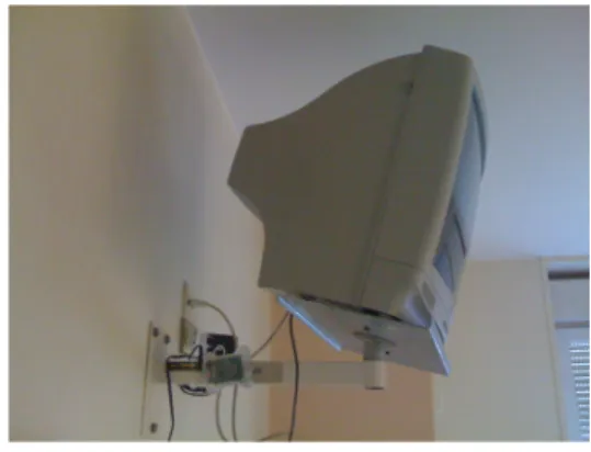
In this deployment, each room of the SMIT unit in the Bichat-Claude Bernard hospital (Paris, France) was equipped with a sensor node whose task was to continuously listen to the radio medium. More precisely, these fixed sensor nodes were placed at a 2m height, under the TV, and plugged to the
power line (Figure 2). They were thus provided
with an unlimited energy resource.
Figure 2: Location of a fixed sensor node in a patient room. In parallel, each HCW was given an autonomous sensor node they had to carry during their presence in the unit. These mobile sensor nodes were pro-grammed to periodically transmit a radio packet
containing their identity. They were under the
HCWs responsibility without the possibility to re-fill their battery during the whole deployment du-ration. This induced strong energy constraints on their functioning.
Contrarily to previous interactions measurement applications [1, 6, 10], we chose to deploy an asym-metric network where only the fixed sensor nodes, i.e. the ones installed in the patient rooms, were re-ceiving packets and recording interactions. Briefly, we can advance three main reasons to justify this choice:
• simplicity: in such an asymmetric network, a sensor node does not need to switch between transmission and reception modes, therefore avoiding synchronization issues among oth-ers and largely simplifying the sensor node firmwares.
• energy consumption: as the fixed nodes were not energy constrained, they could perma-nently stay in reception mode and no activity scheduling or duty-cycling policy was required.
On the contrary, HCW-carried sensor nodes were strongly energy constrained and their ra-dio I/O operations had to be limited to the minimum.
• privacy respect: as we were only interested in the presence of HCWs in patient rooms, we did not need to record the proximity of HCWs between each other. Doing so would not only have required additional privacy respect proce-dures but also a stronger defense of the project in front of privacy & work protection commit-tees.
Fixed sensor node Off!duty HCW mobile sensor nodes
32 30 12 10 9 8 6 4 5 3 2 1 35 34 & 34bis 33 31 29 28 27 26 25 & 25bis 24 20 19 23 22 21 17 16 15 14 11 & 11bis
Figure 3: A map of the Service of Infectious and Tropi-cal Diseases (SMIT) at the Bichat-Claude Bernard hospital (Paris, France) together with the fixed sensor node locations (red circles).
The deployed sensor network is depicted in Fig-ure 3. The SMIT is composed of 32 patient rooms which are split in two T shaped aisles. The SMIT owns 63 HCWs, all but one carrying a mobile sen-sor node. The network was thus composed of 94 sensor nodes that have operated continuously dur-ing the three months experiment period. To our knowledge this experiment is the first proximity in-teraction study performed over a complete closed population during a so long continuous period of time: all but one HCWs of the unit carried a sen-sor node, each room of the unit was monitored and HCWs were not supposed to leave the unit during their duty.
5. Hardware and protocol details 5.1. Hardware
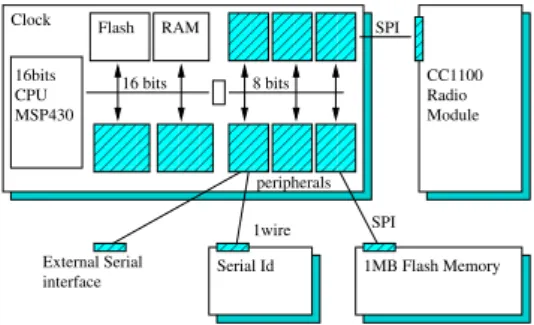
The deployment was conducted using WSN430 sensor nodes [9]. Their internal architecture is clas-sical and similar to commercially-available sensor
Serial Id 1wire
Flash RAM
16bits 16 bits 8 bits
peripherals Clock 1MB Flash Memory SPI SPI CC1100 Radio Module CPU MSP430 External Serial interface 00 00 00 11 11 11 00 00 00 11 11 11 00 00 00 11 11 11 00 00 00 00 11 11 11 11 00 00 00 00 11 11 11 11 00 00 00 00 11 11 11 11 00 00 11 11 000 000 000 111 111 111 0 0 0 1 1 1 000 000 000 111 111 111 00 00 11 11 00 00 11 11
Figure 4: A simplistic schematic of a WSN430 node.
nodes. Very basically, they are composed of a
micro-controller, a RF chipset, a flash memory, sev-eral crystals, a lithium-ion battery and an on-board PCB antenna (Figure 4). The micro-controller be-longs to the TI MSP430 family. The RF chipset is a TI CC1100 operating at the 868MHz frequency, with a 2-FSK modulation and a 119Kbps baud-rate. The flash memory storage size is 1Mb. Figure 5 il-lustrates a WSN430 node in its plastic packaging.
Figure 5: A WSN430 sensor node.
5.2. Neighbor discovery protocol
Proximity detection was achieved through the periodical emission of Hello packets. This strat-egy has the merit of simplicity and has been used
in other deployments [3]. It is quite similar to
the Bluetooth base-band layer inquiry method used in [10]. However, contrarily to these previous works, we did not implement any random access scheme to the radio medium but rather set up a deterministic TDMA scheme. Under this scheme, the timeline is divided in windows of W seconds and each
win-dow is split in 100W time slots. Each mobile sensor
node owns a time slot it uses to transmit its Hello packet. Synchronization of the mobile nodes was performed at the experiment startup.
As described in [3], the performance of this very simple neighbor discovery protocol, and thus the
quality of the proximity detection, largely relies on the dimensioning of the protocol parameters. In our case, the parameters are the window duration W , the transmission power T and reception level
thresholds {Ri}. The parameters values were
cho-sen after a pre-deployment dimensioning phase dur-ing which different scenarios were explored and sev-eral parameter value sets experimented. The final values are given in Section 5.4. We also based our choices on the HCWs recommendations and their work habits observation. For example, it appeared quickly that most of the HCW presences in patient rooms were brief, around a few minutes, requiring a short W duration to ensure some reliability in the discovery process. As a comparison, the 120s pe-riod used in [10] is far too long to detect most of the HCWs presences in patient rooms.
5.3. Versatility of the radio medium
Three other major observations were made dur-ing this pre-deployment dimensiondur-ing phase:
• the system suffers an important packet loss, even at short ranges;
• the relation between radio signal attenuation and physical distance is weak;
• the radio signal attenuation is not predictable and can largely vary.
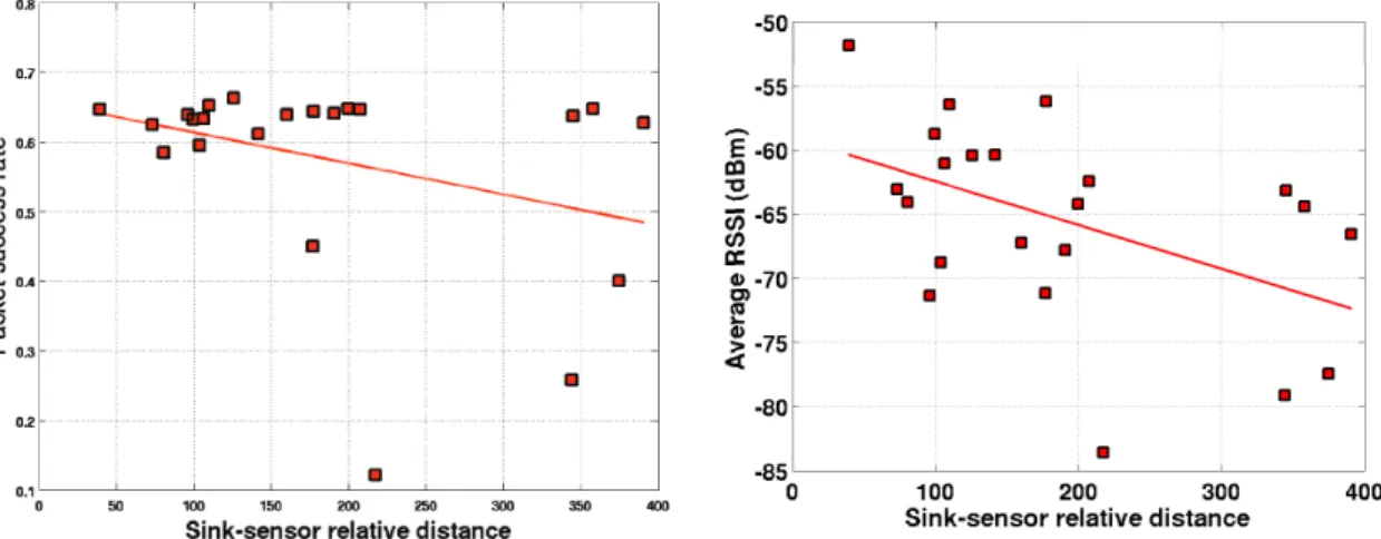
Figure 6 illustrates the two first claims. It depicts the relation between distance and the Received Sig-nal Strength (RSSI) and the packet loss that the system experienced during a pre-deployment exper-iment involving 22 sensor nodes. The third claim can be observed in Figure 7 where the RSSI and its standard variation is plot against time for three ra-dio links. From all these results, it appears clearly that the RSSI value is not stable in time nor in space. These variations are due to well-known fad-ing and shadowfad-ing effects but also to the human body which offers strong attenuation properties. For example, depending on the HCW attitude and their position in the room, RSSI variations up to 20dBm can be observed. Under these conditions, it is very tricky to differentiate a contact with a HCW in front but outside a room from a contact with a HCW inside a room but with their body between the mobile device and the fixed one.
The impact of the packet loss and the RSSI vari-ability on the measurement relivari-ability is obvious: it leads to false-negatives, in-room presences that
are not recorded, but also false-positives, as when a HCW is facing the fixed sensor node from outside the room. From this pre-deployment phase, we can already draw some conclusions:
• a correct dimensioning of the neighbour proto-col is required to limit the measurement system error;
• the measurements collected by such a deploy-ment are partially erroneous and should not serve for application analysis or evaluation without being somehow corrected.
5.4. Protocol dimensioning
RSSI level 4 3 2 1
dBm ≥ −60 ≥ −65 ≥ −70 ≥ −75
Table 1: RSSI Thresholds.
W Transmission power
5s 0dBm
Table 2: Proximity detection parameters.
The high system loss rate combined to the usually brief presence of HCWs in rooms required the use of a short W value to ensure reliability in the prox-imity detection system. Moreover, due to the high variations in the received signal strength, the prox-imity detection could not be performed using a sin-gle RSSI threshold only. Instead, we had to record more information on the received signal strength as-sociated to each contact, i.e. each received packet. Given the sensor node memory constraints – their storage size is 1M b only – and the deployment dura-tion, recording the exact reception strength was not an option. Instead, we defined four reception levels, corresponding to four signal strength intervals, and recorded each contact together with its reception level. The protocol parameters and the reception levels that were finally used in the deployment are given in Tables 1 and 2.
6. Raw Data – Observations
The resulting data consists of 16, 066, 096 con-tacts over a period of 98 days between 56 HCWs – 6 of the mobile sensors failed to report any data – and 32 rooms. A contact c = (t, m, f, r) indicates that fixed sensor f received a signal from mobile
Figure 6: Average RSSI (left) and packet delivery ratio (right) versus sink-sensor relative distance.
Figure 7: RSSI (left) and RSSI standard deviation (right) variations over time for three radio links.
sensor m with a RSSI r ∈ [1, 4], 1 being the weak-est and 4 being the strongweak-est, at time t.
As the measurement of contacts was made dis-cretely, we extend the notion of contact to the one of visit v = (t, d, m, f, r) where d is the maximal duration of the contact. In other words, if a signal from m is received by f with RSSI ≥ r every 5 sec-onds between t and t + d, we consider that there is a visit of RSSI r during all that period.
Looking at the data, we note that the number of contacts per fixed sensor is heterogeneous
(Fig-ure 8). The apparent absence of data for some
rooms is due to the fact that their are no rooms numbered 7, 13 and 18 in the service, as shown on Figure 3. By observing the distribution of number of contacts, we were able to isolate rooms 14 and 17 from the other rooms for having an abnormally
high number of contacts. It appeared that these room are next to the room where unused mobile sensors were stocked at night (Figure 3) and there-fore were continuously receiving radio packets from those sensors even though no HCW was present in the room.
Out of the 30 remaining rooms (Figure 8), the number of contacts span from less than 100, 000 to more than 1, 000, 000. Moreover, when decompos-ing this number by RSSI level, it is noticeable that there is no global trend : room 8 has about 100, 000 contacts of RSSI 4 (more than 10% of its contacts) whereas room 6 has less than 5, 000 (less than 5% of its contacts).
The distribution of contacts per mobile sensor (Figure 8) is heterogeneous as well. 4 sensors have been seen less than 1, 000 times whereas all 52
1 10 100 1000 10000 100000 1e+06 rooms contacts 1000 10000 100000 1e+06 1e+07 5 10 15 20 25 30 35 contacts rooms rssi = 1 rssi = 2 rssi = 3 rssi = 4 1 10 100 10 100 1000 10000 100000 1e+06 mobile sensors contacts 10 100 1000 10000 100000 1e+06 10 20 30 40 50 60 contacts mobile sensors rssi = 1 rssi = 2 rssi = 3 rssi = 4 1 10 100 100 1000 10000 100000 days contacts 100 1000 10000 100000 1e+06 10 20 30 40 50 60 70 80 90 contacts day rssi = 1 rssi = 2 rssi = 3 rssi = 4
Figure 8: Number of contacts received by fixed sensors, mobile sensors, deployment day and the reversed cumulative distribu-tions of level 4 contacts.
ers were seen at least 10, 000 times (taking into account all RSSIs). These differences can be ex-plained by the intrinsic heterogeneity of HCWs, as nurses do not have the same behaviour as doctors, interns or social assistants.
The distribution of contacts per day of deploy-ment (Figure 8) displays a heterogeneous behav-ior at a daily level although weekly trends are evi-denced with a lower activity towards the end of the week. Moreover, activity varies from one week to another, e.g.. weeks 7 & 8 (days 49 through 62) have a low activity whereas week 2 (days 7 through 14) has a higher activity. It is interesting to notice that the former two weeks were official holidays in
France, probably with less HCWs present in the service.
In the rest of the article, we focus on a subset of the data consisting of the interactions between all HCWs and 63 patients monitored for being poten-tially infected by tuberculosis.
7. Error model 7.1. False negatives
Packet loss. We call intercontact the duration be-tween two consecutive contacts bebe-tween a same cou-ple (fixed, mobile) of sensors. This duration
1e-06 1e-05 0.0001 0.001 0.01 0.1 1 1 10 100 1000 1e-06 1e-05 0.0001 0.001 0.01 0.1 1 1 10 100 1000 10000 100000 1e+06 1e+07
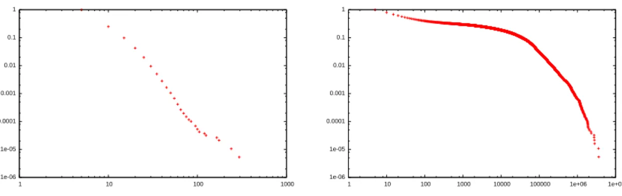
Figure 9: Distributions of visits durations (left) and intercontacts (right).
sents the time during which a HCW is absent from a room before re-entering.
By observing the distributions of both visits and intercontacts durations (Figure 9), we notice that 90% of all visits last at most 10s and that moreover 30% of intercontacts last less than 15s. Those two observations are blatantly erroneous and can be ex-plained by the volatility of the radio medium. Loss of packets induces false negatives in the measure-ment.
Assuming a uniform and stationary packet loss, we propose a method to evaluate the probability p of receiving a packet based on the intercontacts distribution and further confirmed by the audits.
Probability of measuring a contact. It is legitimate to suppose that there exists a minimal intercontact duration which corresponds to the fact that a HCW does not exit a room only to re-enter a few seconds
later. We suppose that this duration is at least
equal to 20s.
As a consequence, we can consider that intercon-tacts of less than 20s are due to a packet loss, and thus the probability of measuring an intercontact of 5k seconds is exactly the probability of losing k consecutive packets. Hence, assuming a uniform
and stationary loss, (1 − p)k. Using the measured
data, we estimate p ∼ 0.13.
Validation using the audits. By comparing the au-dits and the data obtained during the same period, we can evaluate p as being the fraction of measured presence per effective presence. We estimate by this method that p ∼ 0.145 which is coherent with the value obtained by the observation of short intercon-tacts.
7.2. False positives
The existence of a contact does not guarantee an actual presence in the room. Due to the nature of the radio medium, the signal from a HCW walking in front of an opened door or in an adjacent room might be received with a higher strength than that of a HCW in the room but turning its back to the fixed sensor. Although the probability of having a false positive might be small, it is important to keep in mind that because of the great number of contacts, a lot of false positives might arise. We assume that the probability of measuring a false positive is uniform and stationary, hence the prob-ability of having k consecutive contacts decreases exponentially with k.
8. Reconstruction method
Due to these observations, reconstructing the original signal is a necessity, as the measured data does not represent actual social interactions. We thus propose the following reconstruction protocal, illustrated in Figure 10:
• reveal false negatives:
– determine the minimal intercontact
dura-tion di;
– aggregate successive contacts separated
by at most di seconds;
• delete false positives:
– determine the minimal visit duration dv
1e-09 1e-08 1e-07 1e-06 1e-05 0.0001 0.001 0.01 0.1 1 10 100 1000 10000 100000 1e+06 1e-08 1e-07 1e-06 1e-05 0.0001 0.001 0.01 0.1 1 10 100 1000 10000 100000 1e+06 1e-10 1e-09 1e-08 1e-07 1e-06 1e-05 0.0001 0.001 0.01 0.1 1 10 100 1000 10000 100000 1e+06 1e+07 1e-09 1e-08 1e-07 1e-06 1e-05 0.0001 0.001 0.01 0.1 1 10 100 1000 10000 100000 1e+06 1e-09 1e-08 1e-07 1e-06 1e-05 0.0001 0.001 0.01 0.1 1 10 100 1000 10000 100000 1e+06 1e-10 1e-09 1e-08 1e-07 1e-06 1e-05 0.0001 0.001 0.01 0.1 1 10 100 1000 10000 100000 1e+06 1e-10 1e-09 1e-08 1e-07 1e-06 1e-05 0.0001 0.001 0.01 0.1 1 10 100 1000 10000 100000 1e+06 1e+07 1e-09 1e-08 1e-07 1e-06 1e-05 0.0001 0.001 0.01 0.1 1 10 100 1000 10000 100000 1e+06 1e-09 1e-08 1e-07 1e-06 1e-05 0.0001 0.001 0.01 0.1 1 10 100 1000 10000 100000 1e+06 1e-10 1e-09 1e-08 1e-07 1e-06 1e-05 0.0001 0.001 0.01 0.1 1 10 100 1000 10000 100000 1e+06 1e+07 1e-09 1e-08 1e-07 1e-06 1e-05 0.0001 0.001 0.01 0.1 1 10 100 1000 10000 100000 1e+06 1e-10 1e-09 1e-08 1e-07 1e-06 1e-05 0.0001 0.001 0.01 0.1 1 10 100 1000 10000 100000 1e+06 1e+07
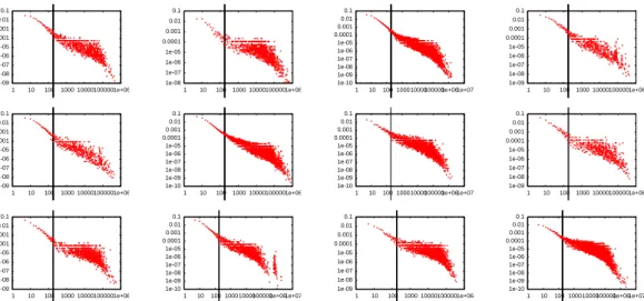
Figure 11: Right derivative of the reversed cumulative distribution of intercontacts durations in different rooms. The vertical line indicates 180s.
Figure 10: Illustration of the reconstruction protocol.
8.1. Minimal intercontact duration
As explained before, short intercontacts are solely
a consequence of the packet loss. By observing
the distributions of intercontacts durations for each room, we note on Figure 11 a change of behavior (inflection of the derivative of the reversed cumula-tive distribution function) around 180s. The change represents the fact that longer intercontacts are not only due to packet loss but also to the HCW be-havior and thus to actual intercontacts. Hence, we
consider di= 180.
8.2. Minimal visit duration
We first aggregate all contacts separated by at
most di seconds and plot, for each duration d and
each room r the fraction of the total presence du-ration in room r due to visits of dudu-ration d as a function of the proportion of visits of duration d in this room. This represents the relationship between contributions in terms of duration and number of visits of each duration. On Figure 12 we observe that the visits of 5 seconds, highlighted on the fig-ure and contained in the right bow area, display
0.0001 0.001 0.01 0.1 1 0.0001 0.001 0.01 0.1 1 "5" "10"
Figure 12: Contributions of visits, per room and duration, to the total of visits and durations.
a totally different contribution than that of other durations, and we conclude that the minimal visit duration is at least 10 seconds. Given that there is no clear separation between the contributions of
visits of more than 10s, we assume dv= 10.
9. Results 9.1. Intercontacts
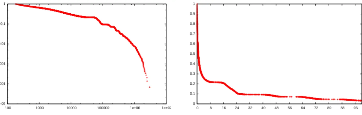
After reconstruction, we obtain the distribution of intercontacts given in Figure 13. Its apparent irregularity, which was not present beforehand, is explained by the work schedule of HCW and in par-ticular by the fact that the maximum work (respec-tively rest) period per day is around 8h (resp. 16h). Thus, for example, there are very few intercontacts which duration is more than 8h and less than 16h.
1e-05 0.0001 0.001 0.01 0.1 1 100 1000 10000 100000 1e+06 1e+07 0 0.1 0.2 0.3 0.4 0.5 0.6 0.7 0.8 0.9 1 0 8 16 24 32 40 48 56 64 72 80 88 96
Figure 13: Distribution of intercontacts durations after reconstruction (left) and zoom on the first 100 hours (right).
1e-05 0.0001 0.001 0.01 0.1 1 10 100 1000 10000 100000 1e+06 outliers
Figure 14: Distribution of visits durations after reconstruc-tion.
This observation reinforces the idea that the re-construction method is correct, as it brings out ret-rospectively a real behavior which was not explicit in the original distribution and which is not due to a reconstruction bias.
9.2. Visits
The distribution of visits durations (Figure 14) clearly highlights the presence of outliers, i.e. vis-its which durations are abnormally high. These 23 outliers are divided as follow: 19 visits of doctors in room 19 (next to a room used by doctors for com-puter work), 3 visits of a nurse in room 14 (next to the room where sensors were stocked when not used) and one visit of a nurse in room 8 (adjacent to the room where HCW stayed while not in the pa-tient rooms). Given that those outliers’ existence can be explained by the service’s topography or by the negligence of a HCW (forgetting a blouse in a room, for example), we consider that they are not a reconstruction error and propose their deletion from the dataset.
9.3. Some statistics
In order to exhibit the differences induced by the reconstruction we present in Table 3 a compari-son of several statistics on the number and dura-tions of visits to selected patients before and af-ter reconstructing the presence signal. It makes no doubt that any further exploitation of the HCW vis-its data will be altered depending on wether they would have been based on the raw measures or the reconstructed interactions.
10. Conclusion
The data collected within the framework of the TubExpo project is huge and unique in nature, con-sisting in the record of the HCWs presence in all patient rooms of the SMIT unit, 24 hours a day, 7 days a week, during a three months period and on a 5s basis. Using this data set, we have highlighted the bias introduced by the measurement system, mainly caused by the radio medium versatility, and we have argued that this bias can lead to major miss-interpretation of the data and/or wrong model behaviors. In order to correctly exploit the data and recover from measurement errors, we have de-vised a method that can be used to reconstruct the original interactions information and which uncov-ers phenomena which were not visible on the raw data.
Now that the issue of measurement reliability has been clearly identified, many points remain as fu-ture extensions of this work. Alternate reconstruc-tion algorithms can be investigated and in partic-ular, an individual analysis leading to a specializa-tion of the reconstrucspecializa-tion parameters to the dif-ferent sensor nodes appears as a promising
Patient Nb of visits shortest (s) longest (s) average duration (s) std dev median (s) 25 1089 75 5 10 30 640 5.50 140.13 2.02 151.38 5 100 26 3860 368 5 10 40 3850 6.74 283.65 3.79 421.94 5 135 27 1849 169 5 10 60 2155 7.59 233.58 5.67 329.85 5 115 28 1148 120 5 10 50 2415 6.96 309.25 4.52 411.68 5 170 29 7639 684 5 10 55 3160 7.26 277.76 4.73 327.60 5 175 30 11157 1151 5 10 60 3600 7.47 252.72 4.92 370.92 5 125 31 1911 143 5 10 60 2175 6.94 162.55 5.44 251.00 5 95 32 2105 166 5 10 30 985 5.54 126.96 2.16 155.41 5 75 33 5392 441 5 10 35 1255 5.79 156.35 2.60 184.00 5 100 34 3231 365 5 10 80 1600 7.79 201.03 6.69 225.85 5 135
Table 3: Various statistics before (left) and after (right) reconstruction for a subset of the patients
towards analyzing the TubExpo data set with re-spect to additional health care information related to the patients that was collected during the exper-imentation. We have to address more sophisticated models both from the clinical/health care perspec-tive, e.g. epidemic models, health care strategies or public health policies, and from the network analy-sis perspective in order to answer the fundamental questions that have originally motivated this work.
11. Acknowledgments
This work was supported by a public grant from the French National Agency for Food, Environmental and Occupational Health Safety (ANSES/AFSSET, EST 2007-50)
References
[1] H. Alani, M. Szomsor, C. Cattuto, W. Van den Broeck,
G. Correndo, and A. Barrat. Live social
seman-tics. In 8th International Semantic Web Conference
(ISWC2009), Washington DC, USA, October 2009. [2] R. Albert, H. Jeong, and AL. Barab´asi. The diameter
of the World Wide Web. Nature, 401:130–131, 1999. [3] E. Ben Hamida, G. Chelius, A. Busson, and E. Fleury.
Neighbor discover y in multi-hop wireless networks: evaluation and dimensioning with interference consid-erations. Discrete Mathematics and Theoretical Com-puter Science, 10(2):87–14, 2008.
[4] A.Z. Broder, S.R. Kumar, F. Maghoul, P. Ragha-van, S. Rajagopalan, R. Stata, A. Tomkins, and J. L. Wiener. Graph structure in the web. Computer Net-works, 33, 2000.
[5] A. Carbonne, C. Poirier, G. Antoniotti, C. Burnat, C. Delacourt, C. Orzechowski, P. Astagneau, and E. Bouvet. Investigation of patient contacts of health care workers with infectious tuberculosis: 6 cases in the paris area. The International Journal of Tuberculosis and Lung Disease, 9(8):848–852, 2005.
[6] C. Cattuto, A. Barrat, and W. Van den Broeck. http://www.sociopatterns.org/.
[7] CSHPF. Enquˆete autour d’un cas de
tubercu-lose: recommandations pratiques. Conseil sup´erieur d’hygi`ene publique de France, 2006.
[8] M. Faloutsos, P. Faloutsos, and C. Faloutsos. On power-law relationships of the internet topology. In ACM SIG-COMM, 1999.
[9] A. Fraboulet, G. Chelius, and E. Fleury. Worldsens: de-velopment and prototyping tools for application specific wireless sensors networks. In International Symposium on Information Processing in Sensor Networks (IPSN), Boston, USA, April 2007. ACM.
[10] P. Hui, A. Chaintreau, J. Scott, R. Glass, J. Crowcroft,
and C. Diot. Pocket switched networks and human
mobility in conference environments. In SIGCOMM, Philadelphia, USA, August 2005. ACM.
[11] J. M. Kleinberg, R. Kumar, P. Raghavan, S. Ra-jagopalan, and A. S. Tomkins. The web as a graph:
Measurements, models, and methods. In COCOON,
1999.
[12] R. Kumar and M. Latapy. Theoretical computer science special issue on complex networks – foreword. Theoret-ical Computer Science, 355(1):1–5, April 2006. [13] Mark Newman, Albert-Laszlo Barab´asi, and Duncan J.
Watts. The Structure and Dynamics of Networks.
Princeton University Press, Princeton, USA, 2006. [14] A. Seidler, A. Nienhaus, and R. Diel. Review of
epi-demiological studies on the occupational risk of tuber-culosis in low-incidence areas. Respiration, 72:431–446, 2005.
[15] D. Watts and S. Strogatz. Collective dynamics of ’small-world’ networks. Nature, 393:440–442, June 1998.