HAL Id: hal-00646894
https://hal.archives-ouvertes.fr/hal-00646894v4
Submitted on 16 Apr 2013
HAL is a multi-disciplinary open access
archive for the deposit and dissemination of
sci-entific research documents, whether they are
pub-lished or not. The documents may come from
teaching and research institutions in France or
abroad, or from public or private research centers.
L’archive ouverte pluridisciplinaire HAL, est
destinée au dépôt et à la diffusion de documents
scientifiques de niveau recherche, publiés ou non,
émanant des établissements d’enseignement et de
recherche français ou étrangers, des laboratoires
publics ou privés.
Accuracy of Homology based Approaches for Coverage
Hole Detection in Wireless Sensor Networks
Feng Yan, Philippe Martins, Laurent Decreusefond
To cite this version:
Feng Yan, Philippe Martins, Laurent Decreusefond. Accuracy of Homology based Approaches for
Coverage Hole Detection in Wireless Sensor Networks. ICC 2012, Jun 2012, Ottawa, Canada. pp.497
- 502. �hal-00646894v4�
Accuracy of Homology based Approaches for
Coverage Hole Detection in Wireless Sensor
Networks
Feng Yan, Philippe Martins, Laurent Decreusefond
Network and Computer Science Department TELECOM ParisTech
Paris, France
Email:{fyan, martins, [email protected]}
Abstract—Homology theory provides new and powerful
so-lutions to address the coverage problems in wireless sensor networks (WSNs). They are based on algebraic objects, such as ˇCech complex and Rips complex. ˇCech complex gives accu-rate information about coverage quality but requires a precise knowledge of the relative locations of nodes. This assumption is rather strong and hard to implement in practical deployments. Rips complex provides an approximation of ˇCech complex. It is easier to build and does not require knowledge of nodes location. This simplicity is at the expense of accuracy. Rips complex can not always detect all coverage holes. It is then necessary to evaluate its accuracy. This work proposes to use the area of undiscovered coverage holes per unit of surface as performance criteria. Investigations show that it depends on the ratio of communication and sensing ranges of each sensor. Closed form expressions for lower and upper bounds of the accuracy are also derived. Simulation results are consistent with the proposed analytical lower bound, with a maximum difference of 0.4%. Upper bound performance depends on the ratio of communication and sensing ranges.
I. INTRODUCTION
Wireless sensor networks (WSNs) have attracted a great deal of research attention due to their wide potential applications such as battlefield surveillance, environmental monitoring and intrusion detection. Many of these applications require a reliable detection of specified events. Such requirement can be guaranteed only if the target field monitored by a WSN contains no coverage holes, that is to say regions of the domain not monitored by any sensor. Coverage holes can be formed for many reasons, such as random deployment, energy depletion or destruction of sensors. Consequently, it is essential to detect and localize coverage holes in order to ensure the full operability of a WSN.
There is already an extensive literature about the cover-age problems in WSNs. Several approaches are based on computational geometry with tools such as Voronoi diagram and Delaunay triangulations, to discover coverage holes [1]– [3]. These methods require precise information about sensor locations. This substantially limits their applicability since acquiring accurate location information is either expensive or impractical in many settings. Some other approaches attempt to discover coverage holes by using only relative distances
between neighboring sensors [4], [5]. Similarly, obtaining precise range between neighbor nodes is costly.
More recently, homology is utilized in [6]–[8] to address the coverage problems in WSNs. Ghrist and his collaborators in-troduced a combinatorial object, ˇCech complex (also known as nerve complex), which fully characterizes coverage properties of a WSN (existence and locations of holes). Unfortunately, this object is very difficult to construct as it requires rather precise informations about the relative locations of sensors. Thus, they introduced a more easily computable complex, Rips complex (also known as Vietoris-Rips complex). This complex is constructed with the sole knowledge of the connectivity graph of the network and gives an approximate coverage by simple algebraic calculations. As regards implementation in real WSN, these homology based methods are necessarily centralized, which makes them impractical in large scale sensor networks. Some algorithms have been proposed to implement the above mentioned ideas in a distributed context, see [9]–[11].
As alluded above, Rips complex can not always detect all coverage holes. For instance, in Figure 2, there exists a hole inside the triangle [1, 2, 6] of the ˇCech complex though there is no hole in the same triangle of the Rips complex. It is thus of paramount importance to determine the proportion of missed coverage holes to assess the accuracy of Rips complex based coverage detection. In this paper, it is indicated that such proportion is related to the ratio between communication and sensing ranges of each sensor. In addition, closed form expressions for lower and upper bounds of the proportion are derived. A few papers [12]–[14] provide some results on coverage probability but with a different point of view.
This paper is organized as follows. Section II introduces the network model and the formal definition of triangular holes. Upper and lower bounds of the area of triangular holes per unit of surface for different values of the ratio of communication radius by sensing radius are computed in Section III. Simulation results are compared with theoretical computation in Section IV. Finally, Section V concludes the paper.
II. MODELS AND DEFINITIONS
A brief introduction to the tools used in the paper is given. For further readings, see [8] and references therein. Given a set of points V , a k-simplex is an unordered set [v0, v1, ..., vk]⊆
V where vi6= vj for alli6= j. So a 0-simplex is a vertex, a
1-simplex is an edge and a 2-1-simplex is a triangle with its interior included, see Figure 1. The faces of this k-simplex consist of all (k-1)-simplex of the form [v0, ..., vi−1, vi+1, ..., vk] for
0 ≤ i ≤ k. A simplicial complex is a collection of simplices which is closed with respect to inclusion of faces.
Fig. 1: 0-, 1- and 2-simplex ˇ
Cech complex and Rips complex are two simplicial com-plexes defined as follows [8].
Definition 1 (ˇCech complex). Given a collection of sets U, ˇ
Cech complex of U, ˇC(U), is the abstract simplicial complex whose k-simplices correspond to nonempty intersections of k + 1 distinct elements of U.
Definition 2 (Rips complex). Given a set of points X in Rn
and a fixed radius ǫ, the Rips complex of X , Rǫ(X ), is the
abstract simplicial complex whose k-simplices correspond to unordered (k + 1)-tuples of points in X which are pairwise within Euclidean distance ǫ of each other.
Consider a collection of stationary sensors (also called nodes) deployed randomly in a planar target field. As usual, isotropic radio propagation is assumed. Each sensor monitors a region within a circle of radius Rs and may communicate
with other sensors within a circle of radiusRc. LetV denote
the set of sensor locations in a WSN andS = {sv, v∈ V} the
collection of sensing ranges of these sensors: For a location v, sv = {x ∈ R2 : kx − vk ≤ Rs}. Then, according
to the definition, the ˇCech complex and Rips complex of the WSN, respectively denoted by ˇCRs(V) and RRc(V), can be constructed as follows: [v1,· · · , vk] belongs to ˇCRs(V) whenever ∩kl=1svl 6= ∅ and [v1,· · · , vk] belongs to RRc(V) whenever kvl− vmk ≤ Rc for all1≤ l < m ≤ k.
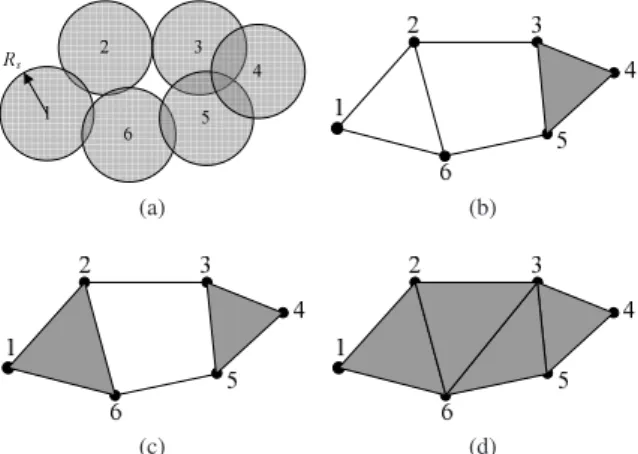
Figure 2 shows a WSN, its ˇCech complex and two Rips complexes for two different values of Rc. Depending on the
ratioRcoverRs, the Rips complex and the ˇCech complex may
be close or rather different. In this example, for Rc = 2Rs,
the Rips complex sees the hole surrounded by [2, 3, 5, 6] as in the ˇCech complex whereas it is missed in the Rips complex for Rc = 2.5Rs. At the same time, the true coverage hole
surrounded by [1, 2, 6] is missed in both Rips complexes. As a consequence of Rips complex definition, a hole in a ˇCech complex not seen in a Rips complex is bounded by a triangle. Based on this observation, a formal definition of ’triangular holes’ is given as follows.
(a) (b)
(c) (d)
Fig. 2: (a) a WSN, (b) ˇCech complex, (c) Rips Complex under Rc = 2Rs, (d) Rips Complex underRc= 2.5Rs
Definition 3 (Triangular hole). For a pair of complexes ˇ
CRs(V) and RRc(V), a triangular hole is an uncovered region
bounded by a triangle which appears in RRc(V) but not in ˇ
CRs(V).
It can easily be seen that there is one triangular hole in the Rips complex in Figure 2(c) and there are three triangular holes in the Rips complex in Figure 2(d). We are interested in the proportion of the area of triangular holes in a target field. Assume sensor nodes are distributed in the planar target field according to a homogeneous Poisson process with intensityλ. Because of homogeneity property, each point in the target field has an equal probability of belonging to a triangular hole. This probability in a homogeneous setting is equal to the proportion of the area of triangular holes. So we only need to compute the probability that any point belongs to a triangular hole.
III. BOUNDS ON PROPORTION OF THE AREA OF TRIANGULAR HOLES
In this section, the conditions under which any point in the target field belongs to a triangular hole are first given. From the discussion in Section II, it is found that the probability that any point belongs to a triangular hole is related to the ratio Rc/Rs. Three different cases are considered for the probability
computation. For each case, the upper and lower bounds of the probability are derived. Let defineγ = Rc/Rs.
A. Preliminary
Lemma 1. For any point in the target field, it belongs to a
triangular hole if the following two conditions are satisfied:
1) the distance between the point and its nearest sensor is
larger than Rs.
2) the point is inside a triangle: the convex hull of three
nodes, two by two less thatRc apart.
Lemma 2. If there exists a point O which belongs to a
triangular hole, thenRs< Rc/
√
3. Furthermore, if l denotes
the distance between O and its closest neighbor, we have Rs< l≤ Rc/
√ 3.
Proof: Rs < l is a direct corollary from Lemma 1. We
only need to prove l ≤ Rc/√3. If point O belongs to a
triangular hole, it must be surrounded by a triangle formed by sensor with pairwise distance less than Rc. Assume it is
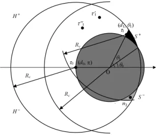
surrounded by a triangleN0N1N2, as in Figure 3. The closest
neighbor of O is not necessarily in the set {N0, N1, N2}. If
l > Rc/√3, then d0 ≥ l > Rc/√3, d1 ≥ l > Rc/√3 and
d2≥ l > Rc/√3. In addition, since ∠N0ON1+ ∠N1ON2+
∠N0ON2 = 2π, there must be one angle no smaller than
2π/3. Assume ∠N0ON2 ≥ 2π/3 and denote it as α. Then
according to the law of cosines,d2
02= d20+d22−2d0d2cos α >
R2
c/3+R2c/3−2/3RcRccos(2π/3) = R2c. Sod02> Rc. Since
N0andN2are neighbors,d02≤ Rc. There is a contradiction.
Therefore l≤ Rc/√3.
Fig. 3: triangular point
A Poisson point process whose intensity is proportional to the Lebesgue measure is stationary in the sense that any translation of its atoms by a fixed vector does not change its law. Thus any point has the same probability to belong to a triangular hole as the origin O. This probability in a homogeneous setting is also equal to the area of triangular holes per unit of surface. We borrow the line of proof from [14] where a similar problem was analyzed.
We consider the probability that the origin O belongs to a triangular hole. Since the length of each edge in the Rips complex must be at most Rc, only the nodes withinRc from
the origin can contribute to the triangle bounding a triangular hole to which the origin belongs. Therefore, we only need to consider the Poisson process constrained in the closed ball B(O, Rc) which is also a homogeneous Poisson process
with intensity λ. We denote this process as Φ. In addition, T (x, y, z) denotes the property that three points x, y, z are within pairwise Euclidean distanceRcfrom each other, and the
originO belongs to the triangular hole bounded by the triangle with these points as vertices. When n0, n1, n2 are points of
the process Φ, T (n0, n1, n2) is also used to denote the event
that the triangle constructed by the nodesn0, n1, n2bounds a
triangular hole to which the origin belongs.
Let τ0 = τ0(Φ) be the node in the process Φ which is
nearest to the origin. Assume node τ0 always contributes to
the triangle bounding the triangular hole to which the origin belongs. Although it is possible that the node τ0 does not
contribute to the triangle bounding the triangular hole to which the origin belongs, this probability is very low (Simulation results show that this probability is less than 0.2% at any γ with any intensityλ), so we can neglect it. Then the probability that the origin belongs to a triangular hole can be defined as
p(λ, γ) =P{O belongs to a triangular hole}
=P{ [ {n0,n1,n2}⊆Φ T (n0, n1, n2)} ≈P{ [ {n1,n2}⊆Φ\{τ0(Φ)} T (τ0, n1, n2)}
Using polar coordinates, we assume the closest nodeτ0lies
on(d0, π). It is well known that the distance d0 is a random
variable with distribution
Fd0(r0) = P{d0≤ r0} = 1 − e−λπr 2
0 (1)
Therefore the above probability can be written as
P{ [ {n1,n2}⊆Φ\{τ0(Φ)} T (τ0, n1, n2)} = Z P{ [ {n1,n2}⊆Φ′r0 T ((r0, π), n1, n2)}Fd0(dr0) (2) where Φ′ r0 is the restriction ofΦ in B(0, Rc)\B(0, r0). B. Case0 < γ ≤√3 Theorem 1. When0 < γ≤√3, p(λ, γ) = 0.
Proof: According to Lemma 2, if the origin O belongs to a triangular hole, then Rs< Rc/√3. Since γ ≤√3, then
Rs= Rc/γ≥ Rc/√3. There is a contradiction. So the origin
O can not belong to a triangular hole.
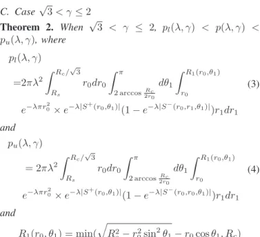
C. Case√3 < γ≤ 2 Theorem 2. When √3 < γ ≤ 2, pl(λ, γ) < p(λ, γ) < pu(λ, γ), where pl(λ, γ) =2πλ2 Z Rc/ √ 3 Rs r0dr0 Z π 2 arccosRc 2r0 dθ1 Z R1(r0,θ1) r0 e−λπr20× e−λ|S + (r0,θ1)|(1 − e−λ|S−(r 0,r1,θ1)|)r 1dr1 (3) and pu(λ, γ) = 2πλ2 Z Rc/√3 Rs r0dr0 Z π 2 arccos2r0Rc dθ1 Z R1(r0,θ1) r0 e−λπr20× e−λ|S +(r 0,θ1)|(1 − e−λ|S−(r0,r0,θ1)|)r 1dr1 (4) and R1(r0, θ1) = min( q R2 c− r20sin2θ1− r0cos θ1, Rc)
Proof: As we have assumed that the node τ0 must
contribute to the triangle bounding the triangular hole to which the origin belongs, the other two nodes must lie in the different half spaces: one in H+ = R+
× (0, π) and the other in H− = R+
× (−π, 0). Since the distance to τ0 is within
Rc, they must also lie in the ball B(τ0, Rc). Furthermore,
they both lie in the area B(0, Rc)\B(0, d0). Therefore, one
node must lie in H+T B(τ
0, Rc)T B(0, Rc)\B(0, d0) and
the other node lie inH−T B(τ0, Rc)T B(0, Rc)\B(0, d0).
Ordering the nodes inH+T B(τ
0, Rc)T B(0, Rc)\B(0, d0)
by increasing polar angle so thatτ1= (d1, θ1) has the smallest
angle θ1. Other nodes such as τ1′, τ1′′ in the same region
have polar angle larger than θ1, as illustrated in Figure 4.
Assume the node τ1 contributes to the triangle bounding the
triangular hole to which the origin belongs, then the third node τ2 ∈ H−T B(τ0, Rc)T B(0, Rc)\B(0, d0) must lie to
the right of the line passing through τ1 and O, denoted by
H+(θ
1). In addition, the distance to τ1 is less than Rc. So
the nodeτ2 must lie in the region
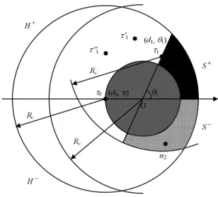
Fig. 4: illustration of case√3 < γ ≤ 2
S−(τ0, τ1) = S−(d0, d1, θ1) = H− \ B(τ0, Rc) \ B(0, Rc)\B(0, d0) \ H+(θ1) \ B(τ1, Rc)
Here we need to obtain the density of nodeτ1. Considering
the wayτ1was defined, there should be no nodes with a polar
angle less than θ1, that is to say no nodes are in the region
S+(τ0, τ1) = S+(d0, θ1) = H+\B(τ0, Rc) \ B(0, Rc)\B(0, d0) \ H+(θ1)
Since the intensity measure of the Poisson process in polar coordinates isλrdrdθ, the density Fτ1 ofτ1can be expressed as
Fτ1(dr1, dθ1) = λr1e−λ|S +
(d0,θ1)|dr
1dθ1 (5)
The integration domain D(d0) with respect to parameters
(d1, θ1) can be easily obtained. According to Lemma 2,
Rs < d0 ≤ Rc/√3. Thus in this case, Rc = γRs ≤
2Rs < 2d0. It means the ball B(τ0, Rc) must intersect with
the ball B(0, d0), as illustrated in Figure 4. Furthermore,
θ0 = 2 arccos(Rc/(2d0)). So 2 arccos(Rc/(2d0))≤ θ1 ≤ π andd0< d1≤ R1(d0, θ1), where R1(d0, θ1) = min( q R2 c− d20sin2θ1− d0cos θ1, Rc)
Assume onlyτ0, τ1 and nodes inS−(τ0, τ1) can contribute
to the triangle bounding the triangular hole to which the origin belongs, we can get a lower bound of the probability that the origin belongs to a triangular hole. It is a lower bound because it is possible that other nodes such as τ′
1, τ1′′ in
H+T B(τ
0, Rc)T B(0, Rc)\B(0, d0) can also contribute to
the triangle bounding the triangular hole to which the origin belongs. Based on the assumption, we have
P{ [ {n1,n2}⊆Φ′r0 T ((r0, π), n1, n2)} > Z Z D(r0) P{ [ n2⊆Φ′r0 T S−(r0,r1,θ1) T ((r0, π), (r1, θ1), n2)}Fτ1(dr1, dθ1) = Z Z D(r0) P{Φ′r0(S −(r 0, r1, θ1)) > 0}Fτ1(dr1, dθ1) (6) Therefore, from (1), (2), (5) and (6), the lower bound shown in (3) can be derived.
Still consider the nodes in H+T B(τ0, Rc)
T B(0, Rc)\B(0, d0), each node (r, θ) corresponds to
an area |S−(r0, r, θ)|. Maybe the corresponding area of
some nodes is 0. Among all such areas, there must exist one maximum value. From Figure 4 , we can see that the closer tor0 is r and the closer to θ1 is θ, the larger is the area of
S−(r 0, r, θ). So we have (r0, θ1) = arg max r0≤r≤R1 θ1≤θ≤π |S−(r 0, r, θ)|
Then the upper bound shown in (4) can be obtained. Here we need to compute the area of S+(r
0, θ1) and
S−(r
0, r1, θ1). In fact, the area |S+(r0, θ1)| and the area
|S−(r
0, r1, θ1)| have very similar expressions. For example,
the area |S+(r0, θ1)| can be expressed as
|S+(r0, θ1)| = Z θ1 2 arccosRc 2r0 dθ Z R1(r0,θ1) r0 rdr =1 2 Z θ1 2 arccosRc 2r0 R21(r0, θ1)dθ− r2 0 2(θ1− 2 arccos Rc 2r0 ) Whenθ1≤ π − arccos(r0/(2Rc)) 1 2 Z θ1 2 arccosRc 2r0
R21(r0, θ1)dθ = I(θ1)− I(2 arccos Rc
2r0 ) where I(θ) =r 2 0 2 sin θ cos θ + R2 c 2 θ− R2 c 2 arcsin r0sin θ Rc −r20sin θ q R2 c− r02sin2θ
Whenπ− arccos(r0/(2Rc)) < θ1≤ π 1 2 Z θ1 2 arccos(Rc/(2r0)) R21(r0, θ1)dθ
= I(π− arccos(r0/(2Rc)))− I(2 arccos(Rc/(2r0)))
+R
2 c
2 (θ1− π + arccos(r0/(2Rc)))
In this way, |S+(r0, θ1)| can be derived. Similarly,
|S−(r
0, r1, θ1)| can be obtained. The detailed process is
ne-glected due to space limitation.
D. Case γ > 2 Theorem 3. When γ > 2, pl(λ, γ) < p(λ, γ) < pu(λ, γ), where pl(λ, γ) = 2πλ2 nZ Rc/2 Rs r0dr0 Z π 0 dθ1 Z R1(r0,θ1) r0 e−λπr20× e−λ|S+(r0,θ1)|(1− e−λ|S−(r0,r1,θ1)|)r 1dr1 + Z Rc/ √ 3 Rc/2 r0dr0 Z π 2 arccosRc 2r0 dθ1 Z R1(r0,θ1) r0 e−λπr20 × e−λ|S+(r0,θ1)|(1 − e−λ|S−(r0,r1,θ1)|)r 1dr1 o (7) and pu(λ, γ) = 2πλ2 nZ Rc/2 Rs r0dr0 Z π 0 dθ1 Z R1(r0,θ1) r0 e−λπr02× e−λ|S+(r0,θ1)|(1 − e−λ|S−(r0,r0,θ1)|)r 1dr1 + Z Rc/ √ 3 Rc/2 r0dr0 Z π 2 arccosRc 2r0 dθ1 Z R1(r0,θ1) r0 e−λπr02 × e−λ|S+(r0,θ1)|(1 − e−λ|S−(r 0,r0,θ1)|)r 1dr1 o (8)
In this case, we can use the same method as in section III.C to get the upper and lower bounds. But we need to consider two situationsRs< d0≤ Rc/2 and Rc/2 < d0≤ Rc/√3. In
the first situation,d0≤ Rc/2 means that the ball B(0, d0) is
included in the ball B(d0, Rc), see Figure 5. Then the lower
limit of integration forθ1is 0. This is the only difference. The
areas|S+(r0, θ1)| and |S−(r0, r1, θ1)| can be computed in the
same way as presented in Section III.C. The second situation is the same as that in section III.C. So we can directly obtain the lower and upper bounds as shown in (7) and (8) respectively.
IV. SIMULATIONS AND PERFORMANCE EVALUATION
This section first introduces simulation settings. Simulation results are then presented and compared with closed form expressions for upper and lower bounds.
A. Simulation settings
A disk centered at the origin with radius Rc is considered
in the simulations. The probability that the origin belongs to a triangular hole is computed. Sensors are randomly distributed in the disk according to a Poisson process with intensityλ. The sensing radiusRsof each node is set to be 10 meters andγ is
Fig. 5: illustration of caseγ > 2
chosen from 2 to 3 with interval of 0.2. So the communication radius Rc ranges from 20 to 30 meters with interval of 2
meters. λ is selected from 0.001 to 0.020 with interval of 0.001. For each γ, 106 simulations are run under each λ to
check whether the origin belongs to a triangular hole.
B. Performance evaluation
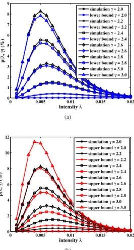
The probabilityp(λ, γ) obtained by simulation is presented with the lower bound and upper bound in Figure 6(a) and 6(b) respectively. It can be seen that for any value ofγ, p(λ, γ) has a maximum at a threshold value λc of the intensity.
As a matter of fact, for λ ≤ λc, the number of nodes is
small. Consequently the probability that the origin belongs to a triangular hole is relatively small too. With the increase ofλ, the connectivity between nodes becomes stronger. As a result, the probability that the origin belongs to a triangular hole increases. However, when the intensity reaches the threshold value, the origin is covered with maximum probability.p(λ, γ) decreases for λ ≥ λc. The simulations also show that λc
decreases with the increase of γ.
On the other hand, it can be seen from Figure 6(a) and 6(b) that for a fixed intensityλ, p(λ, γ) increases with the increases of γ. That is because Rs is fixed. Then the larger Rc is, the
higher is the probability of each triangle containing a coverage hole.
Furthermore, the maximum probability increases quickly with γ ranging from 2.0 to 3.0. It is shown that when Rc = 2Rs, the maximum probability from simulation is about
0.03% and thus it is acceptable to use Rips complex based algorithms to discover coverage holes. While the ratioRc/Rs
is high to a certain extent, it is unacceptable to use connectivity information only to discover coverage holes.
Finally, it can be found in Figure 6(a) that the probability obtained by simulation is very well consistent with the lower bound. The maximum difference between them is about 0.4%. Figure 6(b) shows that probability obtained by simulation is also consistent with the upper bound. The maximum difference between them is about 4%.
0 0.005 0.01 0.015 0.02 0 1 2 3 4 5 6 7 8 9 intensity λ p( λ , γ) (%) simulation γ = 2.0 lower bound γ = 2.0 simulation γ = 2.2 lower bound γ = 2.2 simulation γ = 2.4 lower bound γ = 2.4 simulation γ = 2.6 lower bound γ = 2.6 simulation γ = 2.8 lower bound γ = 2.8 simulation γ = 3.0 lower bound γ = 3.0 (a) 0 0.005 0.01 0.015 0.02 0 2 4 6 8 10 12 intensity λ p( λ , γ) (%) simulation γ = 2.0 upper bound γ = 2.0 simulation γ = 2.2 upper bound γ = 2.2 simulation γ = 2.4 upper bound γ = 2.4 simulation γ = 2.6 upper bound γ = 2.6 simulation γ = 2.8 upper bound γ = 2.8 simulation γ = 3.0 upper bound γ = 3.0 (b)
Fig. 6: proportion of the area of triangular holes (a) simulation results and lower bounds ; (b) simulation results and upper bounds
V. CONCLUSION
In this paper, the proportion of the area of triangular holes in a WSN is analyzed under different ratios between commu-nication radius and sensing radius of each sensor. Both the lower and upper bounds of the proportion are derived. When the ratio is no larger than√3, there is no triangular hole. When the ratio is between √3 and 2, both the theoretical analysis and simulation results show that the proportion is lower than 0.06% under any intensity. It means that the triangular holes
can nearly be neglected and homology based coverage hole detection algorithms can work well if they can discover all non-triangular holes. When the ratio is larger than 2, the proportion of the area of triangular holes increases with γ. It becomes unacceptable forγ larger than a threshold. In that case triangular holes can not be neglected anymore.
REFERENCES
[1] Q. Fang, J. Gao, and L. J. Guibas, “Locating and bypassing routing holes in sensor networks,” in INFOCOM’04, Hong Kong, China, March 2004, pp. 2458–2468.
[2] G. Wang, G. Cao, and T. F. L. Porta, “Movement-assisted sensor deployment,” in INFOCOM’04, Hong Kong, China, March 2004, pp. 2469–2479.
[3] C. Zhang, Y. Zhang, and Y. Fang, “Localized algorithms for coverage boundary detection in wireless sensor networks,” Wireless networks, vol. 15, no. 1, pp. 3–20, 2009.
[4] ——, “Detecting coverage boundary nodes in wireless sensor networks,” in Proceedings of the IEEE International Conference on Networking,
Sensing and Control, ICNSC ’06, Ft. Lauderdale, Florida, USA, April 2006, pp. 868 – 873.
[5] Y. Bejerano, “Simple and efficient k-coverage verification without lo-cation information,” in INFOCOM’08, Phoenix, Arizona, USA, April 2008, pp. 897–905.
[6] V. de Silva, R. Ghrist, and A. Muhammad, “Blind swarms for coverage in 2-d,” in Proceedings of Robotics: Science and Systems, Cambridge, MA, June 2005, pp. 335–342.
[7] V. de Silva and R. Ghrist, “Coverage in sensor networks via persistent homology,” Algebraic & Geometric Topology, vol. 7, pp. 339 – 358, 2007.
[8] R. Ghrist and A. Muhammad, “Coverage and hole-detection in sensor networks via homology,” in Fourth International Conference on
Informa-tion Processing in Sensor Networks (IPSN’05), Los Angeles, California, USA, April 2005, pp. 254–260.
[9] A. Muhammad and M. Egerstedt, “Control using higher order laplacians in network topologies,” in Proc. of 17th International Symposium on
Mathematical Theory of Networks and Systems, Kyoto, Japan, July 2006, pp. 1024–1038.
[10] A. Tahbaz-Salehi and A. Jadbabaie, “Distributed coverage verification in sensor networks without location information,” IEEE Transactions on
Automatic Control, vol. 55, no. 8, pp. 1837 – 1849, 2010.
[11] P. Dlotko, R. Ghrist, M. Juda, and M. Mrozek, “Distributed computation of coverage in sensor networks by homological methods,” 2011. [Online]. Available: http://www.math.upenn.edu/∼ghrist/preprints/
distributedhomology.pdf
[12] B. Liu and D. Towsley, “A study of the coverage of large-scale sensor networks,” in Proceedings of the IEEE International Conference on
Mobile Ad-hoc and Sensor Systems (MASS’04), Fort Lauderdale, Florida, USA, October 2004, pp. 475–483.
[13] P.-J. Wan and C.-W. Yi, “Coverage by randomly deployed wireless sensor networks,” IEEE Transactions on Information Theory, vol. 52, no. 6, pp. 2658 – 2669, 2006.
[14] X. Li, D. K. Hunter, and S. Zuyev, “Coverage properties of the target area in wireless sensor networks,” IEEE Transactions on Information