To cite this document:
Jacob, Christelle and Dubois, Didier and Cardoso, Janette
Uncertainty handling in quantitative BDD-based fault-tree analysis by interval
computation. (2011) In: SUM 2011 - 5th International Conference Scalable Uncertainty
Management, 10 October 2011 - 12 October 2011 (Dayton, OH, United States).
Open Archive Toulouse Archive Ouverte (OATAO)
OATAO is an open access repository that collects the work of Toulouse researchers and
makes it freely available over the web where possible.
This is an author-deposited version published in:
http://oatao.univ-toulouse.fr/
Eprints ID: 10963
Any correspondence concerning this service should be sent to the repository
administrator:
[email protected]
Uncertainty handling in quantitative BDD-based
fault-tree analysis by interval computation
Christelle Jacob1, Didier Dubois2, and Janette Cardoso1
1 Institut Sup´erieur de l’A´eronautique et de l’Espace (ISAE), DMIA department, Campus Supa´ero, 10 avenue ´Edouard Belin - Toulouse
2 Institut de Recherche en Informatique de Toulouse (IRIT), ADRIA department, 118 Route de Narbonne 31062 Toulouse Cedex 9, France.
{[email protected],[email protected],[email protected]}
Abstract. In fault-tree analysis probabilities of failure of components are often assumed to be precise. However this assumption is seldom verified in practice. There is a large literature on the computation of the probability of the top (dreadful) event of the fault-tree, based on the representation of logical formulas in the form of a binary decision diagram (BDD). When probabilities of atomic propositions are ill-known and modelled by intervals, BDD-based algorithms no longer apply to the computation of the top probability interval. This paper investigates this question for general Boolean expressions, and proposes an approach based on interval methods, relying on the analysis of the structure of the Boolean formula. The considered application deals with the fault-tree-based analysis of the reliability of aircraft operations.
Key words: Binary Decision Diagrams, interval analysis, fault-tree
1
Introduction
In aviation business, maintenance costs play an important role because these costs are comparable to the cost of the plane itself. Another important parameter is reliability. A reliable aircraft will have less down-time for maintenance and this can save a lot of money for a company. No company can afford neglecting the reliability and safety of the aircraft, which necessitates a good risk management. Airbus has started a project called @MOST to cater for above mentioned issues. It is focused on the reduction of maintenance costs and hence improving the quality of its products.
This paper deals the probability evaluation of fault-trees through Binary Decision Diagrams (BDDs). This is the most usual approach to risk management in large-scale systems, for which operational software is available. At present, dependability studies are carried out by means of fault-tree analysis from the models of the system under study. This method requires that all probabilities of elementary component failures be known in order to compute the probability of some dreadful events. But in real life scenarios, these probabilities are never known with infinite precision. Therefore in this paper we investigate an approach
to solve cases where such probabilities are imprecise. More specifically, we are concerned with the more general problem of evaluating the probability of a Boolean expression in terms of the probabilities of its literals, imprecisely known via intervals.
2
Dependability studies and fault-tree analysis
One of the objectives of safety analysis is to evaluate the probabilities of dreadful events [?]. There are two ways to find the probability of an event: by an experimental approach or by an analytical approach.
The experimental approach consists in approximating the probability by com-puting a relative frequency from tests: if we realize N experiments (where N is a very large number) in the same conditions, and we observe n times the event e, the quotient n/N provides an approximation of the probability P(e). Indeed, this probability can be defined by: P (e) = lim
N→+∞(n/N ). In practice, it is very
difficult to observe events such as complex scenarios involving multiple, more elementary, events several times.
The analytical approach can be used when the dreadful event is described as a Boolean function F of atomic events. Such dreadful event probability is thus computed from the knowledge of probabilities of atomic events, that are often given by some experts. In a Boolean model of a system, a variable represents the state of an elementary component, and formulas describe the failures of the system as function of those variables. It is interesting to know the minimal sets of failures of elementary components that imply a failure of the studied system, in order to determine if this system is safe enough or not.
If only probability of these minimal sets are of interest, the corresponding Boolean formulas are monotonic and only involve positive literals representing the failures. However, in this paper we consider more general Boolean formulas where both positive and negative literals appear. In fact such kind of non-monotobic formulas may actually appear in practical reliability analysis as shown later.
2.1 The Probability of a Boolean formula
There are two known methods to calculate the probability of a Boolean formula, according to the way the formula is written.
Boolean formula as a sum of minterms A Boolean formula can be written as a disjunction of minterms. By definition, minterms are mutually exclusive, so the probability of a dreadful event is equivalent to:
P (F ) = X
π∈M interms(F )
Boolean methods of risk analysis make the hypothesis that all atomic events are
stochastically independent. So, the previous equation becomes:
P (F ) = X
π∈M interms(F )
Y
Ai∈π
P (Ai) (2)
But this method requires that all minterms of F be enumerated, which is very costly in computation time. In practice, an approximation of this probability is obtained by making some simplifications, namely:
− using the monotonic envelope of the formula instead of using the formula itself [?].
− using minimal cut sets (definition ??) of higher probabilities only.
− using the k first terms of the Sylvester-Poincar´e development, also known as inclusion-exclusion principle (letting each Xi stand for product of literals):
P (X1∨ ... ∨ Xn) = n X i=1 P (Xi) − n−1 X i=1 n X j=i+1 P (Xi∧ Xj) + n−2 X i=1 n−1 X j=i+1 n X k=j+1 P (Xi∧ Xj∧ Xk) − ... + (−1)n+1P (X1∧ ... ∧ Xn) (3)
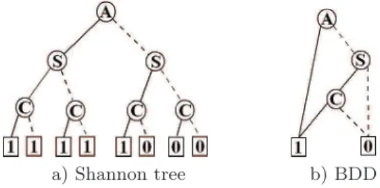
Boolean formula using Shannon decomposition Shannon decomposition consists of building a tree whose leaves correspond to mutually disjoint conjunc-tions of literals.
Definition 1 (Shannon decomposition). Let us consider a Boolean function F on a set of variables X, and A a variable of X. The Shannon decomposition
of F related to A is obtained by iterating the following pattern:
F = (A ∧ FA=1) ∨ (¬A ∧ FA=0) (4)
FA=0and FA=1 are mutually exclusive, so the probability of the formula F is:
P (F ) = (1 − P (A)) · P (FA=0) + P (A) · P (FA=1) (5)
For a chosen ordering of variables of a set X, the recursive application of the Shannon decomposition for each variable of a function F built on X gives a binary tree, called Shannon tree. Each internal node of this tree can be read as an if-then-else (ite) operator : it contains a variable A and has two edges. One edge points towards the node encoded by the positive cofactor FA=1 and the
other one towards the negative cofactor FA=0. The leaves of the tree are the
truth values 0 or 1 of the formula. The expression obtained by the product of variables going down from the root to a leaf 1 is a minterm, and the sum of all those products gives the expression of the formula.
Example 1. The Shannon tree for the formula F = A ∨ (S ∧ C) with order
A > S > C is represented on Fig. 1.a (the dotted edges represent the else). Notice that by convention, edges in Shannon trees are not arrows, but these graphs are directed and acyclic from the top to the bottom.
a) Shannon tree b) BDD
Fig. 1. Formula A ∨ (S ∧ C) with order A > S > C
But such a representation of the data is exponential in memory space; this is the reason why Binary decision diagrams [2] are introduced: they reduce the size of the tree by means of reduction rules.
Binary Decision Diagrams A Binary Decision Diagram (BDD) is a repre-sentation of a Boolean formula in the form of a directed acyclic graph whose nodes are Boolean variables (see Fig. 1.b). A BDD has a root and two terminal nodes, one labeled by 1 and the other by 0, representing the truth values of the function. Each path from the root to terminal node 1 can be seen as a product of literals, and the disjunction of all those conjunctions of literals gives a repre-sentation of the function. For a given ranking of the variables, it is unique up to an isomorphism. The size of the BDD is directly affected by the ranking of variables, and some heuristics can be used to optimize its size.
A variable can be either present (in a positive or negative polarity) in a path, or absent:
− a variable is present in a positive polarity in the corresponding product if the path contains the then-edge of a node labeled by this variable;
− a variable is present in the negative polarity in the corresponding product if the path contains the else-edge of a node labeled by this variable;
− a variable is absent if the path does not contain a node labeled by this variable. Let P be the set of paths in the BDD that reach terminal leaf 1, and Ap the
set of literals contained in a path p of P. If a literal A is present positively (resp. negatively ¬A) in the path p ∈ P, we will say that A ∈ A+
p (resp. A ∈ Ap−).
According to those notations, the probability of the formula F described by a BDD is given by the equation:
P (F ) = X p∈P Y Ai∈Ap+ P (Ai) Y Aj∈Ap− (1 − P (Aj)) (6)
Now assume probabilities are partially known. The most elementary approach for dealing with imprecise BDDs is to apply interval analysis. It would enable robust conclusions to be reached, even if precise values of the input probabilities are not known, but their ranges are known.
3
Interval Arithmetic and Interval Analysis
Interval analysis is a method developed by mathematicians since the 1950s
and 1960s [4] as an approach to computing bounds on rounding or measurement errors in mathematical computation. It can also be used to represent some lack of information. The main objective of interval analysis is to find the upper and lower bounds, f and f , of a function f of n variables {x1, ..., xn}, knowing the
in-tervals containing the variables: x1∈ [x1, x1], ...,xn∈ [xn, xn]. For a continuous
function f , with xi∈ [xi, xi], the image of a set of intervals f ([x1, x1], ..., [xn, xn])
is an interval.
The basic operations of interval arithmetic that are generally used for interval analysis are, for two intervals [a, b] and [c, d] with a, b, c, d ∈ R and b ≥ a, d ≥ c:
Addition : [a, b] + [c, d] = [a + c, b + d] (7) Subtraction : [a, b] − [c, d] = [a − d, b − c] (8) M ultiplication : [a, b] · [c, d] = [min(ac, ad, bc, bd), max(ac, ad, bc, bd)] (9)
Division : [a, b] [c, d] = [min( a c, a d, b c, b d), max( a c, a d, b c, b d)] (10) The equation of multiplication can be simplified for the intervals included in the positive reals: M ultiplication : [a, b] · [c, d] = [ac, bd].
3.1 Naive Interval Computations and Logical Dependency
The major limitation in the application of naive computation using interval arith-metics to more complex functions is the dependency problem. The dependency problem comes from the repetition of the same variable in the expression of a function. It causes some difficulties to compute the exact range of the function. It must be pointed out that the dependency here is a functional dependency no-tion, contrary to emphstochastic dependence assumed in section 2.1 and leading to formula 2.
Let us take a simple example in order to illustrate the dependency problem: we consider the function f (x) = x + (1 − x), with x ∈ [0, 1]. Applying addition (7) and subtraction (8) rules of interval arithmetic gives that f (x) ∈ [0, 2], while this function is always equals to 1. Some artificial uncertainty is created by considering x and (1 − x) as two different, functionally independent, variables.
Consider another example to illustrate the dependency problem on a BDD. We consider the formula of the equivalence F = A ⇔ B = (¬A ∨ B) ∧ (¬B ∨ A) whose BDD is represented by (A ∧ B) ∨ (¬A ∧ ¬B) and pictured on Fig. 2.a.
a) F = A ⇔ B b) G = A ∨ B
Fig. 2. BDD representation
The probability of F knowing that P (A) = a, P (B) = b applying eq. 3 is: P (F ) = a · b + (1 − a)(1 − b) (11) The values of a and b are not known, the only information available is that a ∈ [a, a] and b ∈ [b, b], with [a, a] and [b, b] included in [0, 1].
The goal is to compute the interval associated to P (F ) ∈ [P (F ), P (F )]. If we directly apply the equation of addition(7) and multiplication(9) of two intervals to the expression of P (F ), we obtain that:
[P (F ), P (F )] = [ab, ab]+(1−[a, a])(1−[b, b]) = [ab, ab]+[1−a, 1−a]·[1−b, 1−b])
[P (F ), P (F )] = [ab + (1 − a)(1 − b), ab + (1 − a)(1 − b)] (12) This result is obviously wrong because we use two different values of the same variable (a and a for a, b and b for b) when calculating P (F ) = ab + (1 − a)(1 − b) as well P (F ) = ab + (1 − a)(1 − b).
Now consider G = A ∨ B, with a = P (A) and b = P (B); its BDD represen-tation (Fig. 2.b) is GBDD = A ∨ (¬A ∧ B) with P (GBDD) = a + (1 − a)b, while
the Sylvester-Poincar´e decomposition gives P (G) = a + b − ab. Both P (G) and P (GBDD) display a dependency problem because variable a appears twice with
different signs in these expressions (in P (G) it happens also with b).
3.2 Interval Analysis applied to BDDs
One way to solve the logical dependency problem is to factorize f (x1, ..., xn) in
such a way that variables appear only once in the factorized equation and guess the monotonicity of the resulting function. For the previous example P (G) can be factorized as 1 − (1 − a)(1 − b) where both a and b appear only once. The function is clearly increasing with a and b, hence P (G) ∈ [a + b − ab, a + b − ab], substituting the same value in each place. Unfortunately, it is not always pos-sible to do so, hence we must resort to some alternative ways, by analyzing the function.
Configurations
Given n intervals [xi, xi], i = 1, . . . , n, a n-tuple of values z in the set X =
×i{xi, xi} is called a configuration [11], [7]. An extremal configuration zj, is
the form (xc1
1 , ..xcnn), cn ∈ {0, 1} with xi0= xi and x1i = xi. The set of extremal
configurations is denoted by H = ×i{xi, xi}, and | H |= 2n.
A locally monotonic function f [7] is such that the function, obtained by fix-ing all variables xi but one, is monotonic with respect to the remaining variable
xj, j 6= i. Extrema of such f are attained for extremal configurations. Then
the range f ([x1, x1], ..., [xn, xn]) can be obtained by testing the 2n extremal
con-figurations. If the function is monotonically increasing (resp. decreasing) with respect to xj, the lower bound of this range is attained for xj = xj (resp.
xj = xj) and the upper bound is attained for xj = xj (resp. xj = xj). The
monotonicity study of a function is thus instrumental for interval analysis.
The probability of a Boolean formula
As far as Boolean functions are concerned, some results can be useful to high-light. The goal is to compute the smallest interval [P (F ), P (F )] for the proba-bility P (F ) of a formula, knowing the intervals of its variables. First of all, if a variable A appears only once in a Boolean function F , the monotonicity of P (F ) with respect to P (A) is known: it will increase if A appears positively, and decrease if it appears negatively (¬A). More generally, if a variable A ap-pears several times, but only as a positive (resp. negative) literal, then P (F ) is increasing (resp. decreasing) with respect to P (A). The dependency problem is an important issue for the application of interval analysis in probabilistic BDDs, since terms of the form 1−P (A) and P (A) will in general appear in several places.
Monotonicity of the probability of a BDD representation
One important thing to notice about the formula (6) of probability computation from a BDD, is that it is a multilinear polynomial, hence it is locally monotonic. Let us consider the Shannon decomposition of a formula F for a variable Ai,
i ∈ J1, ..., nK. Formula (5) with A = Ai can be written as: P (F ) = (1 − P (Ai)) ·
P (FAi=0) + P (Ai) · P (FAi=1), where P (Ai) appears twice. It can be written as:
P (F ) = P (FAi=0) + P (Ai) · [P (FAi=1) − P (FAi=0)] (13)
In order to study the local variations of the function P (F ) following P (Ai),
we fix all others Aj,j ∈ J1, ..., nK, j 6= i; the partial derivative of equation 13
with respect to P (Ai) is:
∂P (F ) ∂P (Ai)
= P (FAi=1) − P (FAi=0)
[P (FAi=1) − P (FAi=0)] is a function of some P (Aj), j 6= i, so it does not depend
upon P (Ai), for any i ∈ J1, ..., nK. The monotonicity of function P (F ) with
respect to P (Ai) depends on the sign of [P (FAi=1) − P (FAi=0)]; if constant, the
function is monotonic with respect to P (Ai). We can deduce that if P (Ai) ∈
[a, a], the tightest interval for P (F ) is:
– [P (FAi=0)+a·(P (FAi=1)−P (FAi=0)), P (FAi=0)+a·(P (FAi=1)−P (FAi=0))]
– [P (FAi=0)+a·(P (FAi=1)−P (FAi=0)), P (FAi=0)+a·(P (FAi=1)−P (FAi=0))]
if P (FAi=1) ≤ P (FAi=0)
Knowing the monotonicity of a function makes the determination of its range straightforward. For some functions, the monotonicity can be more easily found in other formats than BDD. But finding the sign of P (FAi=1) − P (FAi=0) is not
so simple, as it depends on some other Aj. If we are able to find this sign for
each variable of the function, we can find its exact (tight) range right away.
Consider again the equivalence connective F = A ⇔ B of section 3.1, where events A and B are associated with the following intervals, respectively [a, a] = [0.3, 0.8] and [b, b] = [0.4, 0.6]. We know that the function is locally monotonic, so the range of P (F ) in eq. 11 will be obtained for the boundaries of the domain of the variables a and b. To find the exact bounds of P (F ), since a and b appear both with positive and negative signs in eq. 11, we will have to explore the 22
configurations:
z1= (a, b), Pz1(F ) = a · b + (1 − a)(1 − b) = 0.3 · 0.4 + 0.7 · 0.6 = 0.54
z2= (a, b), Pz2(F ) = a · b + (1 − a)(1 − b) = 0.3 · 0.6 + 0.7 · 0.4 = 0.46
z3= (a, b), Pz3(F ) = a · b + (1 − a)(1 − b) = 0.8 · 0.4 + 0.2 · 0.6 = 0.44
z4= (a, b), Pz4(F ) = a · b + (1 − a)(1 − b) = 0.8 · 0.6 + 0.2 · 0.4 = 0.56
P (F ) = mini=1,...,4Pzi(F ) = 0.44 and P (F ) = maxi=1,...,4Pzi(F ) = 0.56.
The exact result is P (F ) ∈ [0.44, 0.56], while using expression (12), we find [P (F ), P (F )] = [0.2, 0.9]. If we neglect dependencies, we introduce artificial uncertainty in the result. The exact result is much tighter than the one based on naive interval computation. This is why it is so important to find ways to optimize the bounds of the uncertainty range in interval analysis.
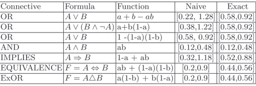
We can compare full-fledged interval analysis applied to all binary Boolean formulas and compare the results with the one obtained by applying naive in-terval computation (Table 1). For those tests, we took the same input proba-bilities as for the example presented in section 3.1, Fig. 2.a: P (A) ∈ [0.3, 0.8], P (B) ∈ [0.4, 0.6]. It is obvious that the two results are the same only when each
Table 1. Comparison between naive interval computation and full-fledged in-terval analysis
Connective Formula Function Naive Exact OR A ∨ B a+ b − ab [0.22, 1.28] [0.58,0.92] OR A ∨(B ∧ ¬A) a+b(1-a) [0.38,1.22] [0.58,0.92] OR A ∨ B 1 -(1-a)(1-b) [0.58, 0.92] [0.58,0.92] AND A ∧ B ab [0.12,0.48] [0.12,0.48] IMPLIES A ⇒ B 1-a + ab [0.32,1.18] [0.52,0.88] EQUIVALENCE F = A ⇔ B ab + (1-a)(1-b) [0.2,0.9] [0.44,0.56] ExOR F = A△B a(1-b) + b(1-a) [0.2,0.9] [0.44,0.56]
variable appears once in the probability P (F ), e.g for F = A ∧ B, P (F ) = ab. For all other cases, we get a tighter interval by testing all extreme bounds of the input intervals. The more redundancy of variables there will be in a formula, the more naive interval computation will give ineffective results, moreover irrelevant in some cases; e.g F = A ∨ B or F = A ⇒ B where we get intervals with values higher than 1. On the contrary, the approach based on local monotony gives the exact range of the Boolean function F .
3.3 Beyond two variables
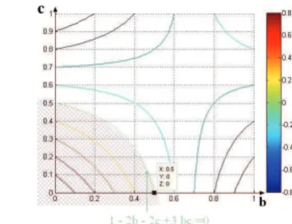
However, the study of monotonicity can be also very complicated. For instance, the function 2 out of 3 is given by the formula:
F = (A ∧ ¬B ∧ ¬C) ∨ (¬A ∧ B ∧ ¬C) ∨ (¬A ∧ ¬B ∧ C)
The partial derivative with respect to a of the probability of this formula is : ∂
∂aP (F ) = (1 − b)(1 − c) − b(1 − c) − c(1 − b) = 1 − 2b − 2c + 3bc Partial derivatives with respect to b and c are similar. It is more difficult to find the sign of such a derivative, because we have a 2-place function that is not monotonic and has a saddle point (see Fig. 3.a). On fig. 3.b we can see the level cuts of the curve, ∂
∂aP (F ) = α.
Fig. 3. a) Partial derivative 1−2b−2c+3bc b) Level cuts of 1−2b−2c+3bc
The derivative is null for 1 − 2b − 2c + 3bc = 0 ⇔ b = 1−2c
1−3c, that is the
equation of an hyperbola. The positive region of ∂
∂aP (F ) is delimited by this
hyperbola, starting from the (0, 0, 1) point.
The study of specific Boolean expressions like the 2 out of 3 can be used as heuristic for computations of more complex formulas.
4
Algorithm for Interval Analysis applied to BDDs
In this section, we will present an algorithm corresponding to the method of imprecise probability computations for BDDs described in the section 3.2. This algorithm is able to compute the exact bounds of the probability of a Boolean function, given the interval ranges of its atomic probabilities.
The input of the algorithm is a Boolean function F where a probability in-terval [v.lb, v.up] is associated to each variable v of F (the lower/upper bound of its probability interval). The variable v of the BDD representation of F is characterized by the following additional attributes: path.value (=0 if the vari-able appears as a positive literal in this path, =1 otherwise) and type ∈ {0,1,2}. The output is a text file with the probability interval of F , [PF.lb, PF.up].
The BDD is represented by a set P a of paths with the following format:
< v1path1: value, . . . , vpath1n1 : value > · · · < vpathm1 : value, . . . , vpathmnm : value > (14)
where m is the number of paths and ni, i = 1, . . . , m is the number of literals
(positive or negative) in a path i. For example, P a = < A: 1 >< S : 0, C : 1 >for
the BDD represented in fig. 1.b.
The algorithm consists of three main steps: in the first step, an Aralia file is parsed for the variables and Boolean formula F of the dreadful event, and a corresponding BDD is generated. In next step, the parsed variables are split into three categories:
− Type 0: Variables that only appear negatively in the Boolean formula − Type 1: Variables that only appear positively in the Boolean formula − Type 2: Variables present in the Boolean formula along with their negation.
We need to find the configuration that represents the minima and maxima for the probability of F. We know the exact values of the bounds of the variables for the 2 first categories from section 3.2, so the configuration is known for these variables:
− if v.type = 0, v.ub is used for calculating PF.lb and v.lb is used for PF.ub,
− if v.type = 1, v.lb is used for calculating PF.lb and v.ub is used for PF.ub,
− if v.type = 2, PF.lb (as well as PF.ub) can be reached for v.lb or v.up, and all
possible extreme values for v must be explored. The total number of these tuples of bounds (configurations) is 2k, where k is the number of variables classified as
Type 2; hence the problem is at most NP-hard.
The last step consists of BDD-based calculations. These calculations are carried out by considering all m paths leading to leaf 1 from the top of the BDD.
Let be zj = (vc1j1, . . . , vcnjn), j ∈ 1, . . . , 2n, ci ∈ {0, 1} a configuration
(sec-tion 3.2). For each configura(sec-tion zj we calculate Pzj(F ) =P (F [v
c1
1j, . . . , vnjcn]).
The extrema are given by P (F ) = mini=1,...,2nPzi(F ) and P (F ) = maxi=1,...,2nPzi(F ).
The notation introduced in eq. 6 is extended to take the category of a variable into account. Let Vl be the set of variables belonging to the path l; Vl2+ (resp.
Vl2−) the set of positive (resp. negative) literals of Type 2 in path l; Vl+ (resp. Vl−) the set of variables of Type 1 (resp. Type 0) in path l.
Let us consider now a configuration (vc1
1 , . . . , v ck
k ) for variables of Type 2,
with v.c = v.lb if vc= 0 and v.c = v.ub if vc= 1:
Cl(v1c1, . . . , v ck k ) = Y v∈V2+ l v.c ∗ Y v∈V2− l (1 − v.c). We have then: P (F ) = X l=1,...,m ( Y v∈V+ l v.lb ∗ Y v∈V− l (1 − v.ub) ∗ min i=1,...,2kCl(v c1 1 , . . . , v ck k )) and P (F ) = X l=1,...,m ( Y v∈V+ l v.ub ∗ Y v∈V− l (1 − v.lb) ∗ max i=1,...,2kCl(v c1 1 , . . . , vkck))
that extends eq. 6 when the probability of the atomic events is given by an interval.
An algorithm that performs the sorting of the variables and computes optimal intervals has been encoded in C++ language, and based on BDD packages named CUDD [3] and BuDDy [8]. BuDDy explores the order of variables in order to optimize the size of the BDD.
5
Application to Fault-Tree Analysis
In Fault-Tree Analysis theory, modelling conventions are generally such that all variables appear only positively in the Boolean formula of the top event: no variable appears with a negation, so the probabilistic formula is monotonic and increasing. But in practice, there are several cases where some variables can appear negatively, and sometimes even both negatively and positively, so that the top formula can be non-monotonic:
– Some negations must be introduced due to compilation: this is clear in BDDs and also in fault-trees obtained from so-called Mode Automata [12]. In this case, the expression is still monotonic as long as the Boolean formula can also be expressed without negative literals (e.g. the connective OR). – State modeling: in some systems, it is necessary to use variables that model
some special states, or modes, which no longer represent a failure, and the global formula may depend on such variables and their negation. It is not necessary increasing with respect to these variables.
– Exclusive Failures: sometimes, failures cannot physically happen simulta-neously, they are then represented by mutually exclusive events or failure modes. Mutual exclusion implies non-monotonicity.
In practice, those kind of variables are very few compared to ”usual” failures; hence, the algorithm will only have NP-hard complexity for them, and be linear for all other variables.
5.1 Case study
The A320 electrical and hydraulic generation systems were the first experiments in model based safety analysis using Altarica language [10], that allows for the
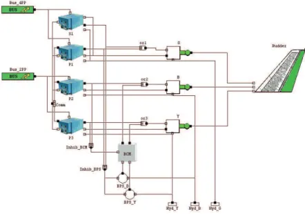
automatic generation of fault trees. The Rudder Control System commands the rudder in order to rotate the aircraft around the yaw axe and is composed of:
– three primary calculators (P1, P2, P3), a secondary calculator (S1) and a emergency autonomous equipment, constituted by a Back-up Control Mod-ule (BCM) and 2 Back-up Power Supply (BPS B, BPS Y),
– three servo-commands: Green (G), Blue (B), Yellow (Y),
– two electric sources (Bus 2PP, Bus 4PP) and three hydraulic sources (Hyd Green, Hyd Blue, Hyd Yellow).
The AltaRica model of the Rudder Control System [6] using the workshop C´ecilia
OCAS from Dassault is presented in fig. 4.
Fig. 4. Rudder’s OCAS model
This model is used for safety analysis and it is has also been used as part of the operational reliability analysis [9]. It is genuinely non-monotonic because of the explicit use of states that doesn’t refer to failures. The failures (elementary events) taken into account are: loss of a component (e.g. B.loss means loss of the Y servo-command), a hidden failure and an active failure (that can occur in S1 and BCM). An excerpt from the generated fault tree in the Aralia format, for the loss of the first primary calculator P1 is given by Fig. 5). Sub-trees are automatically generated and given names (DTN3578, etc.), one per line in the figure.
The probabilities of some variables are known: P(Hyd i.loss)= e−4, P(Bus iPP)=
P1.Status.hs := ((-B.loss & DTN3578) | (B.loss & DTN3617));
DTN3578 := ((-BCM.active failure & DTN3503) | (BCM.active failure & DTN3577)); DTN3503 := ((-BPS B.active failure & DTN3500) | (BPS B.active failure & DTN3502)); DTN3500 := ((-BPS Y.active failure & DTN3483)| (BPS Y.active failure & DTN3499)); DTN3483 := ((-Bus 2PP.loss & DTN3482) | (Bus 2PP.loss & DTN3480));
DTN3482 := ((-Hyd B.loss & DTN3478)| (Hyd B.loss & DTN3481)); DTN3478 := ((-Hyd Y.loss & DTN3475) | (Hyd Y.loss & DTN3477)); DTN3475 := (P1.loss & DTN3474);
DTN3474 := ((-P2.loss & -S1.active failure) | (P2.loss & DTN3473)); DTN3473 := ((-P3.loss & DTN3471) | (P3.loss & DTN3472));
Fig. 5. Excerpt from the fault tree of failure of P1: & is the conjunction, | the disjunction and − the negation.
known: i.[lb,ub] =[0.15, 0.25], i ∈ {Y, B, G}, Pi[lb,ub]=[0, e−2], i = 1, . . . , 3,
S1.Active failure[lb,ub]=[0.1, 0.4] and BCM.Active failure[lb,up]= [0.15, 0.345].
Using the algorithm described in section 4 we obtain the interval I1 =
[0.00676587, 0.027529] for the event Loss of the Rudder represented by F, whereas a wider interval I2= [0.00527422; 0.0356997] is obtained when logical
dependen-cies are not taken into account (applying directly equations (7) and(9) as in equation 12, section 3.1). It can be noticed that the interval I1 is much tighter
than I2.
6
Conclusion
If naive computations using interval arithmetics are applied directly to the BDD-based expression of the probability of Boolean formula, variables and their negation will often appear, and the resulting interval is too imprecise and some-time totally useless. We presented in this paper an algorithm that allows to calculate the exact range of the probability of any formula. We pointed out that there are two cases when a variable and its negation appear in a Boolean expres-sion: the case when there exists an equivalent expression where each variable appear with the same sign, and its probability is then monotonic in terms of the probability of atomic events; the case where such an equivalent expression does not exist. Then this probability will not be monotonic in terms of some variables, and the interval computation is NP-hard.
Even if in practical fault-trees the latter situation does not prevail, the po-tentially exponential computation time can make it inapplicable to very big systems, so some heuristics are under study in order to tackle this issue, for ex-ample, methods to check monotonicity of the obtained numerical functions prior to running the interval calculation, or devising approximate calculation schemes when probabilities of faults are very small.
In future works, our aim is to generalize the approach to fuzzy intervals, using α-cuts. Besides, we must use of reliability laws with imprecise failure
rates, especially exponential laws, so as to generate imprecise probabilities of atomic events. Later on, we can also extend this work by dropping the indepen-dence assumption between elementary faults. One idea can be to use Frechet
bounds to compute a bracketing of the probability of a Boolean formula when
no dependence assumption can be made.
Acknowledgments. This work is supported by the @MOST Prototype, a joint project of Airbus, LAAS, ONERA and ISAE. The authors would like to thank Christel Seguin, Chris Papadopoulos and Antoine Rauzy for discussions about the application.
References
1. M. Siegle: BDD extensions for stochastic transition systems, Proc. of 13th UK Performance Evaluation Workshop, Ilkley/West Yorkshire, July 1997, pp. 9/1-9/7, D. Kouvatsos ed.
2. R. E. Bryant: Graph-Based Algorithms for Boolean Function Manipulation, IEEE Transactions on Computers, C-35(8): 677-691, 1986.
3. F. Somenzi, University of Colorado, http://vlsi.colorado.edu/ fabio/CUDD/ 4. R. E. Moore, R. B. Kearfott, M. J. Cloud: Introduction to Interval Analysis, Society
for Industrial & Applied Mathematics,U.S. 2009.
5. Y. Dutuit, A. Rauzy: Exact and Truncated Computations of Prime Implicants of Coherent and non-Coherent Fault Trees within Aralia, Reliability Engineering and System Safety, 58:127-144, 1997.
6. R. Bernard, J.-J. Aubert, P. Bieber, C. Merlini, S. Metge: Experiments on model-based safety analysis: flight controls, IFAC workshop on Dependable Control of Discrete Systems, Cachan, France, 2007.
7. J. Fortin D. Dubois H. Fargier: Gradual Numbers and Their Application to Fuzzy Interval Analysis, IEEE trans. Fuzzy Systems, 16, 388-402, 2008.
8. http://drdobbs.com/cpp/184401847
9. Tiaoussou, K., K. Kanoun, M. Kaaniche, C. Seguin, C. Papadopoulos: Operational Reliability of an Aircraft with Adaptive Missions. In 13th European Workshop on Dependable Computing, 2011.
10. A. Arnold, A. Griffault, G. Point and A. Rauzy. The altarica language and its semantics. Fundamenta Informaticae, 34:109-124, 2000.
11. R.Moore. Methods and applications of interval analysis. SIAM Studies in Applied Mathematics, 1979.
12. A. Rauzy. Mode automata and their compilation into into fault trees. Reliability Engineering and System Safety, 78 :1-12, 2002.