The Coxeter transformation on cominuscule posets

THE COXETER TRANSFORMATION ON COMINUSCULE POSETS

THESIS

PRESENTED

AS PARTIAL REQ UIREMENT

TO THE PH.D IN MATHEMATICS

BY

EMINE YILDIRIM

UNIVERSITÉ DU QUÉBEC À MONTRÉAL Service des bibliothèques

Avertissement

La diffusion de cette thèse se fait dans le respect des droits de son auteur, qui a signé le formulaire Autorisation de reproduire et de diffuser un travail de recherche de cycles supérieurs (SDU-522 - Rév.0?-2011 ). Cette autorisation stipule que «conformément à l'article 11 du Règlement no 8 des études de cycles supérieurs, [l'auteur] concède à l'Université du Québec à Montréal une licence non exclusive d'utilisation et de publication de la totalité ou d'une partie importante de [son] travail de recherche pour des fins pédagogiques et non commerciales. Plus précisément, [l'auteur] autorise l'Université du Québec à Montréal à reproduire, diffuser, prêter, distribuer ou vendre des copies de [son] travail de recherche à des fins non commerciales sur quelque support que ce soit, y compris l'Internet. Cette licence et cette autorisation n'entraînent pas une renonciation de [la] part [de l'auteur] à [ses] droits moraux ni à [ses] droits de propriété intellectuelle. Sauf entente contraire, [l'auteur] conserve la liberté de diffuser et de commercialiser ou non ce travail dont [il] possède un exemplaire.»

LA TRANSFORMATION DE COXETER SUR LES

ENSEMBLES

ORDONNÉS COMINUSCULES

THÈSE

PRÉSENTÉE

COMME EXIGENCE PARTIELLE

DU DOCTORAT EN

MATHÉMATIQUES

PAR

EMINE YILDIRIM

I would like to thank my supervisor Hugh Thomas for his generous support and for his careful reading of this thesis. His insight and enthusiasm guide me through whole my program. I always admired his intuition, working with him was a great experience.

I would like to thank Thomas Brüstle, Ralf Schiffier, Franco Saliola for reading the thesis and giving me their valuable suggestions.

I would like to thank Institut des Sciences Mathématiques (ISM) for the schola r-ships I received throughout my program. I am grateful for my friends and me n-tors Véronique Bazier-Matte, Nathan Chapelier, Aram Dermenjian, Guillaume Douville, Alexander Garver, Patrick Labelle, Kaveh Mousavand, Rebecca Patrias whom I worked with in working goups at LaCIM. I learned a lot from you! My office mates Aram Dermenjian and Kaveh Mousavand are awesome friends. I val-ued their unlimited support, they were there everytime I needed them. I would like to thank Aram for frequently leaving me encouraging notes around my desk to cheer me up.

I thank my mom Hatice, my father Mühendis, my siblings Fatma, Zeynep, Elif, Harun, and my nephew Eymen for being an amazing and supportive family. Ev-erything becomes fantastic when I share it with them.

Finally, I would like to thank my precious Atabey for his never-ending kindness, support, and his unconditionallove. He never ceases to amaze me with his unique point of view on life.

LIST OF FIGURES RÉSUMÉ . . ABSTRACT INTRODUCTION CHAPTER I PRELIMIN ARIES

1.1 Posets and order ideals

1.2 A quiver and representations of a quiver 1.3 Path algebras . . . . . . . . . . . 1.4 The indecomposable projective modules 1.5 Nakayama functor . . .

1.6 Coxeter transformation . 1. 7 Incidence algebra of a poset CHAPTER II DERIVED CATEGORIES 2.1 Category of complexes 2.2 Homotopy category . . 2.3 Multiplicative systems 2.4 Derived category . . .

2.5 Exact sequences and exact functors 2.6 Resolutions . . .

2.7 Derived functors CHAPTER III Vll lX x 1 5 5 9 11 14

16

17

19

21 21 23 24 25 25 26 29

GROTHENDIECK GROUP AND THE EULER CHARACTERISTIC 31

3.2 Composition series . . . .. . . . . 3.3 Resolutions and the Euler characteristic 3.4 The Grothendieck group of a derived category CHAPTERIV MAIN RESULT 4.1 Projective resolutions . v 32 33 35

39

40 4.2 Action of the Auslander-Reiten translation on the projective resolutions 44 4.3 Intervals in the poset J(P

m

,

n

)

4.4 Homologies and intervals . . .

4.5 Configurations and enhanced partitions . 4.6 The main resul t .

CHAPTER V

A GENERAL FRAMEWORK: COMINUSCULE POSETS

5.1 Refiection along hyperplanes . 5.2 Coxeter groups . . .

5.3 Cominuscule posets . 5.4 Type A 5.5 Type B 5.6 Type C 5.7 Type D 5.8 Exceptional cases CHAPTER VI

MOVIES AND THE PANYUSHEV MAP 6.1 Configurations of dominos . . . . . . 6.2 The movie for a domino configuration . 6.3 The Panyushev map .. . . .. . .

6.4 The short movie for the orbit of the Panyushev map 6.5 The Coxeter transformation and The Panyushev map

45 47 52 56 61 61 63 65 67 70 70 71 77

79

80

86

90

92

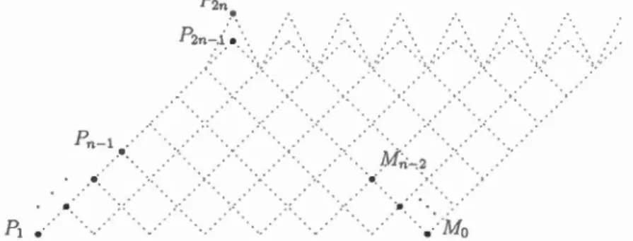
95

6.6 Explicit description of orbits of T and Pan for m

=

2 CONCLUSION . . .. . . .. . . .

96 101 7.1 The second infinite family of cominuscule posets 103 7.2 The Coxeter transformation and the Panyushev map on cominuscule

posets . . . . 107

Figure Page 1.1 The Hasse diagrams of the grid poset P2,3 and the poset of arder

ideals J(P2,_{3 ).} . . . 7 1.2 The Hasse diagram of the poset of arder ideals J(P3,3 ).

4.1 An illustration of the function

f(

a.)

4.2 An illustration of the function

g(a)

5.1 Root poset of A4 . . . • . . . . 5.2 Cominuscule posets of type 1, Il, Ill

5.3 The root poset of An and the cominuscule poset C1 over the simple 8 48 50 63 66 root CJk· . . . 68 5.4 The root poset of Cn and the cominuscule poset C11 over the simple

root (Jn· . . . 71 5.5 The cominuscule poset C111 and the arder ideal poset J(C111) for the

simple root CJ₁ in the root system for Dn. . . . . . . . . . . 72 5.6 An illustration of the module category of D2n and the til ting module

T. .

.

.

. . .

.

. . .

.

. . .

.

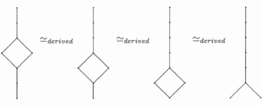
76

5.7 The derived equivalent posets 77

5.8 The cominuscule poset CE₆ and the cominuscule poset CE7 77 6.1 An illustration of a domino configuration.

80

6.2 An illustration of a marked light domino configuration 82 6.3 A domino configuration (I) and the corresponding marked light

domino configuration (II) . . . . . . . . . . . . . 84 6.4 The corresponding movie for a=

(Il

,

1, 2,

3,

31).

89

Vlll

6.5 An orbit of Panyushev map Pan . . . . . . . . . . . . . . . . . . . 91 6.6 The or bit of { -4, -2, 0, 1, 3} under the shift {1} and the

corre-sponding short movie. . . . . . . 94 6.7 Movie and short movie for (0, 1, 1, 3, 3) 96 6.8 An illustration of the order ideal poset J(P(2,n)) 97 6.9 An illustration of sorne orbits of T and Pan in red for J(P(₂,n)) 98 6.10 T-orbit and Pan-orbit in blue for J(P(2,_{9 ))} . . . 99 7.11 An example of a good orbit of T for the poset J(CcJ 104 7.12 An example of a good orbit of T for the poset J(Cc₅) 105 7.13 (1) for J(Cc4 ), (2) for J(Cc5) 106

7.14 (J)for Co4,(JI)for J(CoJ. 107

Soit

J

(C) l'

ensemble ordonné de parties commençantes dans un ensemble ordonné cominuscule C, où C est membre de deux des trois familles infinies d'ensembles o r-donnés cominuscules, ou est un des deux ensembles cominuscules exceptionels. Nous démontrons que la translation de Auslander-Reiten T sur le groupe de Grothendieck de la catégorie dérivée bornée pour l'algèbre d'incidence de l'ensemble ordonné J (

C)

,

qui s'appelle la transformation de Coxeter dans ce cas, a un ordre fini. Spécifiquement, nous démontrons que T(h+l)

=

±id où h est le nombre de Coxeter pour le système de racines pertinent. Écrivant Pan pour l'application de Panyushev, c'est connu que Panh

=

id sur un ensemble ordonné cominus -cule (Rush & Shi, 2013). Nous étudions aussi la relation entre la transformation de Coxeter et l'application de Panyushev.

Mots clés: Théorie des représentations, algèbre d'incidence, la transformation de Coxeter, la translation de Auslander-Reiten, ensemble ordonné cominuscule.

~ - ---- --- --

-Let

J

(C)

be the poset of order ideals of a cominuscule poset

C

where

C

cornes from two of the three infinite families of cominuscule posets or the exceptional cases. We show that the Auslander-Reiten translation T on the Grothendieck group of

the bounded derived category for the incidence algebra of the poset

J

(C),

which is called the Coxeter transformation in this context, has finite order. Specifically, we show that T(h.+l)

=

±id where h is the Coxeter number for the relevant root system. Let Pan denote the Panyushev map. It is known that Panh

=

id on cominuscule posets (Rush

&

Shi, 2013). We also investigate the relation between Coxeter transformation and Panyushev map.

Keywords: Representation theory, incidence algebra, Coxeter transformation, Auslander-Reiten translation, cominuscule poset.

Let A be the incidence algebra of a poset P over a base field !k. If the poset P is finite, then A is a finite dimensional algebra with finite global dimension. We are interested in incidence algebras coming from cominuscule posets. A cominuscule poset can be thought of as a parabolic analogue of the poset of positive roots of a finite root system. Cominuscule posets (also called minuscule posets) appear in the study of representation theory and algebraic geometry, especially in Lie theory and Schubert calculus (Billey

&

Lakshmibai, 2000), (Green, 2013).

Let J ( C) be the poset of order ideals of a given co minuscule poset C. The poset J(C) is an interesting abject in its own right. For instance, there is a corr e-spondence between the elements of J(C) and the minimal coset representatives of the corresponding Weyl group (Billey

&

Lakshmibai, 2000), (Rush & Shi, 2013). Many combinatorial properties of order ideals of cominuscule posets are explained in (Thomas & Yong, 2009). However, our main motivation for this thesis cornes from a conjecture by Chapoton which can be stated as follows.

Let J(ët>+) be the poset of order ideals of ët>+ where ët>+ is the poset of positive roots of a fini te root system éP. Let H be a hereditary algebra of type éP and let TH be the poset of torsion classes. Consider the incidence algebras of J ( ët>+) and TH. Cha po-ton conjectures that there is a triangulated equivalence between the bounded de -rived categories 'Db(modJ(ët>+)) and Vb(modTH) and that 'Db(modJ(ët>+)) is frac -tionally Calabi-Y au, i.e. sorne non-zero power of the Auslander-Reiten translation T equals sorne power of the shift functor.

2

T on the Grothendieck group of the bounded derived category (which is called Coxeter transformation in this context) for Tamari posets is periodic. There is an abundance of studies on Coxeter transformation in the literature. We refer to Ladkani (Ladkani, 2008) for references on the topic and recent results on the periodicity of Coxeter transformation. Kussin, Lenzing, Meltzer (Kussin et al., 2013) showed that the bounded derived category is fractionally Calabi-Y au for certain posets by using singularity theory. Recently, Diveris, Purin, Webb (Diveris et al., 2017) introduced a new method to determine whether the bounded derived category of a poset is fractionally Calabi-Y au.

In this thesis, we consider Chapoton's Conjecture on the level of Grothendieck groups for cominuscule posets instead of root posets. We calculate the action of Auslander-Reiten translation Ton the bounded derived category Db(modJ(C)) of the incidence algebra of the poset J(C) of order ideals of a cominuscule poset C, and then we write the action on the Grothendieck group. We show that the Auslander-Reiten translation T acting on the corresponding Grothendieck group has finite order for two of the three infinite families of cominuscule posets, and for the exceptional cases. One can do this by considering the action of T on any convenient set of generators. The obvious choices are the set of the isomorphism classes of simple modules, and the set of the isomorphism classes of projective modules. However, the periodicity of T is not evident on these sets of generators. Instead, we consider a special spanning set of the Grothendieck group on which we see the periodicity combinatorially.

The plan of the thesis is as follows. In the first chapter, we give necessary back-ground material we use throughout the thesis. In the second chapter, we give a short survey on derived categories, and we prove certain results which are impor-tant in our study. In the third chapter, we give the definition of the Grothendieck group in our setting. We explain the machinery of the Grothendieck group which

we will apply in our study. In the fourth chapter, we introduce a special collection of projective resolutions for grid posets which are the first infinite family of co mi-nuscule posets coming from the type A. Then, we also show the corresponding combinatorics for the homology of these projective resolutions. These projective resolutions provide a spanning set for the Grothendieck group, and in the same section we show that the Coxeter transformation T permutes this collection. In

the fifth section, we study the generalization of our main results for cominuscule posets. The sixth chapter is devoted to developing certain combinatorial tools and using them to show a connection between Coxeter transformation and the Panyushev map. Finally, in the conclusion, we further discuss the second infinite family of cominuscule posets with sorne examples. We also give a brief discussion about the Panyushev map in this context.

PRELIMIN ARIES

In this preliminary section, we will recall basic definitions to fix notation in the thesis.

1.1 Posets and order ideals

A partially ordered set P is a set together with a binary relation :::; which is reflexive, antisymmetric, and transitive. Any partially ordered set P is going to be called a poset throughout this thesis. Two elements a, b are comparable in P if a :::; b or b :::; a, otherwise we say they are incomparable. We say b covers a in P if a

<

b and there is no element c such that a

<

c

<

b. An interval [a, b] in P consists of all elements x such that a :::; x :::; b. A poset P is called locally finite when every interval in P is finite. When P is locally finite, we will represent it by its Hasse diagram, i.e. we represent every element in the poset P by a vertex and we put an edge between two vertices if one covers the other one. We use the convention that the arrows in the Hasse diagram go downwards in the poset even though we simply draw edges in the figures.

6

A chain is a subset of Pin which every pair of elements is comparable. An antichain is a subset of P such that every pair of different elements is incomparable.

Definition 1.1.1. A grid poset Pm,n is the product of two chains of length m and of length n. Explicitly, the elements of P m,n are the pairs ( i, _j) with i E {1, · · · , m} and _j E {1, · · · , n}. We compare elements entry-wise in Pm,n, i.e. (a, b) ~ (c, d) when a ~ c and b ~ d.

A lattice L is a poset such that every pair of elements in L has a unique least upper bound, also called the join, and a unique greatest lower bound, also called the meet. A lattice is distributive if the join and meet operations distribute over each other.

Definition 1.1.2. An arder ideal of a poset P is a subset 1 Ç P such that if bE 1 and a ~ b, then a E 1. We write J(P) for the set of all order ideals of P.

Note that J(P) is always a distributive lattice. Recall that the fundamental the -orem for finite distributive lattices states that if L is a finite distributive lattice, then there is a unique finite poset P such that L ~ J(P) (Stanley, 2012).

Definition 1.1.3. A non-decreasing finite sequence of positive integers (a1, . . . ,

am)

is called a partition. We are going to represent su ch sequences by a

=

(>,~1_,

· · · , À~r) where 0 ~ À1

<

· · ·

<

Àr ~ n denote the distinct integers in the partition a while

a/s denote the number of repetitions of each Ài·

For each k E {1, ... , m}, by the k-th row of Pm,n we mean elements of the form

(

k,

b

)

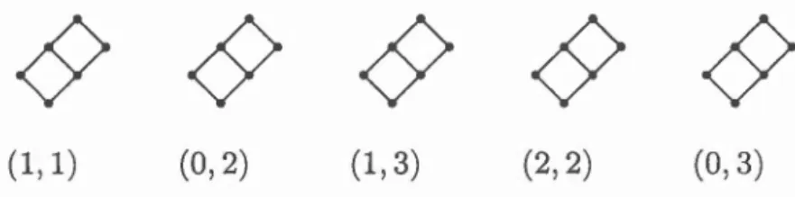
in Pm,n· We represent an order ideal l in J(Pm,n) by its corresponding pa rti-tion, i.e. the list of the number of elements of 1 in each row from top to bottom. Example 1.1.4. Here is an example of a grid poset and its poset of order ideals with the corresponding partitions:

(3,3)<5<

~

(2,3)<):'

/

~

(2,2)<> (1, 3 ) " ' /

~/~

(1, 2)

·

v

(0,

3v

/

~/

(1, 1) ~ (0, 2) /

~/

(0, 1) • (0,0) 0 /

Figure 1.1 The Hasse diagrams of the grid poset P2,3 and the poset of order

ideals

J

(P2

,

3).

For instance, take the order ideal 1 represented by the partition (2, 3) in J(P2 ,3 ). The order ideal 1 consists of two rows: there are two elements in the first row, and

we have three elements in the second row.

Example 1.1.5. This example shows the poset of order ideals in P₃,₃. We draw sorne of the edges with dotted lines for the sake of presentation.

8

<8>(3,3,3)

1.2 A quiver and representations of a quiver

A quwer consists of four p1eces of information ( Q0 , Q1, s,

t)

:

Q

0 is the set of vertices,

Q

1 is the set of arrows between vertices, and s,

t :

Q1

-t

Q

0 are two maps on the arrows where s sencls an arrow to its starting vertex, call it source

and t; sends an arrow to its ending vertex, call it target.

A quiver is said to be finite if

Q

0 and

Q1

are finite sets. Two arrows ex and fJ are

composable if t(cx)

=

s(fJ), and we write the composition as concatenation of ex

and fJ, cxfJ. A pa th in

Q

is a sequence of composable arrows. A pa th of length greater than or equal to one is called a cycle if its source and target coïncide. A cycle of length one is called a loop. A quiver is acyclic if it contains no cycles. For every vertex v in

Q

0, we define the lazy path at v to be the path of length 0 at a vertex v. Let lk be a ground fi ld. A relation in

Q

is a lk-linear combination of path of length at least two, with the same source and the target.

All vector spaces we mention are over !k. A quiver representation M

=

(Vi

,

f

a

) is

a collection of vector spaces

Vi

for each vertex i E

Q

₀

and linear maps

f

a :

Vi

-t Vj for every arrow a : i -t j E

Q

_{1 .} If each vector space

Vi

is finite-dimensional, then

M is called finite-dimensional. In this case, we define the dimension vector of M

as dim(M) = (dim

Vi)

iEQo

where dim

Vi

denotes the dimension of the vector space at vertex i E Qo.

Let lV!

=

(Vi

, f

a)

and N

=

(Wi, g

a

)

be two representations of a quiver Q. We define a morphism of representations

cp

: M

-t N as a collection of linear maps ( c/Ji)iEQo such that for every arrow a E Q1 the following diagram commutes:

10

'\!Ve define Rep(

Q)

to be the category of lk-linear representations of

Q

and their morphisms and rep(

Q)

as the full subcategory of Rep(

Q)

consisting of fini te di-mensional representations. Both Rep(

Q)

and rep(

Q)

are abelian categories. A quiver representation M is said to be indecomposable if J\1! is nonzero and lVI has no direct sum decomposition lVI ~ N EB L, where L and N are nonzero representations of the quiver.

We recall here a fundamental result, the Krull-Schmidt theorem, in representation theory.

Theorem 1.2.1. (Etingof et al., 2011, Theorem 2.19) Any finite dimensional representation can be uniquely decomposed into a direct sum of indecomposable representations up to an isomorphism and arder of summands.

Example 1.2.2. (Etingof et al., 2011) Let us now discuss the indecomposable representations of the A₃ quiver with the following orientation.

A3: • ~ •~•

A representation of this quiver looks like

In total, for A₃ qui ver, we have six indecomposable representations as listed below:

lk~o~o , o~o~lk ,

lk~lk~o , lk~lk~lk ,

Example 1.2.3. Let

Q

be the quiver • ~ • ~ • and X and Y be the repr

e-. 1 1 1 0 ( )

sentatwns; lk ~ lk ~ lk and lk ~ lk ~ 0 . Let us show that Hom X, Y is the one-dimensional and Hom(Y, X) =O.

~ : ~

À À 0

y y y

lk _.,._2_ lk ~ 0

The only morphisms are as shawn. This shows that Hom(X, Y) = lk

À' J-L' 0 ~

y

y

y

lk _.,._2_ lk ~ lk

The only values for À and J.L which make the diagram commute are À

=

J.L

=

O. From this, we can easily see that Hom(Y, X) =O.

1.3 Path algebras

Let

P

(

Q) be the set of all paths over a qui ver Q. We define the path algebra of the quiver Q as A= lkQ := spank(P(Q)) with a lk-linear multiplication J.L: A x A---+ A as follows { pq J.L(p, q) = 0 if s(q) = t(p) otherwise

where p, q E P( Q). This multiplication is unital (unit being the sum of lazy paths) if

Q

₀ is finite, and it is associative.

Lemma 1.3.1. (Assem et al., 2006) The path algebra A

=

lkQ is finite dime

12

Assume that A is a finite dimensional lk-algebra. An element e E A is called an idempotent if e2

₌

_{e. A finite list of idempotents { e}

1, · · · , en} is called a complete set of primitive pairwise orthogonal idempotents if

3. ei cannot be written as a sum of two nontrivial orthogonal idempotents,

The algebra A is called basic if eiA ~ ej A for all i =!= j. For instance, the pa th algebra lkQ satisfies these conditions; ei 's are the vertices, in other words paths of lenght zero.

Let J be the two-sided ideal of the path algebra A

=

lkQ generated by the arrows of Q. A two-sided ideal 1 of A

=

lkQ is called admissible if there exists m

2':

2 such that

J

m

Ç 1 Ç

J2

where

J

i

,

2 :::; i :::; m is the two-sided ideal generated by paths of length greater or equal to i.

Example 1.3.2. Let the quiver

Q b

e defined as

In this case, the set of paths is

P(Q)

=

{e,

f

,

g,

h

,

x, y, z,

t

,

xy, zt}. Sorne examples of admissible ideals are spanr.. { xy}, spanr.. { zt}, spanr.. { xy, zt}, spanr.. {x y- zt}. The vector space spank{x, xy, zt} is an example of a non-admissible ideal.

Proposition 1.3.3. (Assem et al., 2006) Let Q be a finite quiver with admissible

ideal I in

lkQ,

th en lkQ

1

I is finite dimensional.

Let (

Q,

R) be the qui ver with a set of relations R which consists of sorne linear combination of paths of at least length two, with the same source and the target. We call

(Q,

R) a bound quiver. Let rep(Q, R) be the full subcategory of rep(Q)

consisting of the representations of

Q

bound by the relations in R.

Theorem 1.3.4. (Assem et al., 2006) Let Q be a finite connected quiver and

I be an admissible ideal of

lkQ.

There is an equivalence between the category

mod A of right modules over the algebra A

= lkQ

1

I and the category rep( Q,

I)

of

representations of a quiver Q bound by I.

The equivalence of these categories is given by the following functors:

F : mod A -t rep( Q,

I)

and G : rep(

Q

,

I)

-t mod A

For a module M E mod A, F(M)

=

(Vi

,

fa)iEQo,aEQ₁ where

Vi

=

M ei which is the vector space consisting of all vei for all v E M and fa :

Vi

-t

Vj

is defined as

follows: for every arrow a : i -t j

{

va if s(a)

=

i

fa(vei)

=

v(eia)

=

0 otherwise.

For every map <jJ : M -t M' in mod A, F( <jJ) is the morphism defined as </Ji : Mi -t M; for the vertex i which sends vei ~ <j;(v)ei·

For a quiver representation V=

(Vi

,

fa)iEQo,aEQ₁, G(V) = M where M = EBiEQo

Vi

with the action of A is defined as follows: for v

= (

vi)iEQo E M, and s

=

14

L

6cc

+

1

E

A

where

c

runs over all paths in

Q,

vs

=

L

O

c

f

c(v

)

where

f

e( v)

=

(0, · · · , 0,

f

c

(vs(c)), 0,

· · · , 0) with the only nonzero entry in

t(

c).

For every map '1/J

=

('1/Ji)iEQo :

(Vi

,

.fa) --7

(V:'

,

f~), G('l/J) : V --7 V' defined by

G(f)(m)

=

('1/Ji(vi))iEQo·

1.4 The indecomposable projective modules

We first recall the following.

Definition 1.4.1. An A-module X is called decomposable if it can be written as a direct sum of two non-trivial A-modules as X

=

Y EB Z. Otherwise, it is called indecomposable. A module X is called simple if it has no non-trivial submodules.

Note that each simple module is indecomposable, but the converse need not be

true.

Let i be a vertex of the qui ver Q. We define Pi to be the indecomposable projective

module at the vertex i which is spanned by the set of all paths starting at i. Let

us use xi?.j to denote the unique path that starts at vertex i and ends at vertex j. Then, the morphisms between two indecomposable projective modules Pi and Pj are

By definition, Pi is a subspace of lk.Q. But, it is also a submodule, and there -fore, it is a right ideal. We also have a decomposition of lk.Q as a direct sum of

indecomposable modules as

lk.Q =

E9

Pi =

E9

eilk.Q

iEV iEV

Let A

=

lk.Qj I be a quotient of a quiver algebra with lk.Q an admissible ideal!. If the algebra A is finite dimensional, the algebra A viewed as a right module over

itself, then it admits a direct sum decomposition

where Pi

=

eiA are projective indecomposable modules which are also ideals and the ei 's are a set of primitive pairwise orthogonal idempotents of A su ch that

1 = :2:~=

1

ei· This is a decomposition of A as a sum of indecomposable summands. Example 1.4.2. Let

Q b

e the quiver depicted as follows:

. 1 ---i>-• 2 ---i>-• 3

Then the indecomposable projective modules are

p3 :

0 ---i>-0 ---i>-lk

Example 1.4.3. Let

Q b

e the quiver depicted as follows:

16

\Ve define Ji to be the indecomposable injective module at the vertex i which is spanned by the set of all paths ending at i. The simple module Si at vertex i is spanned by the lazy path at i. For a more detailed description of indecomposable projective, injective and simple modules over a quotient of a path algebra, see (As sem et al., 2006), ( Schiffier, 2014).

1.5 Nakayama functor

Let A = kQ/ 1 be a quotient of a quiver algebra kQ with an admissible idealJ.

Definition 1.5.1. The endofunctor v= DHomA(-,A) on modA is called the Nakayama functor where D

=

Homk( -, k) is a duality between left and right A-modules.

Lemma 1.5.2. The Nakayama functor v is right exact and is functorially iso-morphic to - ®A DA.

Proof. The functor D is contravariant exact, and HomA (-,A) is a contrava ri-ant left exact functor. So, their composition v is right exact. The isomorphism between v and - ®A DAis given by the following map.

c/J:

X ®A DA--+ DHomA(X, A)

with x Q9 f f--7 ('lj; f--7 f('lj;(x))) where xE X , fE DA, and 'ljJ E HomA(X, A). 0

Let proj A be the full subcategory of mod A whose abjects are the projective modules and inj A be the full subcategory of mod A whose abjects are the injective modules.

Lemma 1.5.3. The Nakayama functor v induces an equivalence between proj A and inj A. The quasi-inverse of this equivalence is v-1

=

HomA(DA,-) from inj A to proj A.

Proof. Let Px be the indecomposable projective module exA where ex is the idempotent at vertex x. Then, we have vPx

=

DHomA(exA, A) ~ D(Aex)

=

Ix where Ix is the injective module at vertex x. Similarly, we can show that HomA(DA, Ix)= HomA(DA, D(Aex)) ~ HomAo~'(Ae:c, A)~ exA =Px· 0

1.6 Coxeter transformation

Definition 1.6.1. Let A be a basic finite dimensional algebra with a complete set { e1, e2, · · · , en} of primitive orthogonal idempotents. The Cartan matrix CA

of A is the n x n matrix

Cn., 1 Cn.,2 Cn,n where Cji

=

dimlk eiAej, for i, j

=

1, · · · , n.

Example 1.6.2. Let Q be the same quiver as in 1.3.2. We consider the path algebra A

=

lkQ

/

I where I is the ideal generated by the relation

<

xy -

z

t

>.

Then, the Cartan matrix is

1 0 0 0 1 1 0 0

CA=

1 0 1 0 1 1 1 1

The following lemma states that since we have the isomorphisms

eyAex ~ HomA(Px, Py) ~ HomA(Ix, Iy)

the Cartan matrix CA records the number of lin earl y independent homomorphisms between the indecomposable projective modules and the number of linearly in de-pendent homomorphisms between the indecomposable injective modules.

18

Lemma 1.6.3. We have the following properties for the Cartan matrix CA;

1. The i-th column of CA is the dimension vector dim Pi of the indecomposable

projective Pi,

2. The i-th row of CA is the transpose of the dimension vector dim Ii of the indecomposable projective Ii.

Definition 1.6.4. The Coxeter matrix of Ais defined as <I> A

=

-C~ C_41. The c or-responding linear transformation <])A:

zn

--+

zn

defined by matrix multiplication

<])A (x)

=

<]) AX for all x E

zn

is called the Coxeter transformation.

Notice th at sin ce dimension vectors are elements of

zn

,

we can apply the Coxeter transformation on dimension vectors.

Example 1.6.5. We continue with Example 1.6.2. In this case, the Coxeter

matrix is the following

0 0 0 -1 0 0 1 -1 0 1 0 -1

- 1 1 1 - 1

Lemma 1.6.6. <I> A dim Pi=-dim Ii.

Prooj. Let dim Si be the dimension vector of the simple module at vertex i. So,

we have the following by Lemma 1.6.3

<])A dim pi= -C~C_41 dim pi= -C~ dim si=-dim Ii

0

Observe that we have <I> A dim Pi

=

-

dim v Pi for every projective module Pi since vPi =

h

1. 7 Incidence algebra of a poset

For a given locally finite poset P, we define the incidence algebra of P as the path

algebra of the Hasse diagram of P modulo the relation that any two paths are

equal if their starting and ending points are the same. Recall that we draw edges

in the Hasse diagram oriented downwards.

Throughout this thesis, let

A

be the incidence algebra of J(Pm,n)· The algebra

A

has finite global dimension since we do not have any oriented cycles in the quiver

of

J

(

P m,n). Let mod

A

be the category of fini tel y generated right modules over

A

.

Let Po. be an indecomposable projective module over the algebra A for a vertex

a in J ( P m,n) and denote Xo.?J3 the unique pa th th at starts at vertex a and ends at

DERIVED

CATEGOR

I

ES

Our treatment of the subject follows Krause's Chicago Lectures on derived cate

-gories (Krause, 2007). Let lk be a ground field, and let A be a fini te dimensional

unital algebra over !k. We will use mod A to denote the category of fini te dime

n-sional right A-modules.

2.1 Category of complexes

Throughout this thesis, we will use the cohomological convention for complexes: all differentiais increase the degree by one and we use superscripts to denote the

degree at which the module is placed in the complex.

Definition 2.1.1. A chain complex C over an algebra A is defined as a diagram

of A-modules and morphisms of A-modules

Cn-1 dn-1

en

dn cn+l

.

.

.

--+

---+

---'+

--+

...

such that

dn+ldn

=

0 for all n E Z.

Definition 2.1.2. The n-th homology

H

n(C)

of a complex

C

is defined as follows:

22

Definition 2.1.3. A chain map between two complexes e and D is a sequence

of maps f

=

un : en

---+

n n )na su ch that the following diagram commutes:

en-1 dn-1 en dn en+1

· ·· ~ ~ ~ ~···

r

-

1

1

r

l

r+l

l

... ---r n n-1 ---r n n ---r n n+ 1 ---r . . .

dn-1 dn

The lk-vector space of chain maps between two complexes

e

and D is denoted by Hom(e,

D)

, and

the category of chain complexes of A-modules is denoted by e h(A).

Definition 2.1.4. A complex e in Ch(A) is called bounded below if there is an

index N E Z su ch th at Cn

=

0 for every n ~ N. Similarly, e is called bounded above if there is an N E Z su ch that en

=

0 for every n

2':

N. Finally, a complex e is called bounded if it is both bounded below and bounded above. The subcategory of bounded above complexes is denoted by eh_(A), the subcategory of bounded below complexes is denoted by eh+(A), and finally the subcategory of bounded complexes is denoted by e hb(A).

Proposition 2.1.5. The n-th homology is a functor of the form Hn: e h(A)

---+

modA.

Proof. Assume ( e, de) and

(D

,

dD) are complexes in eh( A), and let

f:

e

---+

D

be a map of complexes. By definition,

for every n E Z. Th en there is a well-defined map Hn (.f) : Hn ( e)

---+

Hn (

D)

.

The fact that Hn(idc) is the identity map, and that Hn(gf)

=

Hn(g)Hn(f) for a pair of composable map of complexes,

f

E Hom(e, D) and g E Hom(D, E), and for

every n E Z follows from the definitions. 0

-2.2 Homotopy category

Definition 2.2.1. We say a chain map f : e ---7 D is null-homotopic if there is a sequence of maps h

=

(hn : en ---1 Dn-l) such that for the following diagram

. .. ______,._ en-1 ~ en ~ en+ 1 ______,._ ...

r-1

l

7tn

1

h/

l

r+l

. . . ______,._ Dn - 1 ______,._ Dn ______,._ Dn+ 1 ______,._ . . .

dn-1 dn

we have

.r

= dn_1hn

+ h

n+1dn for all n E Z. If we have two chain maps f, g,

then we say f is homotopie to g if f - g is null-homotopic. The chain map h is

called a homotopy.

Definition 2.2.2. A collection of chain maps I in the category eh(A) is called a right ideal if for every morphism

f

E Hom( e , D) in eh( A) and every morphism g E Hom(D, E)

nI

the composition gf is also in I . Left ideals and two sided ideals are defined similarly.

Lemma 2.2.3. Let I be a two sided ideal of eh(A). The quotient category

eh( A)

j

i

which shares the same set of abjects with morphisms are defined as

quotients

Hom(e, D)/I(e, D)

is a lk-linear category.

Proof. The fact that each Hom object for the quotient is a lk-vector space and

compositions are lk-bilinear is obvious. The fact that the compositions are we

ll-defined follows from the fact that I is a two sided ideal. 0

Proposition 2.2.4. The subcategory Null(A) of null homotopie maps is a two

sided ideal in eh( A). The quotient category eh( A)/ N ull (A) is called the homo-topy category of chain complexes of A-modules, and is denoted by K(A).

24

The corresponding subcategories of bounded above, bounded below and bounded

complexes are denoted by K-(A), K+(A), and Kb(A), respectively.

2.3 Multiplicative systems

Definition 2.3.1. A subcategory S of K(A) is called a a multiplicative system if

(i) For every s E S(C, D) and f E Homi<(A)(C, C'), there are morphisms

s' E S(C', D') and

f'

E HomK(A)(D, D') such that the following diagram

is commutative:

C'~D'

s'

(ii) For every s E S(C, D) and g E Homi<(A)(D', D), there are morphisms

s' E S( C', D') and g' E Homi<(A) ( C', C) such that the following diagram

is commutative:

C'~D'

s'

(iii) For every s, tE S(C, D), there is a f E Homi<(A)(D, D') with fs =ft if and

only if there is agE Homi<(A)(C', C) such that sg =tg.

Theorem 2.3.2. (Gabriel & Zisman, 1967) AssumeS is a multiplicative system in K(A). Then, there is a category

s-

1 _{K(A) in which morphisms of S are all}

2.4 Derived category

Definition 2.4.1. A map of complexes f is a quasi-isomorphism if f induces

isomorphisms in all homology groups, i.e.

Hn(f): H

n(

C) ---7

Hn(D)

is an isomor-phism for every n E Z.

Proposition 2.4.2. (Krause, 2001, Sect. 3.1) The subcategory of quasi-isomorphisms

Q(A) of K(A) forms a multiplicative system. The resulting localization Q(A)-1 K(A)

is called the (unbounded) derived category of A-modules, and is denoted by D(A).

The corresponding derived subcategories of bounded above, bounded below and bounded complexes are denoted by v -(A), v +(A), and Db(A), respectively.

2.5 Exact sequences and exact functors

Definition 2.5.1. A composable pair of morphisms of A-modules X

~

Y .!!....t Z is

called an exact sequence if Ker(g) =lm(!). Note that for such an exact sequence X = 0 if and only if g is injective, and Z = 0 if and only if

f

is surjective. Similarly,

0---+X~Y---+0

is an exact sequence if and only if f is an isomorphism.

A composable pair of morphisms of A-modules of the form 0 ---7 X

~Y

.!!....t Z ---7 0 is called a short exact sequence if it is exact and f is injective, g is surjective. With this definition in hand, we see that a complex C is acyclic when C viewed as a sequence of morphisms

dn-1 C dn C dn+l

· · · ~ n ----'7 n+l ~ · · ·

26

Definition 2.5.2. Assume F: mod A -+ mod B is a functor. Then F is called

right exact if every short exact sequence of A-modules 0 -+ X

-4

Y

!4

Z -+ 0 is

mapped to an exact sequence of the form

F(X) F(J) F(Y) F(g) F(Z) -+ 0,

and similarly, F is called lejt exact if we have an exact sequence

0-+ F(X) F(J) F(Y) F(g) F(Z).

Such a functor is called exact if it is both left and right exact.

Example 2.5.3. Assume M is a left A-module and a right B-module such that

(a· m) · b = a· (m · b)

for every m E M, a E A and b E B. The functor F : mod A -+ mod B from the category of right A-modules to the category of right B-modules defined on the abjects as F(X) = X ®A M is right exact. On the other hand, G(X) =

HomA (X, M) defines a left exact contravariant functor from the category of left

A-modules to the category of right B-modules.

2.6 Resolutions

We start recalling sorne definitions.

Definition 2.6.1. An A-module P is called projective if for every epimorphism

of A-modules h: X -+ Y, every morphism of A-modules f : P -+ Y lifts to a

morphism g: P -+ X such that the following diagram commutes:

9 ;:.··

x

---+

y

---+ 0 h

Similarly, we call an A-module E injective if for every monomorphism of

A-modules h: Y ---+ X , every morphism of A-modules

f

:

Y ---+ E lifts to a morphism g: X ---+ E such that the following diagram commutes:

E J ·· ... g

l

"'

0 - - - ? -

y

- - - ? -

x

h

Definition 2.6.2. For a module M from mod A, by the stalk complex of M we mean the complex which consists of just M at one degree and 0 everywhere else. Definition 2.6.3. For a module M from modA, by a resolution of M we mean a

complex X= (Xi)iEZ where Xi = 0 for all i

>

0 or for all i

<

0 with the property that the homology

H

0

_(X)

_is

_M

_while

_H

_n

_(X)

_{is zero for all n}

_=/=O

_.

If X is bounded from above and each Xi is projective, then X is called a projective

resolution. Similarly, if X is bounded from below and each Xi is injective, then

X is called an injective resolution.

Notice that if X is a projective resolution of a module X, then the natural surjec -tion X ---+ X of complexes is a quasi-isomorphism. Similarly, ifE is an injective

resolution of X , then the natural injection X---+

E

is also a quasi-isomorphism.

Lemma 2.6.4. Assume

f:

X---+ Y is a morphism of A-modules. Assume X is a projective (respectively, injective) resolution of X, and

Y

is a projective

(respec-tively, injective) resolution ofY. Then there is a unique (up to a homotopy) chain

map of complexes of the form

f*:

X---+

Y

such that H0(f*)

=

f .

Proof. We give the proof below for the projective case only. The proof for the

injective case is similar, and we omit it. Since X is a resolution of X and

Y

is a resolution of Y, there are epimorphisms of A-modules Px: X0 ---+ X and

28

py: Y0 _{---7 Y. Then there is a commutative square}

X0 _~X

y

Jo

lJ

yo---+ y

py

Here

J

0 _{lifts the morphism}

_Jo

_{Px· Since the square above is commutative,}

_J

0

restricts to a morphism of the form

J

0

: Ker(p x) ---7 Ker(py). Sin ce both X and

Y

are resolutions, we must have Ker(px) = lm(d_{_1)} and Ker(py) = lm(d_{_1).} So, we now have -1 d-l l (d ) X __,... m -1

•rl

y

1

Jo

y -1 _____,._ lm(d-1) d-1

where this time

J

-

1 lifts the composition

J

0_{d_}

1 . Now, we proceed by induction to

get the chain map f*. As for our second claim, assume we have two lifts f* and

g* for the same morphism of A-modules

J:

X ---7 Y. Then, we geta commutative

diagram of the form

x

-

1

d-1

xo

PX X

rl-g

-

11

... ··

.

'~o

.

/··

lJo-go

la

y-1 ""' " d-1 ./ yo y

~

~/

py lm(d- 1) where

1. the lift X0 _{---7 lm ( d-}1) ex_{ists because lm ( d- 1)}

₌

_{Ker (py) and py o (!}0

- g0)

=

0,

2. the lift h0_{: X}0 _{---7 y-}1 _{exists because X}0 _{is projective and y-}1

---7 lm(d- 1)

Note that we do not necessarily have h0_d-1

₌

_f

_-

1 _{- g-}1

, but we have

Thus, we get a lift of j-1 _{- g-}1 _{- h}0_d-1_:

x-

1

_--t

y

-

1 _{first to}

x-

1

_--t

_Im(d-2₎

then to h-l: x -l

--t

y -2 that satisfies

Proceeding by induction, we get maps hi :

X

i --t

yi-l such that

for every i E N which gives us the desired null homotopy. 0

2.7 Derived functors

Definition 2. 7 .1. Assume F: mod

A

--t

mod

B

is a right exact functor. For every

p E N we define the left derived functor

V

F: mod

A --t

mod

B

as

V F(X)

:=

H

P

(F(X))

where

X

is any projective resolution of

X.

Note that

LP

F

is

well-defined because of Lemma 2.6.4, and that

L° F

=

F

since

F

is right exact. Example 2.7.2. Recall that for a A-B-bimodule M, the functor _ ®AM defines a right exact covariant functor from the category of right A-modules to the

cat-egory of right B-modules. The left derived functors of _ ®A M are denoted by

Tor~(_, M).

Definition 2. 7.3. Assume G: mod

A--t

mod Bis a left exact functor. For every

p E N we define the right derived functor

RPG:

mod

A

--t

mod

B

as

RP

G(X)

:=

HP(G(X))

where

X

is any injective resolution of

X.

Note that, again,

R

P

G

is well-defined because of Lemma 2.6.4, and that R0_G

₌

_{G since Gis left exact.}

30

Example 2.7.4. Recall that for an A-B-bimodule

!VI,

the functor

HomA(_,

M)

defines a left exact contravariant functor from the category of left A-modules to the category of right B-modules. The right derived functors of

HomA (_,Nf)

are denoted by Ext~(_,

M).

GROTHENDIECK GROUP AND THE EULER CHARACTERISTIC

Throughout this chapter, we assume A and B are finite dimensional lk-algebras, and we use mod A and mod B to denote the categories of fini te dimensional right A and B-modules. We also assume C is a subcategory of mod A.

3.1 The definition

Definition 3.1.1. The Grothendieck group K₀(C) of C is defined to be the abelian group generated by isomorphism classes of objects in C divided by the relation

[X] - [Y]

+

[

Z] for every short exact sequence 0 -+ X -+ Y -+ Z -+ 0 in C.

Theorem 3.1.2. Assume F: mod A-+ mod B is an exact functor. Then F

in-duces a map of Grothendieck groups of the form K0(F): K0(mod A) -+ K0(mod B).

Proof. Any functor sends an isomorphism to another isomorphism. Moreover, F

sends short exact sequences to short exact sequences since

F

is also exact. Then K0(F)[X]

=

[F(X)] is well-defined for every A-module X. D

32

3.2 Composition series

Definition 3.2.1. We say that an object X in mod A admits a composition series in C if there is a sequence of submodules

Xo C · · · C Xn =X

such that X0 E C and each Xi+I/Xi E C. We are going to use Camp C to denote

the subcategory of modules that admit a composition series over C. Notice that

C is contained in Camp C as a subcategory.

Lemma 3.2.2. The embedding C-t Camp C induces an epimorphism of abelian

groups I<0(C) -t I<0(Comp

C).

In other words, I<0(Comp

C)

is generated by

isomorphism classes of modules from C.

Proof. We prove the surjectivity by mathematical induction on the length of a

composition series. If X admits a composition series of length one then we already

have XE C. Now assume that if X has a composition series of length n then

[X]

is in the image of I<0(C) -t I<0 ( Camp C). Assume X' is a module which has a

composition series of length n

+

1

Xo

c ·

·

·

c

Xn+l = X'

Then X =X'/ X0 has a composition series of length n

So, [Xn+I/Xo]

=

[Xn+1]-[X0]isintheimageofthemorphismi<o(C) -t I<o(CompC).

Th en

Proposition 3.2.3. The Grothendieck group K0(mod A) is generated by the set

of isomorphism classes of simple modules.

Proof. Assume X is a finite dimensional A-module X , and consider the poset

of all its submodules. Since X is finite dimensional, every decreasing chain of submodules must terminate. Then, X has simple submodules, say X0. The

same is also true for X/ X0, and therefore, we get a simple module 51 of X/ X0 .

By the Fourth Isomorphism Theorem, we have a submodule X1 Ç X such that

XI/ X0 =51 . Proceeding by induction we get a series Xo C · · · C Xn C · · · C X

But X is finite dimensional, and therefore, the series must terminate. Thus we get a composition series for X where each consecutive quotient is simple. 0

3.3 Resolutions and the Euler characteristic

Definition 3.3.1. We say that an object X in mod A admits a resolution in C if

there is a finite resolution X

0 -t X 0 ~ _{. . .} ~ _{x n+l -t 0}

su ch that each Xi E C. We are going to use Res C to denote the subcategory of modules th at admit a fini te resolution over C. Notice that C is a subcategory of Res C.

Definition 3.3.2. We say that A has projective dimensionnE Nif every object

admits a resolution of length less than or equal ton over the subcategory of finitely generated projective A modules. Similarly, we say that A has injective dimension

n E N if every object admits a resolution of length less than or equal to n over the subcategory of finitely generated injective A modules. The global dimension

34

Theorem 3.3.3. (Lam, 1999, Section

SC)

A has finite projective dimension if

and only if A has finite injective dimension.

Definition 3.3.4. Assume C is a subcategory of mod A, and let C be a finite complex in C, i.e. Ci E C for every i E Z, and Ci

=

0 for all but finitely many

i E Z. The Euler characteristic of C is an element x(C) E K0(C) which is defined as

Proposition 3.3.5. Let Res C be an abelian subcategory of mod A. Then the embedding C ---1 Res C induces an epimorphism of abelian groups K0(C) ---1

K0(Res

C).

In other words, K0(Res

C)

is generated by isomorphism classes of

modules in C.

Proof. Assume X admits a resolution X in C

0 ---1 X 0 ~ ... ~ x n+ 1 ---1 0

su ch th at

H

0

_(X)

₌

_X

_,

_and

_H

_i

_(X)

_{= 0 for every i =!= 0. In mod}

_A

_{we have short} exact sequences

0 --t Ker(

di)

--t

X

i

--t lm(

d

i)

--t 0,

and therefore, [Xi]

=

[Im(di)]

+

[Ker(di)] in K0(Res C) for every i since Res C is

closed under kernels and cokernels. Now,

x(

X)

= L ( - l

)i[Xi]

= L

(-l)i([Ker(di)]

+

[Im(di)]) (3.1)

=

L

(

-l)i([Ker(di)]- [Im(di_1 )]) (3.2)

=

L

(

-l)i[Hi(X)]

=

[X] (3.3)

Since each

Xi

E C, we see that

x(

X)

is in the image of K0(C) ---1 K0(Res C). So,

Theorem 3.3.6. If A has a finite global dimension then K0(mod A) is generated by isomorphism classes of finitely generated projective modules, and by isomor-phism classes of finitely generated injective modules.

Proof. If A has finite global dimension then every module has a finite projective resolution, and equivalently, a finite injective resolution. Then we use Propos

i-tion 3.3.5 to get the equality we wanted to prove. D

3.4 The Grothendieck group of a derived category

Note that we defined the Euler characteristic of a finite complex X by

and we saw in the proof of Proposition 3.3.5 that even when X is not a resolution, we still have

Thus, we have

Proposition 3.4.1. The Euler characteristic of a complex is a well-defined june

-tian on the set of abjects of

Db

(A).

This result suggests that we should be able to define the Grothendieck group of

Definition 3.4.2. A sequence of morphisms X1

~

X2

!:_,

X3 is called a triangle

if there is a short exact sequence of complexes

!' !'

- - - -- - - -- - - -- - - -- -- - -

-36

such that there are quasi-isomorphisms Œi: Xi ---t Xf that fit into commutative squares of the form

Now, we define the Grothendieck group K0(Db(A)) as the free abelian group on

the set of isomorphism classes of abjects in Db(A) divided by the relations [X1] -[X2]

+

[X3] for every triangle X1

~

X2 ~ X3.

Theorem 3.4.3. The natural map K0(modA) ---t K0(Db(A)) that sends the isomorphism class

[X

] of a module

X in K0(mod A) to the isomorphism class of its stalk complex

[X

]

in K0(Db(A)) induces an isomorphism between the corresponding

Grothendieck groups.

Pro of. Isomorphisms in mod A are sent to isomorphisms in Ch( A). So, for a A

-module X the quasi-isomorphism class of the stalk complex [X] is well-defined. Moreover, since short exact sequences of A-modules are sent to short exact se

-quences of stalk complexes, any relation

[X]-

[Y]+ [Z] in K0(A) is sent to another

relation in K0(Db(A)). So, the natural map K0(A) ---t K0(Db(A)) is well-defined. Next, we must show that the image of the natural map covers everything in

K₀(Db(A)). We are going to do this by induction on the length of a complex. If an isomorphism class [X] in

K

0(Db(A)) contains a stalk complex, then it is already in the image of the natural map. So, by our induction hypothesis, let us assume that if [X] is an isomorphism class such that all shortest complexes in [X] have length n or less, then it is in the image of the natural map. Let us take a generator [X] such that a shortest complex U in [X] has length n

+

1. Without loss of generality, we can assume U looks like

Now, consider the complex U'

0 ----7

U

0 ----7 i m (do) ----7 0

where

U

0 _{is placed at degree 0, and the complex U"}

where

U

1

_/im(d

0 ) is placed at degree one. Since

U'

is quasi-isomorphic to the stalk

complex of

H

0

₍

_U)

_,

_{its class [U'] is already in the image of the natural map. On}

the other hand, the length of the complex U" is n. So, [U"] is also in the image of

the natural map too. Finally, there is a short exact sequence of complexes of the

form

0 ----7

u

1 ----7

u

----7

u

Il ----7 0

MAIN RESULT

We first recall sorne definitions from Chapter 1, Section 1.1 and Section 1.7. Let Pm,n be a grid poset and J(Pm,n) be the poset of order ideals in Pm,n· Recall that we orient the edges in the Hasse diagram of

J

(

P m,n) downwards in the poset and we

label the vertices in J(Pm,n) with the corresponding partitions to the order ideals.

We th en consider the incidence algebra

A

of the poset

J

(

P m,n). We also recall that

Po. is the indecomposable projective module at a and the elements Xo.?.fJ form a

lk-basis for Po..

In this chapter, we will describe a special collection of projective resolutions in Db(mod A) that will span the Grothendieck group. In order to prove the peri

-odicity of T, we are going to need these resolutions. One key thing about these projective resolutions is that when we apply T to these projective resolutions, we

will prove that the resulting complexes are injective resolutions (up to a shift). So,

these resolutions are going to have the homology in only one place. This allows

us to study these resolutions from a combinatorial point of view. We define two

functions

f

and g to give a combinatorial description of the homologies of these

projective and injective resolutions. Then, with the help of this combinatorial

40

combinatorial function f. \Ve also define the notion of configurations associated to the elements in T-orbits to show that the action T corresponds to a cyclic ac

-tion on these configurations. Finally, we show that T-orbits which come from these projective resolutions are enough to generate the Grothendieck group K0 .

This establishes that the Auslander-Reiten translation T in K0, i.e. the Coxeter transformation, is periodic for J ( p

m

,

n)

.

4.1 Projective resolutions

We will define enhanced partitions to write a special collection of resolutions.

Definition 4.1.1. We call a tuple of non-negative integers of the following form

an enhanced partition:

r+l

with 0

:S

)

11

<

À2

<

· ·

·

<

Àr

:S

n

and

L

ai

=

m. Each exponent Œi refers to the i=O

number of times Ài is repeated. We will refer to the O's and the n's separated by

vertical bars as fixed entries. Note that a 0 and ar+l can be zero.

Let E be the set of enhanced partitions, and let F be the set of partitions. We now define a function p from E to F, which sends an enhanced partition to a partition by forgetting the bars. This means there are no fixed entries anymore. Formally,

The function p allows us to treat enhanced partitions as usual partitions.

Let EL be the set of enhanced parti ti ons of the form a

= (

o

ao

1 À~1 , À~2, • • • , ).~r 1 n Ctr+l)

where À1 =/= 0 and ER be to the set of enhanced partitions of the form a

=

(oao 1>.~1_{, ).~}2_,