A functional framework for flow-duration-curve and daily streamflow estimation at ungauged sites.

Accepted Manuscript

A functional framework for flow-duration-curve and daily streamflow estimation at ungauged sites

Ana I. Requena , Fateh Chebana , Taha B.M.J. Ouarda

PII: S0309-1708(17)30715-7

DOI: 10.1016/j.advwatres.2018.01.019

Reference: ADWR 3075

To appear in: Advances in Water Resources

Received date: 17 July 2017 Revised date: 19 January 2018 Accepted date: 20 January 2018

Please cite this article as: Ana I. Requena , Fateh Chebana , Taha B.M.J. Ouarda , A functional framework for flow-duration-curve and daily streamflow estimation at ungauged sites, Advances in

Water Resources (2018), doi:10.1016/j.advwatres.2018.01.019

This is a PDF file of an unedited manuscript that has been accepted for publication. As a service to our customers we are providing this early version of the manuscript. The manuscript will undergo copyediting, typesetting, and review of the resulting proof before it is published in its final form. Please note that during the production process errors may be discovered which could affect the content, and all legal disclaimers that apply to the journal pertain.

ACCEPTED MANUSCRIPT

 Functional regression is proposed for flow duration curve estimation.  Framework and benefits of functional approach are provided.

 The approach is recommended to estimate a number of flow duration curve quantiles.  Insight into descriptor influence on flow duration curve quantiles is supplied.

ACCEPTED MANUSCRIPT

ungauged sites

Ana I. Requena 1,*, Fateh Chebana 1 and Taha B. M. J. Ouarda 1

1

INRS-ETE, 490 rue de la Couronne, Quebec, QC G1K 9A9, Canada. ([email protected]; [email protected]; [email protected]).

ACCEPTED MANUSCRIPT

Flow duration curves (FDC) are used to obtain daily streamflow series at ungauged sites. In this study, functional multiple regression (FMR) is proposed for FDC estimation. Its natural framework for dealing with curves allows obtaining the FDC as a whole instead of a limited number of single points. FMR assessment is performed through a case study in Quebec, Canada. FMR provides a better mean FDC estimation when obtained over sites by considering simultaneously all FDC quantiles in the assessment of each given site. However, traditional regression provides a better mean FDC estimation when obtained over given FDC quantiles by considering all sites in the assessment of each quantile separately. Mean daily streamflow estimation is similar; yet FMR provides an improved estimation for most sites. Furthermore, FMR represents a more suitable framework and provides a number of practical advantages, such as insight into descriptor influence on FDC quantiles. Hence, traditional regression may be preferred if only few FDC quantiles are of interest; whereas FMR would be more suitable if a large number of FDC quantiles is of interest, and therefore to estimate daily streamflows.

Keywords: Ungauged site; functional data analysis; functional multiple regression; flow duration

ACCEPTED MANUSCRIPT

Stream gauges provide streamflow information needed for the adequate management of water resources. However, stream gauges cannot be installed at every location where daily streamflow series are required. Daily streamflow estimation at ungauged sites is often carried out by using statistical approaches based on the use of these available series at gauged sites (e.g. Archfield et al. 2013). Among the various statistical approaches used for this purpose, the flow duration curve (FDC) based approach (e.g. Smakhtin et al. 1997; Mohamoud 2008) has gained popularity due to its good performance (e.g. Shu and Ouarda 2012). The FDC is used to represent the variability of the daily streamflow series at a given site. Once the FDC is estimated at the ungauged site, it may be incorporated into a transfer procedure through which the daily streamflow series is obtained (e.g. Mohamoud 2008; Ssegane et al. 2013).

Over the literature, many studies presented and evaluated methods for estimating FDC at ungauged sites (e.g. Castellarin et al. 2007; Mendicino and Senatore 2013; Li et al. 2010; Ssegane et al. 2013; Zhang et al. 2015). According to Castellarin et al. (2004), these methods may be classified into: i) statistical approaches based on probability distributions (e.g Fennessey and Vogel 1990); ii) parametric approaches based on analytical expressions (e.g. Mohamoud 2008); and iii) graphical approaches (e.g. Smakhtin et al. 1997). Shu and Ouarda (2012) suggested extending the definition of graphical approaches to methods that do not assume a given FDC distribution or shape. A regression based logarithmic interpolation method included in this category was proposed in their study. An important drawback of graphical approaches, which include traditional multiple regression (MR) (e.g. Shu and Ouarda 2012), is the fact that the FDC is obtained as a number of separately estimated FDC quantiles instead of a whole curve (e.g. Castellarin et al 2013). Statistical and parametric approaches have the limitation of focusing

ACCEPTED MANUSCRIPT

respectively on a given probability distribution or equation to represent the FDC (e.g. Fennessey and Vogel 1990).

Given the “curve or functional” character of the FDC, functional data analysis (FDA) is a natural framework to deal with FDC estimation. FDA methods were introduced by Ramsay (1982). These methods allow obtaining a function as a whole, without imposing specific analytical equations with limiting assumptions on its shape. The main reference on FDA theory is Ramsay and Silverman (2005), and material related to its application by using R and Matlab can be found in Ramsay et al. (2009). FDA has been recently introduced in hydrology and its use is increasing. For instance, Chebana et al. (2012) presented the framework for studying streamflow hydrographs by using FDA, and further investigated issues related to exploratory analysis and outlier detection. Adham et al. (2014) used FDA to interpret mean catchment runoff patterns from runoff values estimated through the Soil Conservation Service method. Ternynck et al. (2016) investigated streamflow hydrograph classification by using FDA-based methods. Masselot et al. (2016) focused on forecasting flow volume and the whole streamflow hydrograph from precipitation curves by using functional linear regression models.

The aim of the present study is to propose a FDA-based approach for estimating the FDC at ungauged sites in order to overcome the drawbacks of traditional approaches. In particular, functional multiple regression (FMR) is considered within the FDA context (e.g. Ramsay and Silverman 2005) since it allows obtaining the whole FDC as a relationship with scalar covariates. This approach makes possible the straight use of commonly available catchment descriptors at ungauged sites. Thus, FMR may be seen as the natural functional extension of traditional MR when dealing with FDC estimation at ungauged sites.

ACCEPTED MANUSCRIPT

The use of FMR for FDC estimation is supported by a number of conceptual and general advantages. Firstly, the FDC is estimated as a whole, where all FDC quantiles are connected, as opposed to the common point-wise estimation based on traditional regression models. The proposed approach overcomes problems of inferential multivariate MR techniques when using vectors of high dimension to approximate functional data (see Faraway 1997 for details). Furthermore, it provides large fitting flexibility in estimating the FDC due to the use of a combination of basis functions, which avoids restriction to the shape of a given curve or function. In this regard, the proposed approach may be considered as a graphical approach if accounting for the aforementioned extended definition. In the literature, FDA is commonly applied over the argument “time”; yet it may also be applied to other ordered indices (e.g. Faraway 1997). In the present study, as a novelty and due to the focus on FDC estimation, FDA is applied over the argument “probability of exceedance” (p) which ranges from 0 to 1. Moreover, monotone smoothing, which is not commonly considered in usual FMR applications, is used to ensure monotonic decreasing FDCs.

Apart from proposing a FMR approach for FDC estimation at ungauged sites, the present study focuses also on a further application consisting in using the “fully” estimated FDC to obtain the daily streamflow series at the ungauged site. This is done by incorporating the FMR-based FDC into a commonly adopted transfer procedure. The proposed FMR-FMR-based approach is assessed and illustrated by its application to a case study in the province of Quebec, Canada. Several FMR settings are evaluated for identifying the best one in dealing with FDC estimation at ungauged sites. FDCs and daily streamflow series obtained through the approach are compared with those of a traditional MR approach for the case study.

ACCEPTED MANUSCRIPT

The structure of the paper is the following. Mathematical FMR concepts and background are summarised in Sect. 2. Description of the FMR approach for FDC estimation at ungauged sites is introduced in Sect. 3. Results for the case study are shown in Sect. 4. Discussion is presented in Sect. 5 and conclusions are provided in Sect. 6.

2. Functional multiple regression: concepts and background

This section aims at providing a summary of the FMR concepts and theoretical background through a generic notation. Further details can be found in Ramsay and Silverman (2005). Note that the specific application of FMR to FDC estimation at ungauged sites is presented in Sect. 3.2; yet some connections are briefly given here for didactical purposes.

2.1. Preliminary data smoothing by using B-Splines

In the FDA framework, observed data need preparation to be represented as functions. In our case, this is necessary for the set of point-wise FDCs at the gauged sites. To this end, preliminary data smoothing is the common method used (see e.g. Masselot et al. 2016). It consists in expressing the unknown function as a sum of analytically known basis functions

: ∑

₍₁₎

where are the coefficients of the basis functions and is the space (in particular an interval) where the argument t ranges. Fourier basis functions are used in case of broadly periodic data, such as in annual streamflow series (e.g. Chebana et al. 2012). B-Spline functions, which are piecewise polynomial functions, are usually used otherwise. B-Spline functions may be defined by their order, which is commonly 4 (i.e. cubic splines), and either (i) the number of basis

ACCEPTED MANUSCRIPT

functions, or (ii) a sequence of knots. Both ways (i and ii) are investigated in this study. It is important to note that in FMR, B-Splines are not only used for preparing the data as functions, but also for representing estimated coefficient functions within the FMR model. Although these two applications refer to different steps of the FMR analysis, the theoretical background remains the same. Preliminary data smoothing for FDCs at gauged sites is performed by a weighted penalized least square estimation (see Sect. 2.2 for details).

2.2. Functional multiple regression

Among the existing functional linear models (see Ramsay and Silverman 2005), FMR is selected for FDC estimation in the present study. This is due to the fact that the FMR model entails a functional response and scalar covariates (e.g Faraway 1997), which makes it applicable to FDC estimation. Indeed, FDCs may be considered as functional response (output), and descriptor values such as basin area as scalar covariates (input). Note that although FDCs are often considered as point-wise curves in practice, their nature is continuous as they may be understood as probability curves. It is important to note that the FMR approach used in this study is a functional linear model different from the ones considered in Masselot et al. (2016). The latter are based on a functional covariate. Also note that FMR is also called functional analysis of

variance (FANOVA) (e.g. Brumback and Rice 1998) when the covariate values are categorised

as 0 or 1 instead of being measured values (Mingotti et al. 2013). See Table 1 of Masselot et al. (2016) for details regarding the different types of functional regression models.

The FMR model decomposes the variation in the functional response into functional effects using a scalar design matrix Z, and is given by:

ACCEPTED MANUSCRIPT

∑

₍₂₎

where is the functional response over t and n is the sample size, are the entries of the scalar design matrix , is the intercept function, are the coefficient functions of the FMR, and are the residual functions. For instance, may represent the preliminarily smoothed FDCs over the percentile points p at n sites; and may represent the values of k descriptors at n sites. Therefore, it is important to note that the scalar coefficients in traditional MR (e.g. ) are functions over t in FMR.

Eq. (2) may also be expressed in matrix notation as . The unweighted least square fitting criterion then becomes:

∫

∫

(3)

where and are vectors containing linearly independent basis functions, and is the matrix and is the matrix of coefficients with and the number of respective basis functions. The quality of the smoothing results through the regression depends on the chosen basis system. A large number of basis functions may lead to a better data fitting, yet a small number may improve computational efficiency and avoid fitting noisy data. Penalized basis function expansion allows smoothness of despite a high number of basis functions, and leads to the penalized least square fitting criterion:

PENSSE(β) ∫ ∫ ₍₄₎ where L is a linear differential operator traditionally chosen as the second derivative of . The coefficient may be determined by generalized cross-validation (Stone 1974), and controls the

ACCEPTED MANUSCRIPT

severity of the penalization and hence the amount of smoothing to be applied to . Additionally, it is also possible to consider a weighted least square fitting criterion. However, it is also important to evaluate the trade-off between computational efficiency and prediction performance. In the present study, the penalized estimation of the coefficient functions did not significantly improve the results while being computationally inefficient. Thus, their estimation is performed through a weighted unpenalized least square criterion.

3. Proposed approach

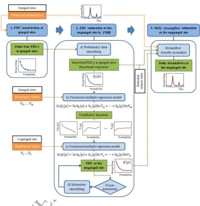
The proposed approach for FDC estimation by FMR, and daily streamflow estimation at ungauged sites comprises three main steps. First, the FDC at each gauged site is constructed from observed daily streamflow series by identifying empirical FDC quantiles at selected percentile points. This results in a point-wise FDC at each gauged site. Second, the FDC at the ungauged site is estimated as a whole by using FMR, for which FDCs from the previous step are represented as functional response inputs (whole curves), and available descriptors as covariates. Decreasing monotonicity of the predicted FDC is assured by monotone smoothing. Third, a transfer procedure is applied to obtain daily streamflow series at the ungauged site. An overview of the procedure is shown in Fig. 1. Steps and the assessment criteria used for evaluating the performance of the proposed approach are further described below.

3.1. FDC at gauged sites

The FDC at each gauged site is built from the corresponding observed daily streamflow series. Specifically, it is obtained by representing the sorted daily streamflow values in the y-axis and their corresponding empirical probability of exceedance in the x-axis. This probability of exceedance (or percentile point p) is usually obtained from the Weibull plotting formula (e.g. Fennessey and Vogel 1990). In order to have a consistent database from all sites, FDC quantiles

ACCEPTED MANUSCRIPT

are identified at a number of fixed percentile points for characterising the FDC. As a result, a set of point-wise FDCs with 17 unevenly spread percentile points are obtained (e.g. Shu and Ouarda 2012).

3.2. Functional multiple regression for FDC estimation

The second step of the proposed FDA-based approach is the FDC estimation at ungauged sites by using FMR (see Fig. 1), which is summarised below:

- The point-wise FDCs at the gauged sites need to be represented as functions to be considered as the functional response in the FMR model. This is done by using preliminary B-Spline smoothing, as indicated in Sect. 2.1;

- Functional FDCs and catchment descriptor values at the gauged sites, such as physiographic or climatic variables, are used to estimate the coefficient functions in the FMR model. Estimated coefficient functions, as well as descriptor values at the ungauged sites are then used to obtain the FDC at the ungauged site. Decreasing monotonicity of the predicted FDC at the ungauged site is ensured by monotone smoothing if this condition is not preserved during the FMR estimation process (Sect. 3.2.1);

- This FMR analysis is performed by considering several practical settings (Sect. 3.2.2).

3.2.1. FDC estimation

The application of FMR to estimate FDCs at ungauged sites, as well as differences between traditional MR and FMR are described below. In traditional MR, the regression equation used for estimating FDCs at ungauged sites is commonly logarithmically transformed into the following linear equation (e.g. Shu and Ouarda 2012):

ACCEPTED MANUSCRIPT

where is the FDC quantile associated with a given percentile point p in at site i and are the k physiographic or climatic descriptors for site i. The coefficients are the model parameters, is the intercept term, and is the residual term. Therefore, as a given p is associated with a given , a regression equation needs to be performed for each p in traditional MR.

Eq. (5) may be expressed as follows when considering FMR:

and (0, 1) (6) where are the FDC quantiles, as functional response, associated with the percentile points p in (0,1) at site i. In other words, they represent the preliminarily smoothed FDCs at the gauged sites. are the k scalar physiographic or climatic descriptors for the site i, the coefficient functions are the model parameters expressed as functions over p; and and are respectively the intercept and the residual term as a function over p. Therefore, only a single regression equation containing all the information needs to be performed in FMR, instead of multiple equations as in MR.

As it can be seen, the structures of Eq. (2) and Eq. (6) are equivalent. The argument t in Eq. (2) corresponds to the percentile point in Eq. (6) for . Thus, the FDA-based approach in this study is not performed over the usual time t but over the percentile point p, which is the probability of exceedance of the FDC quantile. The coefficient functions to be estimated by FMR in Eq. (6) are then expressed hereafter as for each descriptor variable j with . Analogously to traditional MR, the coefficients are assumed to be common for all sites in a region. They are then estimated and used for predicting the whole FDC at the ungauged site, which is done by supplying its catchment descriptor values into Eq. (6). Also note that since the coefficients are functions over p, they may also be used to better understand the effect

ACCEPTED MANUSCRIPT

of each descriptor considered in the regression model over p (see Sect. 4.2.2). Finally, it may happen that the predicted FDC does not fulfil the decreasing monotonicity condition. A common method for assuring monotonicity in FDA is monotone smoothing (Ramsay et al 2009), which is considered in the present study. This is done by explicitly expressing the derivative of the target function as the exponential of a previously estimated B-Spline.

3.2.2. Settings

In the present study, several FMR practical settings are assessed to identify the best one for FDC estimation at ungauged sites. The settings are defined based on two factors: the number of FDC quantiles initially identified at the gauged sites, and the way in which B-Spline functions are defined. Two cases are considered for each factor, leading to four settings A, B, C and D. They are summarised in Table 1 and described below.

FDC quantiles associated with a number of unevenly spread percentile points are usually considered to characterise the whole FDC. In traditional approaches, the number of quantiles is kept small due to the need to perform a regression equation for each quantile. Nevertheless, in FMR, the interest resides in the whole curve and a single regression model is performed. Thus, the use of more FDC quantiles is expected to improve the FDC estimation, while no more complexity is added to the model. Two cases are considered in this regard: the use of 17 percentile points; and the use of a larger number such as 50 percentile points. Note that FDC quantiles are directly obtained from the hydrological information at gauged sites and hence, obtaining 50 instead of 17 points does not entail a drawback.

Order 4 B-Spline functions may be defined by specifying either the number of basis functions or a sequence of knots. Both cases are considered in the present study, leading to “equidistant knots” and “uneven spread knots”, respectively. For the former case, 10 basis

ACCEPTED MANUSCRIPT

functions are considered since the FDC does not generally exhibit strong variations. For the latter case, a given sequence of 14 knots among the 17 percentile points of the traditional approach is selected after a preliminary analysis (i.e. 0.1%, 95% and 99.9% were excluded). This results in a total of 16 basis functions (Ramsay et al. 2014).

3.3. Daily streamflow estimation by a transfer procedure

The transfer procedure commonly used to obtain daily streamflow series at ungauged sites is the nonlinear spatial interpolation technique (e.g. Hughes and Smakhtin 1996). This streamflow transfer procedure is named in different ways over the literature (see e.g. Archfield et al. 2013), and assumes that the probability of exceedance of the streamflow value for a given day is the same at destination and source sites. The destination site corresponds to the target ungauged site, and the source site corresponds to a gauged site selected by a given criterion, which is explained below in this section. The procedure is based on the use of daily streamflow series and FDC at the source site, and predicted FDC at the destination site. Regarding the FDA-based approach, this is then performed by using the smoothed FDC as the FDC at the source site, and the FDC predicted by FMR at the destination site (see Fig. 1).

The transfer procedure for a given day may be summarised as follows:

- First, the streamflow value at the source site is identified through its FDC, and the corresponding percentile point is obtained;

- Second, this percentile point is used in the estimated FDC at the destination site for evaluating the corresponding FDC quantile, which is selected as the streamflow value for the given day.

In the traditional MR approach, logarithmic interpolation is used for obtaining intermediate points of the FDC that are needed during this procedure. Regarding the FMR approach, the

ACCEPTED MANUSCRIPT

second part of the procedure can be directly carried out analytically through Eq. (6), but not the first part. This is due to the fact that FMR builds the functional FDC but not its inverse, hence the percentile point p cannot be directly obtained from the daily streamflow value. To avoid this issue and without loss of generality, logarithmic interpolation is considered in that case. Note that the FDA-based approach, although analytical, constructs functions point-wisely. Thus, FMR has the advantage of considering a much larger number of points, during interpolation, than the traditional MR approach which is only based on 17 points.

According to the literature, it is preferable to use several source sites in the transfer procedure (e.g. Hughes and Smakhtin 1996). Shu and Ouarda (2012) performed a sensitivity analysis to identify the number of source sites and weighted scheme to be considered regarding the present case study. The use of four source sites, identified and weighted based on geographical distance, was found to be the best choice, and is hence also considered in the present study. This implies that for a given day, the streamflow value at the ungauged site is obtained as a weighted average of the streamflow value obtained by applying the transfer procedure by using each source site. For additional procedures to select source sites and weight schemes, see e.g. Archfield and Vogel (2010), Ergen and Kentel (2016) and Patil and Stieglitz (2012).

3.4. Assessment of the approach

The assessment of the proposed approach is evaluated at two stages: first on the estimated FDC, and then on the estimated daily streamflow series. For both stages, the evaluation is based on the commonly used jackknife (or leave-one-out) technique (Nezhad et al. 2010) that consists in performing the estimation at each site without temporarily considering its information in the multi-site transfer procedure. This implies that one site at a time is considered as temporarily

ACCEPTED MANUSCRIPT

“ungauged”. Classical assessment criteria such as NASH, RMSE, RRMSE, BIAS and RBIAS are considered in this study (e.g. Ouarda and Shu 2009).

In particular, FDC estimation performance is evaluated “per site” and “per quantile”. Note that for comparison among approaches, both assessments are carried out on the M percentile points traditionally considered (M = 17). Per quantile mean performance entails obtaining the mean value of the assessment criteria for a given FDC quantile over N sites (N = 109 in the application below), and then calculating its mean value over M quantiles. Per site mean performance entails obtaining the mean value of the assessment criteria for a given site over M quantiles, and then calculating its mean value over N sites. Note that per quantile and per site results are only equivalent for BIAS and RBIAS criteria. Additionally, the number of sites with an initially non-monotonic FDC over the whole estimated curve is also considered as a criterion for per site evaluation. Daily streamflow estimation performance is evaluated per site, as daily streamflow series are estimated at each “ungauged” site.

4. Application

4.1. Case study

The proposed approach is applied to a case study consisting of 109 sites in the hydrometric station network of the province of Quebec, Canada (Fig. 2). Daily streamflow information, as well as physiographical and meteorological descriptors are available at the sites. Selected sites have a minimum period of record of 10 years, through which the FDCs are built at the gauged sites. The mean record length of the set of sites is larger than 25 years. Additional information on the case study can be found in Shu and Ouarda (2012). For coherence and comparison purposes, the same descriptors and transformations as in the aforementioned reference are considered in the present study. Considered descriptors are catchment area (BV), fraction of catchment area

ACCEPTED MANUSCRIPT

controlled by lakes (PLAC), fraction of catchment area occupied by forest (PFOR), catchment mean slope (PMBV), annual mean degree-days below 0°C (DJBZ), annual mean total precipitation (PTMA), summer mean liquid precipitation (PLME), annual mean degree-days over 13°C (DJH13), average number of days with temperature over 27°C (NJH27) and curve number (NCM). If available, additional variables, such as geological or lithological descriptors, could provide useful information when estimating low flows.

4.2. Results

4.2.1. FDC estimation performance

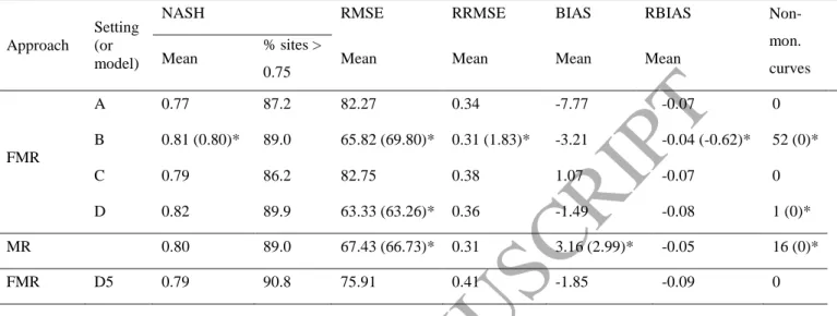
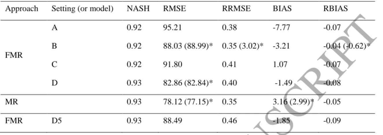
The performance of the four FMR settings (see Table 1) considered for FDC estimation at ungauged sites is evaluated by the assessment criteria in Sect. 3.4. Per site mean performance of the FDC estimation is shown in Table 2. The use of 50 instead of 17 FDC quantiles extracted from the observed daily streamflow series (setting C vs. A, and setting D vs. B) provides better (mean) NASH and BIAS, and (for setting D vs. B) a remarkably lower number of initially non-monotonic predicted FDCs; yet a worse RRMSE. The use of a sequence of unevenly spread instead of equidistant knots for defining B-Splines (setting B vs. A, and setting D vs. C) provides a better NASH, RMSE and RRMSE; yet it increases the number of non-monotonic FDCs especially when fewer FDC quantiles are used. As a result, setting D which consists of 50 FDC quantiles and uneven spread knots may overall be considered as the best setting for per site FDC estimation. This setting obtains the largest NASH and the lowest RMSE among all settings, and only one non-monotonic FDC.

An analogous analysis is carried out on per quantile mean performance of the FDC estimation (Table 3). In this case the use of 50 instead of 17 FDC quantiles (setting C vs. A, and setting D vs. B) leads to a better RMSE and BIAS; yet also a worse RRMSE. The use of a

ACCEPTED MANUSCRIPT

sequence of unevenly spread knots instead of equidistantly distributed knots (setting B vs. A, and setting D vs. C) leads to better RMSE and RRMSE. As a result, setting D may overall be considered as the best setting for per quantile FDC analysis also. In this case, the setting also provides the largest NASH and the lowest RMSE among all settings. Note that extracting a number of FDC points larger than 50 did not lead to relevant per site or per quantile performance improvements.

Per quantile and per site mean FDC results after monotone smoothing on the predicted FDC are shown within parenthesis in Table 2 and Table 3. Recall that monotone smoothing is applied when a predicted FDC does not initially meet the decreasing monotonicity condition. As shown in both tables, FDC estimation performance is affected by the application of monotone smoothing. In some cases, such as for the non-monotonic curve in setting D, the predicted FDC after smoothing is closer to the measured FDC (not shown) and hence, performance results are improved. However, monotone smoothing does not in general allow improving performance results (see setting B results with 52 non-monotonic curves in Table 2 and Table 3). This is due to the fact that the curves that depict a non-monotonicity decrease usually do it at the very beginning or at the very end of the curve, and the effect of monotone smoothing is often large in modifying these curves that were initially almost suitable. This supports the preference for settings that directly provide a low number of non-monotonic FDCs through the FMR model, which is in accordance with the selection of setting D as the best setting for FDC estimation. Note that performing monotone smoothing after the functional estimation process may be seen as a fine-tuning that ensures decreasing monotonicity for all resulting curves. Ensuring decreasing monotonicity is also an issue in traditional MR, where FDC points are estimated separately. For instance, decreasing monotonicity is addressed in Shu and Ouarda (2012) by considering

ACCEPTED MANUSCRIPT

logarithmic interpolation or extrapolation. Note that estimating the extreme points of the FDCs is usually problematic regardless of the approach considered, due to being associated to higher uncertainty than centered points.

Finally, FDC results for the FMR model with setting D are compared with the results obtained by the MR approach proposed in Shu and Ouarda (2012). Results by applying the latter approach are broadly reproduced in the present study to allow comparing intermediate stages in the daily streamflow estimation process, such as the present FDC estimation. Per site mean FDC results (Table 2) are better for the FMR approach (setting D) for NASH, RMSE, BIAS and the number of non-monotonic FDCs; yet worse for RRMSE and RBIAS. This better overall per site performance of the FMR approach may be due to taking into account the fit of all FDC quantiles at the same time. On the other hand, the traditional MR approach obtains better per quantile mean FDC results (Table 3) for RMSE, RRMSE and RBIAS; yet worse for BIAS and the same NASH. This better overall per quantile performance of the traditional MR approach may be due to fitting given FDC quantiles separately, instead of fitting all quantiles at once.

4.2.2. Coefficient functions estimation

The focus of the present section is the estimation of the coefficient functions in Eq. (6). The functional response (left argument in Eq. (6)) is formed by FDCs at gauged sites after preliminary data smoothing. According to the selected setting D (see Table 1), FDCs at gauged sites are formed by 50 quantiles, and B-splines in the smoothing are defined by uneven spread knots. Eq. (6) is built by following a jackknife procedure. This implies that FDCs and catchment descriptor information for all gauged sites, except the site considered as “ungauged”, is used in the regression model. Note that each set of estimated coefficients will be later used for

ACCEPTED MANUSCRIPT

predicting the FDC at the corresponding ungauged site by supplying its descriptor values in Eq. (6).

With the aim of analysing the effect of the descriptors in the FDC estimation for the study region, the estimated coefficients are multiplied by their corresponding descriptor value at the “ungauged” site. For instance, the scaled coefficient function associated to the catchment descriptor BV may be expressed as , where “BV” represents the catchment area at the ungauged site and “ln” shows the logarithmic transformation considered for the descriptor. Scaling allows visually comparing the effect of all descriptors in the FMR model. For this purpose, the 50th point-wise percentile (median) and the 25th-75th point-wise percentile interval (confidence interval) of the scaled values over the 109 sites are displayed regarding the percentile point p in Fig. 3c. Similar scales are considered for facilitating the interpretation of the results. The median provides information about the influence of each descriptor (in general and over p) in FDC estimation; whereas the confidence interval provides information about the variability of the estimated FDC over sites. This analysis is first carried out for all descriptors, and then variable selection is considered based on it.

Catchment area (BV) has the strongest influence on the estimated FDC quantile with respect to all p values, as its median is large and stable over p (see Fig. 3c). The also large and stable confidence interval over p indicates that BV is very important in representing the variability of the estimated FDC over sites. This is consistent with common knowledge about the relevance of this descriptor regarding streamflow size. Different is the case of the catchment mean slope (PMBV), for which the median and confidence interval over p are always close to zero. Thus, PMBV is expected to have a very small influence for the case study. This may be related to the fact that PMBV ranges from 0.19 to 6.95% in the study region, which are small values for

ACCEPTED MANUSCRIPT

implying large differences among catchment responses. Other descriptors, such as PLAC, NJH27, DJH13 and PLME also contribute to FDC estimation, and to characterisation of its variability over sites. However, their effect changes over p. For instance, DJH13 shows less influence for very low p (floods); and PLAC presents more influence for very low (floods) and for moderate to high p (low flows). The FDC variability over sites is less represented by PTMA, DJBZ, PFOR and NCM, where the influence of the latter slightly increases as p increases. Therefore, aside from helping to better understand the behaviour of the descriptors in the regression model, this information could also be useful if additional analyses on a specific range of the FDC need to be performed. This insight cannot be directly obtained from the traditional MR approach.

The median and confidence interval over p are also shown to compare point-wise FDCs obtained from observed daily streamflows and estimated FDCs (after smoothing if needed). As shown in Fig. 3a, results from measured and estimated FDCs are close to each other. Median and confidence interval related to the estimated intercept function after being transformed into streamflow scale ( ), and as obtained by the FMR model (l ) are also plotted in Fig. 3b and Fig. 3c, respectively. In this regard, it is important to note that in a particular FMR model where descriptors are categorised as 0 or 1 (i.e. in FANOVA), the intercept in Eq. (2) is indeed the mean, and then each coefficient is able to clearly show its effect on this mean (e.g. Ramsay et al. 2009). However, in a general FMR model this is not that straight, and as seen in Fig. 3b, the shape of may not be that similar to the one of a plausible monotonic FDC.

If variable selection is considered within the FMR model, by only using the descriptors previously identified as presenting a relevant variability over the study region (i.e. BV, PLAC, NJH27, DJH13 and PLME), the shape of becomes similar to that of a plausible monotonic

ACCEPTED MANUSCRIPT

FDC (Fig. 4b). As seen in Fig. 4c, scaled coefficients experience some changes in comparison to the ones shown in Fig. 3c; yet the previous discussion about their overall influence holds. The median and the confidence interval over p from measured and estimated FDCs are also close to each other (Fig. 4a). Therefore, plots of scaled coefficients are useful to select relevant descriptors in the FMR model. Corresponding per site and per quantile FDC estimation results are shown at the end of Table 2 and Table 3, respectively. Note that the model using all descriptors is referred to as FMR-D, and the model using five descriptors is referred to as FMR-D5. As expected, FMR-D results for which more information is used are overall better than FMR-D5 results. Nevertheless, the FMR-D5 model is more appropriate, entails estimating fewer coefficients , and directly obtains monotonically decreasing FDCs at all sites. Previous discussion about comparison of FMR and MR results also holds for FMR-D5, with the exception of FMR-D5 obtaining worse per site mean NASH and RMSE than MR. Note that the MR approach considers all descriptors.

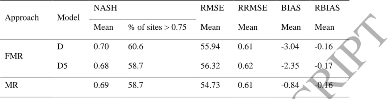
4.2.3. Daily streamflow estimation performance

Assessment criteria results of daily streamflow estimation for FMR by using all (FMR-D) or five descriptors (FMR-D5), as well as for traditional MR are shown in Table 4. Note that results from the latter approach do not exactly correspond with the ones shown in Shu and Ouarda (2012). They are broadly reproduced in this study to allow comparing intermediate stages of the daily streamflow estimation process, such as the FDC estimation; and a 30-year study period from 1971 to 2000 is considered for daily streamflow estimation. As seen in Table 4, overall results for both MR and FMR approaches are very similar. In particular, FMR-D obtained the largest NASH, both FMR-D and MR provided the smallest RRMSE and RBIAS, and MR

ACCEPTED MANUSCRIPT

obtained the smallest RMSE and BIAS. Recall that FMR-D5 only uses five descriptors, whereas FMR-D and MR uses all of them.

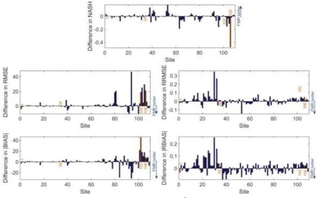
Given the similarity in the obtained daily streamflow results, a deeper at-site analysis is carried out to further explore the behaviour of the various approaches. For this purpose, the difference in performance results for daily streamflow estimation between FMR and MR is computed. Absolute instead of regular at-site BIAS and RBIAS are obtained to allow identifying the approach leading to best results. An overall better behaviour of FMR-D in comparison to the one of MR is found. FMR-D performs better in 58, 58, 51, 46 and 53% of the sites for NASH, RMSE, RRMSE, |BIAS| and |RBIAS|, respectively. Results regarding FMR-D5 are in general less impressive, with the exception of an improvement in |BIAS|. In this case, FMR-D5 performs better than MR in 45, 45, 38, 50 and 45% of the sites for NASH, RMSE, RRMSE, |BIAS| and |RBIAS|, respectively.

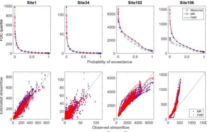
As illustration, the difference in daily streamflow assessment criteria results between FMR-D5 and MR is shown in Fig. 5. After examining the obtained results, several sites (sites 1, 34, 102 and 106) identified as representative of different behaviours are further analysed for illustrative purposes. Measured and estimated FDCs, as well as a scatter plot of observed and estimated daily streamflow values are also shown for these sites in Fig. 6. The flexibility of FMR to build monotonic decreasing FDCs with different shapes may be seen in the figure. Note that the streamflow for a given day is not shown when either its observed or estimated value is unavailable. Also note that estimated daily streamflows may not reach the largest values shown through the associated estimated FDC (Fig. 6), since these events may not happen over the study period for daily streamflow estimation. Assessment criteria results for FDC and daily streamflow estimation for these sites are displayed in Fig. 7.

ACCEPTED MANUSCRIPT

Site 1 is identified as a regular site. It does not entail large differences between approaches (Fig. 5); and its FDC and daily streamflow estimations may be considered as suitable based on graphical and assessment criteria results (see Fig. 6 and 7). FMR-D5 presents an overall better performance for this site. Site 106 has large differences in several assessment criteria results such as in NASH and RMSE (Fig. 5); yet it presents bad FDC and daily streamflow results for both approaches due to a large overestimation of the FDC in both cases (Fig. 6 and 7). The latter may be related to the fact that this site has a large catchment area, which is expected to be associated with larger observed daily streamflows than the ones measured at the site. Thus, as both approaches are regression-based models, they fail to provide a suitable FDC estimation for this site. Note that regression-based models usually obtain better results at moderate sites. On the other side, site 102 with the largest catchment area in the region is better estimated thanks also to having the largest daily streamflows (Fig. 6 and 7). MR provides the best performance in this case, obtaining for both approaches high NASH and small RRMSE and RBIAS. The large RMSE and BIAS of site 102 is due to its large daily streamflow values (Fig. 6 and 7). The case of site 34 is quite different: its large RRMSE may be related to its small daily streamflow values (Fig. 6 and 7). The performance of the approaches for this site depends on the assessment criteria considered.

5. Discussion

The advantage of the MR approach for FDC estimation is the use of simple regression models; yet it implies estimating each FDC quantile separately which is not conceptually appropriate. Therefore, its use may be preferable if only few quantiles are of interest for a given region. This is also supported by per quantile FDC estimation performance results in Table 3. The benefit of the FMR approach resides in the use of a flexible and conceptually supported

ACCEPTED MANUSCRIPT

framework that allows estimating all FDC quantiles jointly. Although FMR requires more complex statistical tools, it also has the advantage of providing information about the influence evolution of the descriptors over the percentile points in the FDC. The use of FMR may then be recommended if a large number of FDC quantiles is of interest for a given region, and if “per site” analysis is the focus, which is supported by per site results in Table 2. This is the focus when daily streamflow series are estimated at ungauged sites, and hence FMR would be more appropriate in such a case. Indeed, although similar mean daily streamflow estimation performance is obtained by FMR and MR for the case study (see Table 4), FMR is able to provide a better performance for a larger percentage of sites.

Among the considered descriptors, catchment area (BV), fraction of catchment area controlled by lakes (PLAC), average number of days with temperature over 27°C (NJH27), annual mean degree-days over 13°C (DJH13) and summer mean liquid precipitation (PLME) were found as relevant catchment descriptors for representing the variability of FDCs over the study region. Their influence may vary over the FDC (Fig. 4c). For instance, floods (low p values) would be more influenced by BV, PLAC and PLME; whereas low flows (high p values) would be more influenced by BV, PLAC, DJH13 and PLME. Through the application of the proposed FMR approach, the practitioner is provided with both the FDC and the daily streamflow series at the target ungauged site. This information may be used in a number of applications, such as water supply planning, hydropower generation or flood protection.

As a regression-based model, the present FMR approach has the limitation of often obtaining better results at moderate sites in terms of range of values of considered descriptors, especially regarding BV. This limitation can be seen through the bad results obtained for site 106 that is associated to a large BV but not very large observed daily streamflows (Fig. 6). The estimation

ACCEPTED MANUSCRIPT

of FDCs at ungauged sites is done by considering the information of all gauged stations in the study area, as also considered in.Shu and Ouarda (2012). However, it should be noted that the selection of a subset of gauged sites based on similarity measures and homogeneity could improve the obtained results (e.g. Castellarin et al. 2004; Mendicino and Senatore 2013; Requena et al. 2017).

Future research could be related to a wider assessment of the benefits and performance of the present approach. This could be done by the application of the approach to a number of case studies, as well as by the comparison of its results with those obtained by different statistical or parametric approaches over the literature. In this regard, it would be relevant to evaluate the performance of the approach when considering intermittent regimes (e.g. Mendicino and Senatore 2013). Further research regarding the improvement of the proposed FMR approach could be related to variable selection, which is an emerging topic in FDA (e.g. Brockhaus et al. 2015; Mingotti et al. 2013). In the present study, this is done through scaled coefficient function plots due to the multi-site transfer context of the analysis. Additional statistical tools for improving FMR results could entail, for instance, the use of functional principal component analysis for defining new variables as combination of existing variables (e.g. Chebana et al. 2012).

Future research should also explore the impact of adopting the FMR approach on the performance of the Regional Streamflow Estimation Based Frequency analysis (RSBFA) approach, recently proposed by Ouarda (2016) and developed by Requena et al. (2017). RSBFA is an approach for regional frequency analysis at ungauged sites. It is based on the regional estimation of daily streamflow series at the ungauged site, through an FDC procedure, and then the estimation of desired quantiles through local frequency analysis. Finally, it would be

ACCEPTED MANUSCRIPT

important to evaluate the performance of a FMR based RSBFA procedure as a simple approach to combine local and regional information in the case of partially gauged sites, in opposition to complex Bayesian statistical models (e.g. Seidou et al. 2006). This analysis will provide information about the real merits and potential of this approach.

6. Conclusions

Flow duration curve (FDC) estimation is often needed to obtain daily streamflow series at ungauged sites. In the present study, given the functional nature of FDC as curves, functional multiple regression (FMR) is proposed for FDC estimation at ungauged sites. Daily streamflow series based on such a FDC estimation are then obtained through a well-known transfer procedure.

Better per site FDC estimation performance is found for the FMR approach; whereas better per quantile FDC estimation performance is found for a traditional multiple regression (MR) approach. Mean daily streamflow estimation performance of both approaches is found to be similar; yet the FMR approach is able to provide a better performance for a larger percentage of sites when considering all the available descriptors. Furthermore, the FMR approach has conceptual and practical advantages, such as the use of a flexible framework for a proper estimation of the whole FDC. This is done by jointly estimating all the FDC quantiles through a single regression model, instead of by building several separate regression equations according to the number of FDC quantiles as in traditional MR. Moreover, the FMR approach provides relevant insight into the influence of the considered descriptors within the overall regression model, as well as over the FDC quantiles. Note that the latter cannot be directly obtain by traditional methods. For the case study in the province of Quebec, Canada, it was found that among the considered descriptors, catchment area (BV), fraction of catchment area controlled by

ACCEPTED MANUSCRIPT

lakes (PLAC), average number of days with temperature over 27°C (NJH27), annual mean degree-days over 13°C (DJH13) and summer mean liquid precipitation (PLME) were relevant in representing FDCs over the region. Their influence changes over the FDC.

While the traditional MR approach may be of interest if the focus is the estimation of few FDC quantiles in a region, the FMR approach would be more appropriate if the focus is a large number of FDC quantiles or the whole FDC for a given site, and hence to daily streamflow estimation at ungauged sites. In the same line as traditional methods, FDC and daily streamflow series may be obtained at the target ungauged site through the application of the proposed FMR approach to be used in water supply planning or flood assessment activities, among others.

Acknowledgements

The financial support provided by the Natural Sciences and Engineering Research Council of Canada (NSERC), and the Merit scholarship program for foreign students - Postdoctoral research fellowship of the Fonds de recherche du Québec – Nature et technologies (FRQNT) is gratefully acknowledged. The authors would like to acknowledge the assistance from Thi Mui Pham. The authors would also like to thank the Editor, Associated Editor and two anonymous reviewers whose comments helped improve the present paper.

Abbreviation list

Abbreviation Definition

FDA Functional data analysis FDC Flow duration curve

MR Multiple regression

FMR Functional multiple regression FANOVA Functional analysis of variance

ACCEPTED MANUSCRIPT

Adham, M. I., Shirazi, S. M., Othman, F., Rahman, S., Yusop, Z., Ismail, Z. 2014. Runoff potentiality of a watershed through SCS and functional data analysis technique. The Scientific World Journal. 2014, 15pp.

Archfield, S.A., Vogel, R.M., 2010. Map correlation method: Selection of a reference streamgage to estimate daily streamflow at ungaged catchments. Water Resour. Res. 46(10), W10513.

Archfield, S.A., Steeves, P.A., Guthrie, J.D., Ries III, K.G., 2013. Towards a publicly available, map-based regional software tool to estimate unregulated daily streamflow at ungauged rivers. Geoscientific Model Development. 6, 101-115.

Brockhaus, S., Scheipl, F., Hothorn, T., Greven, S., 2015. The functional linear array model. Statistical Modelling. 15(3), 279-300.

Brumback, B.A., Rice, J.A., 1998. Smoothing spline models for the analysis of nested and crossed samples of curves. J. Am. Stat. Assoc. 93(443), 961-976.

Castellarin, A., Galeati, G., Brandimarte, L., Montanari, A., Brath, A., 2004. Regional flow-duration curves: reliability for ungauged basins. Adv. Water Resour. 27, 953-965.

Castellarin, A., Camorani, G., Brath, A., 2007. Predicting annual and long-term flow-duration curves in ungauged basins. Adv. Water Resour. 30, 937-953.

Castellarin, A., Botter, G., Hughes, D.A., Liu, S., Ouarda, T.B.M.J., Parajka, J., Post, D.A., Sivapalan, M., Spence, C., Viglione, A., Vogel, R.M., 2013. Prediction of flow duration curves in ungauged basins, in “Runoff Prediction in Ungauged Basins: Synthesis across Processes, Places and Scales”, edited by G. Bloschl et al., University Press, Cambridge. 135-162.

ACCEPTED MANUSCRIPT

Chebana, F., Dabo-Niang, S., Ouarda, T.B.M.J., 2012. Exploratory functional flood frequency analysis and outlier detection. Water Resour. Res. 48(4), W04514.

Ergen, K., Kentel, E., 2016. An integrated map correlation method and multiple-source sites drainage-area ratio method for estimating streamflows at ungauged catchments: A case study of the Western Black Sea Region, Turkey. J. Environ. Manage. 166, 309-320.

Faraway, J.J., 1997. Regression analysis for a functional response. Technometrics. 39(3), 254-261.

Fennessey, N., Vogel, R.M., 1990. Regional flow-duration curves for ungauged sites in Massachusetts. J. Water Resour. Plann. Manage. 116, 530-549.

Hughes, D., Smakhtin, V., 1996. Daily flow time series patching or extension: a spatial interpolation approach based on flow duration curves. Hydrological Sciences Journal. 41, 851-871.

Li, M., Shao, Q., Zhang, L., Chiew, F.H., 2010. A new regionalization approach and its application to predict flow duration curve in ungauged basins. Journal of Hydrology. 389, 137-145.

Masselot, P., Dabo-Niang, S., Chebana, F., Ouarda, T.B.M.J., 2016. Streamflow forecasting using functional regression. Journal of hydrology. 538, 754-766.

Mendicino, G., Senatore, A., 2013. Evaluation of parametric and statistical approaches for the regionalization of flow duration curves in intermittent regimes. Journal of hydrology. 480, 19-32.

Mingotti, N., Lillo, R.E., Romo, J., 2013. Lasso variable selection in functional regression. Statistics and Econometrics Series 13. Working paper 13-14.

ACCEPTED MANUSCRIPT

Mohamoud, Y.M., 2008. Prediction of daily flow duration curves and streamflow for ungauged catchments using regional flow duration curves. Hydrological Sciences Journal. 53, 706-724.

Nezhad, M.K., Chokmani, K., Ouarda, T.B.M.J., Barbet, M., Bruneau, P., 2010. Regional flood frequency analysis using residual kriging in physiographical space. Hydrological Processes. 24(15), 2045-2055,

Ouarda, T.B.M.J., Shu, C., 2009. Regional low-flow frequency analysis using single and ensemble artificial neural networks. Water Resour. Res. 45, W11428.

Ouarda, T.B.M.J., 2016. Regional Flood Frequency Modeling. Chapter 77. In Handbook of Applied Hydrology (V.P. Singh, Editor). McGraw-Hill, New York.

Patil, S., Stieglitz, M., 2012. Controls on hydrologic similarity: role of nearby gauged catchments for prediction at an ungauged catchment. Hydrology and Earth System Sciences. 16, 551-562.

Ramsay, J.O., 1982. When the data are functions. Psychometrika. 47(4), 379-396. Ramsay, J.O., Silverman B., 2005. Functional data analysis. Springer.

Ramsay, J.O., Hooker, G., Graves, S., 2009. Functional data analysis with R and MATLAB. Springer.

Ramsay, J.O., Wickham, H., Graves, S., Hooker, G., 2014. fda: Functional Data Analysis. R package version 2.4.4. https://CRAN.R-project.org/package=fda

Requena, A.I., Ouarda, T.B.M.J., Chebana, F., 2017. Flood frequency analysis at ungauged sites based on regionally estimated streamflows. Journal of Hydrometeorology, 18(9), 2521-2539.

ACCEPTED MANUSCRIPT

Requena, A.I., Chebana, F., Ouarda, T.B.M.J., 2017. Heterogeneity measures in hydrological frequency analysis: review and new developments. Hydrology and Earth System Sciences, 21, 1651-1668.

Seidou, O., Ouarda, T.B.M.J., Barbet, M., Bruneau, P., Bobée, B., 2006. A parametric Bayesian combination of local and regional information in flood frequency analysis. Water Resour. Res. 42, W11408.

Shu, C., Ouarda, T.B.M.J., 2012. Improved methods for daily streamflow estimates at ungauged sites. Water Resour. Res. 48, W02523.

Smakhtin, V., Hughes, D., Creuse-Naudin, E., 1997. Regionalization of daily flow characteristics in part of the Eastern Cape, South Africa. Hydrological Sciences Journal. 42, 919-936. Ssegane, H., Amatya, D.M., Tollner, E., Dai, Z., Nettles, J.E., 2013. Estimation of daily

streamflow of southeastern coastal plain watersheds by combining estimated magnitude and sequence. Journal of the American Water Resources Association. 49, 1150-1166.

Stone, M., 1974. Cross-validatory choice and assessment of statistical predictions. J. Roy. Stat. Soc. Ser. B (Methodol.), 111-147.

Ternynck, C., Ben Alaya, M.A., Chebana, F., Dabo-Niang, S., Ouarda, T.B.M.J., 2016. Streamflow hydrograph classification using functional data analysis. Journal of hydrometeorology. 17(1), 327-344.

Zhang, Y., Vaze, J., Chiew, F.H., Li, M., 2015. Comparing flow duration curve and rainfall– runoff modelling for predicting daily runoff in ungauged catchments. Journal of Hydrology. 525, 72-86.

ACCEPTED MANUSCRIPT

Table 1. Functional multiple regression settings.

Setting No. of FDC quantiles at

gauged sites Percentile points (%) B-Splines

A 17 0.01, 0.1, 0.5, 1, 5, 10, 20, 30, 40, 50, 60, 70, 80, 90, 95, 99, 99.99.

Equidistant knots

B 17 Uneven spread knots

C 50 0.01, 0.05, 0.1, 0.3, 0.5, 0.7, 1, 3, 5, 7, 10, 13, 15, 17, 20, 23, 25, 27, 30, 33, 35, 37, 40, 43, 45 ,47, 50, 53, 55, 57, 60, 63, 65, 67, 70, 73, 75, 77, 80, 83, 85, 87, 90, 93, 95, 97, 99, 99.5, 99.9, 99.99 Equidistant knots

ACCEPTED MANUSCRIPT

Table 2. Per site assessment criteria results of FDC estimation by a jackknife procedure.

Approach

Setting (or model)

NASH RMSE RRMSE BIAS RBIAS

Non-mon. curves Mean % sites >

0.75 Mean Mean Mean Mean

FMR A 0.77 87.2 82.27 0.34 -7.77 -0.07 0 B 0.81 (0.80)* 89.0 65.82 (69.80)* 0.31 (1.83)* -3.21 -0.04 (-0.62)* 52 (0)* C 0.79 86.2 82.75 0.38 1.07 -0.07 0 D 0.82 89.9 63.33 (63.26)* 0.36 -1.49 -0.08 1 (0)* MR 0.80 89.0 67.43 (66.73)* 0.31 3.16 (2.99)* -0.05 16 (0)* FMR D5 0.79 90.8 75.91 0.41 -1.85 -0.09 0

*(.) Smoothed results are shown within parenthesis if non-monotonic FDCs are initially obtained, and if smoothed and unsmoothed results present differences by considering two decimals.

FMR settings A, B, C and D are described in Table 1. Model FMR-D5 corresponds with setting D by using five instead of all descriptors. MR refers to traditional multiple regression.

ACCEPTED MANUSCRIPT

Table 3. Per quantile mean assessment criteria results of FDC estimation by a jackknife procedure.

Approach Setting (or model) NASH RMSE RRMSE BIAS RBIAS

FMR A 0.92 95.21 0.38 -7.77 -0.07 B 0.92 88.03 (88.99)* 0.35 (3.02)* -3.21 -0.04 (-0.62)* C 0.92 91.80 0.41 1.07 -0.07 D 0.93 82.86 (82.84)* 0.40 -1.49 -0.08 MR 0.93 78.12 (77.15)* 0.35 3.16 (2.99)* -0.05 FMR D5 0.93 88.49 0.46 -1.85 -0.09

*(.) Smoothed results are shown within parenthesis if non-monotonic FDCs are initially obtained, and if smoothed and unsmoothed results present differences by considering two decimals.

FMR settings A, B, C and D are described in Table 1. Model FMR-D5 corresponds with setting D by using five instead of all descriptors. MR refers to traditional multiple regression.

ACCEPTED MANUSCRIPT

Table 4. Assessment criteria results of daily streamflow estimation.

Approach Model

NASH RMSE RRMSE BIAS RBIAS

Mean % of sites > 0.75 Mean Mean Mean Mean

FMR

D 0.70 60.6 55.94 0.61 -3.04 -0.16

D5 0.68 58.7 56.32 0.62 -2.35 -0.17

MR 0.69 58.7 54.73 0.61 -0.84 -0.16

Model FMR-D corresponds with setting D as described in Table 1. Model FMR-D5 entails using five instead of all descriptors. MR refers to traditional multiple regression.

ACCEPTED MANUSCRIPT

Fig. 1 Overview of the proposed procedure for FDC estimation by using functional multiple regression, and daily streamflow estimation at ungauged sites.

ACCEPTED MANUSCRIPT

ACCEPTED MANUSCRIPT

Fig. 3 Functional multiple regression results for model (or setting) D displayed by the median and [25th-75th] confidence interval over 109 sites regarding p: (a) measured vs. estimated

point-wise FDC; (b) intercept function in streamflow scale; (c) intercept function, and 10 coefficient functions scaled by their descriptor value.

ACCEPTED MANUSCRIPT

Fig. 4 Functional multiple regression results for model D5 displayed by the median and [25th-75th] confidence interval over 109 sites regarding p: (a) measured vs. estimated point-wise FDC;

(b) intercept function in streamflow scale; (c) intercept function, and five coefficient functions scaled by their descriptor value.

ACCEPTED MANUSCRIPT

Fig. 5 Difference in daily streamflow assessment criteria results between multiple regression and functional multiple regression (model D5). Marked sites are further analysed.

ACCEPTED MANUSCRIPT

Fig. 6 Measured and estimated FDC (top), and daily streamflows (bottom) at several sites for multiple regression and functional multiple regression (model D5).

ACCEPTED MANUSCRIPT

Fig. 7 Assessment criteria results of FDC and daily streamflow estimation at several sites for multiple regression and functional multiple regression (model D5).