HAL Id: tel-02482710
https://pastel.archives-ouvertes.fr/tel-02482710
Submitted on 18 Feb 2020
HAL is a multi-disciplinary open access archive for the deposit and dissemination of sci-entific research documents, whether they are pub-lished or not. The documents may come from teaching and research institutions in France or abroad, or from public or private research centers.
L’archive ouverte pluridisciplinaire HAL, est destinée au dépôt et à la diffusion de documents scientifiques de niveau recherche, publiés ou non, émanant des établissements d’enseignement et de recherche français ou étrangers, des laboratoires publics ou privés.
Haitao Tian
To cite this version:
Haitao Tian. Taylor meshless method for thin plates. Other [cond-mat.other]. Ecole nationale supérieure d’arts et métiers - ENSAM, 2019. English. �NNT : 2019ENAM0036�. �tel-02482710�
Arts et Métiers ParisTech - Campus de Metz
Laboratoire d’Étude des Microstructures et de Mécanique des Matériaux (LEM3) UMR CNRS 7239
T
H
È
S
E
2019-ENAM-0036École doctorale n° 432 : Science des Métiers de l’ingénieur
Doctorat
T H È S E
pour obtenir le grade de docteur délivré par
l’École Nationale Supérieure d'Arts et Métiers
Spécialité “ Mécanique - matériaux ”
présentée et soutenue publiquement par
Haitao TIAN
le 06 décembre 2019
Taylor Meshless Method for Thin Plates
Directeur de thèse : Farid ABED-MERAIM Co-encadrement de la thèse : Michel POTIER-FERRY
Jury
M. Hamid ZAHROUNI,Professeur, Université de Lorraine, France Président
M. Fan XU,Professeur, Fudan University, Shanghai, China Rapporteur
M. Noureddine DAMIL,Professeur, Université Hassan II de Casablanca, Maroc Rapporteur
M. Yao KOUTSAWA,Chercheur (HDR), LIST, Luxembourg Examinateur
M. Farid ABED-MERAIM,Professeur, Arts et Métiers, France Examinateur
Acknowledgments
I would like to express my sincere appreciation to my supervisor Professor Michel POTIER-FERRY for his great patience and continuous guidance on my PhD study. His immense knowledge and support light up my research career in difficult days. I deeply thank my supervisor Professor Farid ABED-MERAIM for his responsible supervision and valuable suggestions and encouragement. Without his guidance and persistent help this dissertation would not have been possible.
Many thanks to the organization China Scholarship Council (CSC). The funding from my country supports my study and living in France.
I really appreciate the help from my colleagues Peng WANG, Jie YANG, Hocine CHALAL, Mohamed BEN BETTAIEB, Holanyo Koffi AKPAMA, etc. I also thank my Chinese friends for the memorable days we have had together in the past few years.
Last but not the least, I would like to express my gratitude to my parents and my girlfriend for their sacrifices and spiritual support. The encouragement from them is the strength that sustains me thus far.
Contents
Contents ... i
List of Tables and Figures ...iii
Chapter 1 Literature review on meshless methods ... 1
1.1 Research background ... 1
1.1.1 Finite difference method ... 2
1.1.2 Finite element method ... 3
1.1.3 Boundary element method ... 5
1.2 Meshless methods ... 5
1.2.1 Approximation approaches of field functions ... 6
1.2.2 Galerkin formulation and collocation formulation ... 10
1.2.3 Taylor Meshless Method ... 14
1.3 Organization of the thesis ... 15
Chapter 2 Techniques of Taylor Meshless Method ... 17
2.1 Introduction ... 17
2.2 Resolution of partial differential equations ... 17
2.3 Treatment of boundary and interface conditions ... 20
2.4 Application to 2D Laplace equation ... 22
2.5 Application of TMM to Kirchhoff plate problems ... 24
2.5.1 Calculation of the shape functions ... 25
2.5.2 Kirchhoff plate problem with a circular domain ... 29
2.5.3 Kirchhoff plate problem with a rectangular domain ... 31
2.6 Application of TMM to sandwich plates... 35
2.6.1 The loading and the governing equation ... 35
2.6.2 Exact solution ... 35
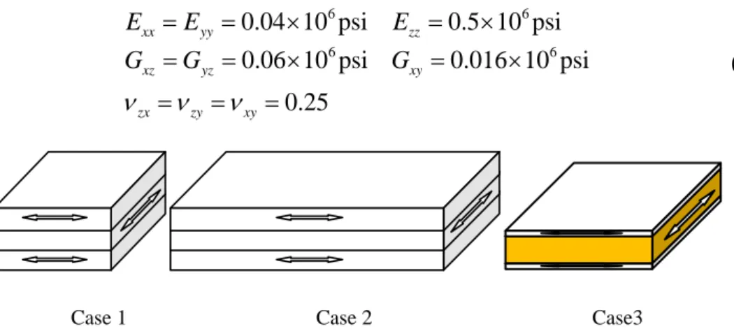
2.6.3 The properties of each case ... 35
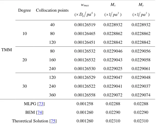
2.6.4 Results ... 37
ii
Chapter 3 Application of TMM to large deflection of thin plates ... 42
3.1 Introduction ... 42
3.2 Governing equations ... 44
3.3 Combination of TMM and ANM ... 45
3.3.1 The procedure of ANM ... 45
3.3.2 TMM formulation ... 48
1.1.1 Treatment of boundary and interface conditions ... 50
3.4 Results and discussion ... 54
3.4.1 Buckling of a square plate with movable edges ... 55
3.4.2 Bending of a square plate with immovable edges ... 57
3.4.3 Buckling of a square plate with immovable edges under uniaxial compression ... 59
3.5 Conclusion ... 63
Chapter 4 Application of TMM to wrinkling of membranes under shear loading ... 64
4.1 Introduction ... 64
4.2 Modelling of the membrane boundary value problem ... 65
4.3 Numerical Results ... 69
4.3.1 Generation of membrane wrinkles ... 69
4.3.2 Sensitivity with respect to the number of subdomains ... 71
4.3.3 Sensitivity with respect to tension loads ... 72
4.3.4 Imperfection sensitivity ... 79
4.4 Conclusion ... 80
Conclusions and future works ... 82
References ... 84
List of Tables and Figures
Table 2.1 Organization of the computation ... 28
Table 2.2 Deflection and moment of the center of a rectangular plate, clamped edges, uniform load ... 34
Table 3.1 Deflection and membrane stress at the center of plate vs. load p ... 58
Table 3.2 Displacement load values when the displacement of center pointw 1, convergence with mesh refinement and with the degree ... 62
Table 4.1 Material property ... 67
Table 4.2 Sensitivity of the response (number of wrinkles) to the number of sub-domains. Pre-tension v 0.02mm, imperfection 0.001mm. ... 72
Table 4.3 Number of wrinkles with different tension loads. ... 73
Table 4.4 The maximum displacements and amplitudes of center wrinkles, shear load 0.15mm, imperfection 0.001mm. ... 74
Table 4.5 Sensitivity of the response (number of wrinkles) to the imperfection. Pre-tension v 0.02mm, number of sub-domains: 33×11. ... 80
Figure 1.1 The procedure of scientific computation ... 1
Figure 1.2 The cover of the domain by kernel functions ... 7
Figure 1.3 Background grid of EFGM for integration ... 12
Figure 1.4 Domains and boundaries in MLPG ... 13
Figure 2.1 One domain with Dirichlet and Neumann boundary conditions ... 20
Figure 2.2 Multidomains and the interface ... 21
Figure 2.3 Distribution of collocation points ... 23
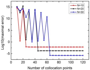
Figure 2.4 The influence of the number of collocation points for Eq.(2.25), N=10, 20, 30 ... 24
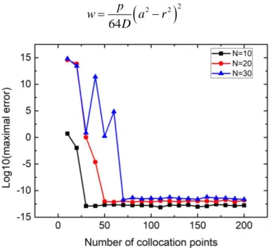
Figure 2.5 The influence of the degree N for Eq.(2.25),M 4N ... 24
Figure 2.6 A circular Kirchhoff plate with clamped edges ... 29
Figure 2.7 The influence of the number of collocation points on the convergence for circular Kirchhoff plate ... 30
iv
Figure 2.8 The convergence of TMM for circular Kirchhoff plate ... 31
Figure 2.9 Rectangular domain and collocation points on the boundaries ... 31
Figure 2.10 The distribution of the deflection from Eq.(2.42) ... 32
Figure 2.11 The influence of the number of collocation points on the convergence for rectangular Kirchhoff plate ... 33
Figure 2.12 The convergence of TMM for rectangular Kirchhoff plate ... 33
Figure 2.13 The distribution of the deflection of a clamped Kirchhoff plate ... 34
Figure 2.14 Fiber directions and thickness of each case ... 37
Figure 2.15 The coordinate system and expansion point ... 37
Figure 2.16 The influence of the degree on the convergence, Case1 ... 38
Figure 2.17 The influence of the number of collocation points on the convergence, N = 16, Case1 ... 38
Figure 2.18 The influence of the degree on the convergence, Case2 ... 39
Figure 2.19 The influence of the number of collocation points on the convergence, N = 16, Case2 ... 39
Figure 2.20 The influence of the degree on the convergence, Case3 ... 40
Figure 2.21 The influence of the number of collocation points on the convergence, N = 16, Case3 ... 40
Figure 2.22 The influence of expand point on the convergence ... 41
Figure 3.1 A square and simply supported plate with boundary collocation points 50 Figure 3.2 A square plate with immovable edges ... 51
Figure 3.3 Effect of small perturbations on the buckling of a simply supported square plate. The ANM-TMM algorithm is compared with a commercial finite element code. On the ANM-TMM curve, each point corresponds to one ANM step ... 55
Figure 3.4 A zoom of Figure 3.3. One sees that the ANM-TMM method permits to compute easily quasi-perfect bifurcations. On the ANM-TMM curve, each point corresponds to one ANM step. ... 56
Figure 3.5 h-convergence: decimal logarithm of the error on the bifurcation stress, according to the degreePand to the number of subdomains. ... 56
Figure 3.6 Deflection at the center of plate vs. load p ... 57
Figure 3.7 A square plate with immovable edges ... 59
Figure 3.8 Displacement of center point of the plate vs. load, degree of TMM 8, order of ANM 10 ... 60
Figure 3.9 The deformation of the plate at point A, B, C, D in Figure 3.8 ... 60
Figure 3.10 Comparison of results by FEM and TMM with degree 8 and 10 ... 61
Figure 3.11 The deformation of the plate at point E in Figure 3.10 ... 61
Figure 3.12 Displacement load values when the displacement of center point is 1 ... 62
Figure 4.1 Rectangular membrane with tensionvand shear loadu ... 67
Figure 4.2 Steps of the algorithm ... 67
Figure 4.3 An imperfection sample ... 68
Figure 4.4 Imperfection of the membrane for wrinkling, tension load 0.02mm, imperfection 0.001mm. ... 70
Figure 4.5 Full wrinkled membrane, 33×11 domains, tension load 0.02mm, imperfection 0.001mm. ... 70
Figure 4.6 Full wrinkled membrane. Subdomains: 21×11, tension load 0.02mm, imperfection 0.001mm, shear load 0.15mm. ... 72
Figure 4.7 Wrinkle patterns with different tension loads. ... 73
Figure 4.8 Shear load vs maximum displacement, tension loads from 0.0005mm to 0.08mm, imperfection 0.001mm. ... 74
Figure 4.9 A zoom of the buckling curve, tension load 0.05mm. ... 75
Figure 4.10 Deformations of the membrane with different shear loads, tension load 0.05mm. ... 76
Figure 4.11 A zoom of the buckling curve, tension load 0.001mm. ... 77
Figure 4.12 Deformations of the membrane with different shear loads, tension load 0.001mm. ... 77
Figure 4.13 A zoom of the buckling curve, tension load 0.0005mm. ... 78
Figure 4.14 Deformations of the membrane with different shear loads, tension load 0.0005mm. ... 79
Chapter 1 Literature review on meshless
methods
1.1 Research background
Numerical simulation on computers has become an important tool to study and predict the behavior of physical systems, especially for those who cannot provide analytical solutions, as in most nonlinear systems [1]. The procedure of scientific computation and solving technical problems consists of several steps, as shown in Figure 1.1. Practical problem Mathematical model Numerical method Programme design Computation Solution
Figure 1.1 The procedure of scientific computation
The premise and basis of scientific computation is modeling practical problems based on scientific theory, mathematical theory and some reasonable assumptions. However, the key of the procedure is to obtain solutions of mathematical models which can meet accuracy requirements using computers. This is a new branch of mathematics - Numerical Analysis, including function interpolation, numerical differentiation and integration, solving systems of linear and nonlinear equations, calculation of matrix eigenvalues and eigenvectors, computational methods for optimization problems, numerical solutions of ordinary differential equations and partial differential equations, etc. It also involves theoretical research on reliability of computational methods, such as convergence, stability and error estimation.
Numerical analysis is applied widely in fundamental industrial production and researches of the most advanced science and technology. It provides an alternative way of scientific investigation besides theoretical solutions and expensive,
2
time-consuming experiments, becoming essential in optimization design of mechanical and electrical products, geological exploration and oilfield development, weather forecast and earthquake prediction, development of cutting-edge weapons and aerospace. Furthermore, it has infiltrated into different science fields, generating interdisciplinary subjects such as computational physics, digital image processing and econometrics.
On this background, computational mechanics is formed by the interdisciplinary of numerical analysis and mechanics, which deals with the use of computational methods in engineering practices to study physical phenomena governed by the principles of mechanics [2]. Over the past few decades, it has shown huge potential for the application on physical and biological systems based on classical mechanics, quantum mechanics and biology. The computational mechanics are extended to the areas of mechanics, mathematics, computer science, making a significant contribution in the design and simulation of new products because of the advantages of convenience, effectiveness and high efficiency. The computational method has become one of the most important tools in engineering and science, covering various topics including thermal, fluid, solid mechanics, vibration, and vehicle dynamics.
Among numerous computational methods in computational mechanics, the most popular ones are finite difference methods (FDM), finite element methods (FEM) and boundary element methods (BEM). They are widely used for solving engineering problems, especially finite element methods. However, despite of widespread applications, they have their own shortcomings and limitations. The advantages and disadvantages of these methods are introduced and detailed in this section.
1.1.1 Finite difference method
The finite difference methods (FDM) is one of the most traditional and simplest methods for solving differential equations by approximating them with difference equations, in which finite differences approximate the derivatives [3].
FDM solves the original linear or nonlinear differential equations by converting them into a linear system, which can be solved by matrix techniques. The finite difference approximation began to develop rapidly with the widespread use of computers. The accuracy, stability and convergence of FDM are well studied during the last few decades. The calculation format and program design are intuitive and simple, making it an important tool in computational mathematics and computational physics.
In FDM, one pays attention to the corresponding functional values of the discrete independent variables, neglecting the feature that independent variables are continuous in differential equations. The derivatives in the equations are replaced by differential quotients. For the one-dimensional case, the derivative of a function
u
at a pointxRis defined as 0 ' lim h u x h u x u x h (1.1)Nevertheless, the desirable computational accuracy can still be obtained by reducing the interval of discrete variables or interpolating the functional values of discrete points. In other words, the approximation can be improved by using a smaller
h. The discretization error of the approximate solution comes from the error that is committed by going from a differential operator to a difference operator.
Despite of the simplicity of FDM, it needs a regular mesh of grids, which limits the application to problems with regular geometry and simple boundary conditions. The treatment quickly becomes complicated when adding some complexities like moving boundaries or adaptive mesh grid. Researchers have improved FDM by proposing Generalized Finite Differences, making it possible for problems with irregular node distribution. However, the bad conditioning is still a problem for dense meshes [4].
1.1.2 Finite element method
4
equations. The fundamental principle of finite element analysis is to discretize the continuous domain into a family of discrete subdomains by mesh discretization. In 1960, Clough proposed “Finite Element Method” and used it to solve plane elastic problem [5, 6]. In 1967 Zienkiewicz and Cheung published the first book on finite element analysis [7]. FEM was used to solve nonlinear and large deformation problems after 1970. With the development of computer technology, many computational software have been developed based on the principle of finite element method, some famous of which are ABAQUS, ANSYS, MSC/NASTRAN and IDEAS.
In FEM, a continuous domain is discretized into finite elements. Then, the relation of forces and displacements on all nodes is obtained by element and integral analysis. Stress, strain and other fields of each element are computed by introducing boundary conditions. FEM does not require high continuity of the interpolation functions due to the weak form of the equivalent integral of differential equations. Because of the computational stability and high applicability, FEM can deal with complex geometry, boundary conditions and material properties.
Although FEM has many advantages and has been applied in many scientific fields, it has some inherent shortcomings:
(1) FEM has difficulties in dealing with some complex problems. These problems mainly include: extremely large deformation problems; dynamic crack propagation problems; high-speed impact and geometric distortion problems; material fission problems; metal material forming problems; multi-phase transformation problems, etc. When analyzing these problems with FEM, large mesh distortion or element splitting may bring difficulties or even failure in numerical computation.
(2) In finite element analysis, meshing consumes too much time. In addition, FEM needs complex post processing because it adopts low-order shape functions, which leads to relatively lower accuracy.
1.2 Meshless methods
Classical numerical methods have some troubles when dealing with some practical problems, such as high velocity impact, material molding, dynamic crack propagation, discontinuity problems, fluid-solid coupling and adaptive problems. In recent decades, new generation of computational methods - meshless methods - have been developed as they are expected to be better than mesh-based FDM and FEM in many applications[8]. Similar to conventional FEM, FDM and finite volume methods, meshless methods are actually a tool for solving partial differential equations that govern physical phenomena [9].
In the finite difference method and the finite element method, the spatial domain is discretized by predefined grids and meshes, providing a relationship between the nodes. The PDEs defined in the domain are discretized by a system of algebraic equations based on the grids and meshes. In meshless methods, the solving process consists of two steps: the approximation of field functions and the discretization of governing equations. The approximation functions and their derivatives, depending on the location of discretized points in the domain, are built up without the use of grids or meshes, which means that the relationship between the points is not required. This main advantage makes meshless methods suitable for problems involving large deformation and adaptive meshes, such as high velocity impact, crack propagation and fluid-solid coupling [10].
Gingold and Monaghan [11] applied smooth particle hydrodynamics (SPH) to polytropic stellar models. Lucy [12] used SPH to solve the fission problem for optically thick protostarts. These two papers are considered to be the earliest work on meshless methods. In the past decades, a number of meshless methods have been developed and applied to the corresponding engineering practice based on their own characteristics. They can be classified in terms of different approximation approaches of field functions such as moving least-square (MLS), radial basis function (RBF), kernel particle (KP), point interpolation (PI) and partition of unity
6
(PU). They can be also classified according to different approaches to discretize the governing equations: the weak-form formulation and the strong-form formulation. One can assemble various types of meshless methods by combining different approximation and discretization approaches.
The basic idea and research status of meshless methods will be introduced hereafter around the approximation approaches of field functions and the discrete approaches of algebraic equations.
1.2.1 Approximation approaches of field functions
The first and most important step in meshless methods is to approximate the field functions and create shape functions of the problem from a cloud of points. The shape functions constructed should be stable, consistent, efficient and independent of the nodal distribution, so that the implementation and the accuracy of the method can be ensured. In this section, various approximations for meshless methods will be recalled.
Kernel particle and reproducing kernel particle approximation
The kernel methods approximate the field functionu x with a kernel function in
a domain Ω [13]:
,
h u w h u d
x x s s (1.2)whereuh
x is the approximation,x
is a vector in 2D and 3D problems,s
is the integral variable,w
xs,h
is the kernel interpolation function. The kernel functions should satisfy the following conditions (see Figure 1.2):
, 0 in , 0 out of , 1 i i w h w h w h d
x s x s x s (1.3)Besides,w
xs ,h
should be a monotonically decreasing function as well as
,
w xs h xs whenh 0, where δ is the Dirac-δ function. Common kernel functions include exponential form, cubic spline form and quartic spline form. The integral term on the right side of Eq.(1.2) is discretized with function values on each collocation point satisfying differential equations and boundary conditions.
i
i
Figure 1.2 The cover of the domain by kernel functions
In 1970s, the kernel approximation was invoked for the first time by Lucy in the smoothed particle hydrodynamics (SPH), which is also the oldest meshless method [12]. This method is successfully applied to the astrophysical field. In 1980s, Monaghan developed SPH to simulate the shocktube phenomena, binary star interactions and magnetohydrodynamics [13-18]. Despite of its versatility and simplicity, the disadvantage of SPH is its limited accuracy that needs plenty of nodes to improve the situation. Nevertheless, the superiority of SPH in fields such as high velocity impact makes it one of the few meshless methods that has been applied in engineering practice.
Liu developed reproducing kernel particle method (RKPM) based on SPH, in which the kernel particle interpolation function consists of a flexible window function and a continuous correction function [19]. It gives more accurate results because of the addition of the correction function. He also proposed multiscale reproducing kernel particle method based on reproducing kernel and wavelet analysis,
8
implementing adaptive analysis by RKPM [20, 21]. Chen studied hyper-elasticity and elasto-plasticity problems based on RKPM [22]. The results indicated that RKPM is more effective and accurate than FEMs when dealing with large material distortion because of the smoother shape functions. Lin solved time-space fractional diffusion equations in 2D regular and irregular domains using RKPM [23]. Wang proposed a quasi-convex reproducing kernel meshless method, which has better accuracy compared with the conventional RKPM [24].
Moving least-squares approximation
Another approach to construct shape functions in meshless methods is moving least-square (MLS) approximation that was proposed by Lancaster for data fitting [25]. In the domain Ω, the approximation functionuh
x of field functionu x is
1 = m h T i i i u b a
x x x b x a x (1.4)where m is the number of terms in the basis functionsb xi
anda xi
are the corresponding coefficients. The basis functions should satisfy the following requirements:
1 1 1, 2, , ; 0,1, ,1, 2, , are linearly independe t n
l i i b b C i m l m b i m x x x (1.5)
Commonly used bases are the linear basis of complete polynomials. For example, a quadratic basis in 2D isbT
x = 1, , ,
x y x xy y2, , 2
. In [26], the trigonometric function was selected as the basis function to solve some 2D elastostatic problems. For singular problems, the characteristic function near the singular point can be used as the basis function [27].
From Eq.(1.4), the quadratic form by a weighted least-square fit with respect to coefficientsa xi
can be obtained:
2 1 m j i i j j i J w b a u
x x
x x (1.6)The coefficientsa xi
are obtained by calculating the derivative of J. Because
h
j j
u x u , the weighted function is smooth and continuous, which brings difficulty to introduce Dirichlet boundary condition. To get MLS approximation with point-passing interpolation character, one can choose singular weighted functions that satisfy h
j j
u x u .
Nayroles et al proposed the diffuse element method (DEM) firstly using moving least-square approximations in 1992 [28]. By improving DEM, Belytschko et al proposed the famous element-free Galerkin method (EFGM) [29]. With the use of Lagrange multipliers, a large number of quadrature points and modified derivatives of the interpolants, EFGM has a better performance in accuracy and stability than DEM. EFGM was successfully applied to the numerical simulation of crack propagation as it overcame the drawback of FEM in remeshing [30-36]. In the next few years, EFGM was developed and applied to various fields such as contact [37, 38], vibration analysis [39], hydromechanics [40] and heat transfer [41].
Onate and Idelsohn proposed the finite point method (FPM) in 1996, which has been applied to hydromechanics and aerodynamics successfully [42-45]. However, the application of FPM in solid mechanics is limited due the high requirement of point symmetry next to boundary segments [46]. Other meshless method using MLS to construct shape functions include hp-clouds method [47-49] and Meshless Local Petrov-Galerkin Method (MLPG) [50, 51].
Polynomial and radial point interpolation approximation
In MLS approximation, the number of nodes in the neighborhood of point x is larger than the number of basis functions. In general case, the least-square fitting does not pass the points with continuous and nonsingular weighted functions. This brings difficulty for the introduction of Dirichlet boundary conditions. The point
10
interpolation method (PIM) uses the same number of basis functions and nodes in the neighborhood of point x. The shape functions satisfy h
j j
u x u on the nodes, making it easy to introduce Dirichlet boundary conditions.
There are two types of basis functions that are used in PIM. Liu and Gu [52] developed PIM by using polynomial basis functions. The interpolation coefficients are constant while they are functions in MLS. Despite of its simplicity, the polynomial PIM may lead to singular moment matrix. Wang and Liu used radial basis functions (RBF) as the interpolation functions and they called it radial point interpolation method (RPIM) [53]. In the conventional RBF meshless method [54-56], the radial basis functions are defined on the global domain and the formed system matrix is full, thus it is not suitable for large scale problems. The algebraic model in RPIM is banded, which is very important for solving partial differential equations. However, the h-convergence of RPIM depends on the selection of RBF’s shape parameters.
Other meshless approximation methods include partition of unit approximation [57, 58] and Taylor series [4].
1.2.2 Galerkin formulation and collocation formulation
The second important step in meshless methods is to build the algebraic equations of the discretized model on the basis of approximation functions. There are three typical realizing ways: global Galerkin integration, local Galerkin integration and collocation formulation, where the first two formulations are weak form and the third one is strong form.
Global Galerkin formulation
A weak form formulation requires weaker consistency on the approximation functions for variables compared with a strong form formulation [10]. Formulation based on weak forms produces a stable set of algebraic equations and leads to more accurate results with the discretized system.
Consider the plane elasticity problem in the domain: 0 u t f x u = u x n = t x (1.7)
where
is the stress tensor, f is the volume force tensor,uis the given displacement boundary condition,t is the given stress boundary condition,n
is the normal vector on the boundary. The equivalent integral form of the equilibrium equation and the stress boundary condition in Eq.(1.7) is
,
0 t i i ij j i i ij j i t u u f d u n t d
(1.8)By using the variation 0
u
i
u
and the symmetric property of the stress tensor
ij
, Eq.(1.8) is integrated by parts and becomes
0 t i ij ij i i i i t u u f d u t d
(1.9)which is the equivalent integral weak form of Eq.(1.7). The matrix form of Eq.(1.9) is
0 t T T T t d d u
u f
u t (1.10) where
1, 2
, 1, 2 ,
1, 2
, , 2 , , , T T T T T xx yy xy xx yy xy u u f f t t D u f t (1.11)By substituting the approximation function into Eq.(1.10), one can obtain the final discrete algebraic equations. The domain in meshless methods is discretized by nodes and in general, the approximation functions are not polynomials. Therefore, the integral in Galerkin meshless methods is achieved in the ways that differ from FEM. In EFGM [29], the integral for the domainis converted to the integral for each cell of a regular grid that covers the domain, in which Gauss integration is applied (see
12
Figure 1.3). Even though the cells are simple and arbitrary, EFGM is not a pure meshless method due to the presence of background grid. As Gauss integration is time consuming in dealing with complex problems, Beissel [59] adopted the nodal integration mode, in which the value of the integrand in a neighborhood equals to the value at the node. Compared with the approach in EFGM, the nodal integration largely improves the computational efficiency. However, the accuracy and the stability are decreased in the meantime. Carpinteri [60] proposed the partition of unity quadrature, in which the compact support domain is used as the domain of integration
Background grid
Gauss point
Figure 1.3 Background grid of EFGM for integration
Local Petrov-Galerkin formulation
The implementation of global Galerkin formulation is based on the integration on the whole domain. In general cases, it is difficult to satisfy the equation over the entire problem domain. In the meshless local Petrov-Galerkin (MLPG) originated by Atluri [51], the equation is satisfied point by point and the integration is implemented in a local domain. The equivalent integral weak form of local Petrov-Galerkin at the integration pointxIis
,
0 I I te su ij j fi id ui ui id
(1.12)where is the intersection of the displacement boundary andIsu (see Figure 1.4),Ite
is the penalty factor for the essential boundary condition.te te su
Figure 1.4 Domains and boundaries in MLPG
Collocation formulation
The system of equations developed with Galerkin and local Petrov-Galerkin formulations are weak form system. The integral process and the introduction of the displacement boundary condition are complicated in practical operation. In contrast, the collocation-based meshless methods have no any background grids and are very efficient, making them pure meshless methods. In the collocation formulation, the residual of the PDEs and boundaries on a group of discrete points is forced to be 0:
0 I I I I I I u I I I t x f x x u x = u x x x n = t x x (1.13)The number of collocation points should be larger than the number of algebraic equations as the result might be instable if the two numbers are equal. The error in collocation methods is mainly from the introduction of Neumann boundary condition. Zhang [61] adopted a number of auxiliary points that satisfied the equilibrium conditions to stabilize the solution and improve the accuracy. Liu [62] proposed meshfree weak-strong form method (MWS) by combining the strong form and the weak form, in which the Neumann boundary condition was introduced by local Petrov-Galerkin method. Sadeghirad [63] improved the stability and accuracy of collocation methods by implementing integration on the segments of Neumann boundary.
14
1.2.3 Taylor Meshless Method
Taylor Meshless Method (TMM) is a boundary type meshless method that is proposed by Zézé et al [64] in 2010. The field equations are approximated with Taylor series and only boundaries are discretized. This method converges fast and requires much less degrees of freedoms than finite element method.
Tampango evaluated the convergence properties of Taylor series [65] and introduced the technique of subdomains in the case of a complex domain [66]. Yang tested both least-square collocation and Lagrange multipliers to account for boundary conditions and solved large-scale 3D problems with TMM [67]. TMM is combined with Newton method to solve non-linear elliptic PDEs in [68].
The approximation method of the field function in TMM is similar to that in point collocated Trefftz methods using general polynomial solutions as shape functions. For constant coefficients linear partial differential equations that have general solutions, the approximation forms of the field function are the same in TMM and Trefftz methods. However, for nonlinear partial differential equations, it is difficult to find the general solution that can satisfy the equations exactly. This is the limitation of Trettfz methods. In TMM, a truncated interruptive Taylor series is introduced into partial differential equations, then the non-independent coefficients are eliminated in the approximate solution. The independent coefficients in the reduced approximate solution are much less than that in the original Taylor series. This is the key advantage of TMM. Although the solution obtained in this way is not the exact solution, the residuals of the equations can be reduced to a very small value by increasing the degree of Taylor series. This treatment can be applied to any kind of elliptic partial differential equations. The governing equation is satisfied by an approximate solution, thus only boundary discretization is needed to obtain the independent coefficients in the approximate solution.
1.2.4 Boundary element method
Boundary element method (BEM) is an efficient numerical analysis method for engineering and scientific problems developed after FEM [69]. Taking the boundary integral equations as the mathematical basis and drawing on the discrete element technique, BEM becomes an important supplement to the FEM in some areas. The discretization is proposed only on boundaries instead of the whole domain. Boundary conditions are approximated with functions that satisfy the governing equations. The dimension of the problem is reduced and the boundary geometry is simulated with simple elements. The analytic fundamental solution of differential operators is used as the kernel function of boundary integral equations.
BEM has some main disadvantages. For complex partial differential equations, it is difficult to obtain the fundamental solution. Boundary singular integral is another tough problem. The coefficient matrix established in BEM is an asymmetric full array, which may limit the extension of problem dimension.
1.3 Organization of the thesis
In this work, a boundary collocation meshless method based on Taylor series – Taylor Meshless Method – is applied to solve linear and nonlinear thin plate problems. The objective is to extend the application of TMM to large deflection problems and study the influence of key parameters, proposing a fast and reliable method for practical engineering. The thesis is structured into five chapters, which are described as follows:
In Chapter 2, the construction of approximate functions and boundary discretization of TMM are introduced. The accuracy and the stability are verified by studying a 2D Laplace equation. Then, TMM is used to solve Kirchhoff plate problems and bidirectional sandwich plate problems, what has not been done before.
In Chapter 3, a new numerical technique for post-buckling analysis is presented by combining the Asymptotic Numerical Method (ANM) and TMM. The accuracy
16
and efficiency are verified by solving Föppl-von Karman plate problems. The bending and buckling of thin plates are studied with various boundary conditions.
In Chapter 4, the wrinkling of a rectangular membrane is studied. The generation of membrane wrinkles is simulated with a three-step loading procedure. The sensitivity to imperfection, tension load and number of subdomains is tested to find the contribution of each parameter on the wrinkling results.
In Chapter 5, the main conclusions of the current work and some prospects for future work are drawn.
Chapter 2 Techniques of Taylor Meshless
Method
2.1 Introduction
The solution process of TMM consists of two basic steps: 1) approximation of the unknown field function; 2) introduction of boundary conditions. By using a Taylor series expansion, the governing equation is satisfied in the domain. The system is largely simplified and solved by applying boundary conditions.
In a previous study by Yang [70], Lagrange multiplier method and least-square collocation were tested to account for boundary conditions. These two methods work well and converge about in the same way. As least-square method is more convenient and efficient to bring exponential convergence, it is used to discretize boundary conditions in this thesis.
TMM solves problems in their strong form in the area without any background mesh. The shape functions are built up with high degree polynomials. With the treatment of partial differential equations, the degrees of freedom are reduced significantly, which can help to increase the degree of polynomials easily. In this chapter, the construction of approximate functions and boundary discretization are detailed introduced in detail. A 2D Laplace equation is solved by TMM to test the efficiency, robustness and sensitivity to parameters. Then, TMM is used to study Kirchhoff plates and bidirectional sandwich plates.
2.2 Resolution of partial differential equations
To introduce the techniques of TMM, we consider the Laplace equation:
0 in , d , on u u x y u x y (2.1)18
domain. The approximate solution of Eq.(2.1) is expressed in the form of the Taylor series of degreeNexpanded at a pointX0
x y0, 0
Tnear the domain.:
0
0
0 0 , , N N m m n m n u x y u m n x x y y
(2.2)To facilitate understanding, the approximate solution is supposed to be expanded at point (0, 0) with fourth degree polynomial:
2 3 4 2 3 2 2 2 2 3 3 4 , 0, 0 0,1 0, 2 0, 3 0, 4 1, 0 1,1 1, 2 1, 3 2, 0 2,1 2, 2 3, 0 3,1 4, 0 u x y u u y u y u y u y u x u xy u xy u xy u x u x y u x y u x u x y u x (2.3)whereu m n
,
, 0 m 4, 0 n 4 nare the coefficients of the Taylor series. For the complete polynomial Eq.(2.2), there are 15 coefficients to be found. The second partial derivatives of Eq.(2.3) are given as:
2 2 2 2 , 2 2, 0 2 2,1 2 2, 2 +6 3, 0 6 3,1 12 4, 0 u x y u u y u y x u x u xy u x (2.4)
2 2 2 2 , 2 0, 2 6 0, 3 12 0, 4 2 1, 2 6 1, 3 2 2, 2 u x y u u y u y y u x u xy u x (2.5)Eq.(2.4) and Eq.(2.5) can be summarized as:
2 2 2 2 0 0 , 2 1 2, m m n m n u x y m m u m n x y x
(2.6)
2 2 2 2 0 0 , 2 1 , 2 m m n m n u x y n n u m n x y y
(2.7)From Eq.(2.1) one knows that the sums of the relevant parts forx ym nin Eq.(2.6) and Eq.(2.7) should be zero respectively:
m2
m1
u m2,n
n2
n1
u m n, 2
0 (2.8) where 0m2 , 0 n 2 m . Eq.(2.8) indicates that all coefficients are not independent. With initial itemsu
0, 0 ,u
0,1 ,u
0, 2 ,u
0, 3 ,u
0, 4 ,u
1, 0 ,u
1,1 ,
1, 2u ,u
1, 3 , the remaining coefficients can be obtained by the recurrence:
,
2
1
2, 2
1 n n u m n u m n m m (2.9)In this way, the number of independent coefficients for the PDE is reduced from 15 to 9, which is the amount of initial items. Each initial item corresponds to an i independent shape functionPi. The approximate solution is the linear combination of shape functions: 9 1 h k k k u P
(2.10)In other words, the equation u 0has been solved in the sense of Taylor series by vanishing the Taylor coefficients of the residualu. Eq.(2.10) is the general form of solution for a homogeneous equation. Vector
is determined by boundary conditions. For inhomogeneous equations, consider Poisson equation for example:u f
(2.11)
The approximate solution for Eq.(2.11) includes two parts: the general solution and a particular solution. To find a particular solution, the right side f is expanded with Taylor series at the degree ofN 2, which is consistent withu.
2 2
0 0 , , N N m m n m n f x y f m n x y
(2.12)From Eq.(2.8) and Eq.(2.12) it can be concluded that:
20
where0 m N2, 0 n N m 2. The particular solution for Eq.(2.11) can be chosen arbitrarily by setting any initial items satisfied by Eq.(2.13):
0 0 , , N N m m n s s m n P x y u m n x y
(2.14)The approximate solution for Poisson equation is in the form:
2 1 1 , , N k k s s k u
P x y P x y
P
P (2.15)2.3 Treatment of boundary and interface conditions
d
n
Figure 2.1 One domain with Dirichlet and Neumann boundary conditions
The simplest collocation technique is to choose as many points as shape functions. However, the pure boundary collocation may lead to numerical instabilities. Yang has applied Lagrange multiplier method to account for boundary conditions, which requires additional parameters for radial functions. The least-square collocation is validated as an efficient and robust method in most of the cases that were tested, bringing exponential convergence with few degrees of freedom [65, 67]. That’s why least-square is chosen as the collocation method in this thesis.
A set of points is collocated on the boundary of the domain. With Md points on
the Dirichlet boundary Γd and Mn points on the Neumann boundary Γn, the error
between approximate solution and exact solution for the problem in Figure 2.1 is:
2 2 2 2 1 1 2 2 1 1 2 2 i d j n i d j n h h d n i i j j x d n s s x u J u u g n P u Q g
x x x x x x P Q (2.16)The first part of the right side in Eq.(2.16) corresponds to Dirichlet boundary and the second part corresponds to Neumann boundary. Q is the first derivative of P and
Qs is the first derivative of Ps. The principle is to minimize Eq.(2.16) by making the
first partial derivatives of the function zero:
0 T T T d s T T T n s J P u Q g P P P P Q Q Q Q (2.17)Eq.(2.17) leads to a linear system:
K
F (2.18) where
T T K P P Q Q (2.19)
T
d
T
n
s s F P u P Q g Q (2.20)The coefficient vector {α} can be obtained by solving the linear system Eq.(2.18).
Figure 2.2 Multidomains and the interface
Limited to the convergence radius, one Taylor series is not sufficient to describe a complex problem. Even though one can increase the degree of polynomials to a high level, it is time consuming and may lead to ill conditioning. A better approach is to split the whole domain into several subdomains, in which the equations are approximated with independent Taylor series. The subdomains are coupled by interface conditions that are introduced with a least square collocation[64].
In Figure 2.2, two subdomains Ω1 and Ω2 are connected with the interface Γin.
22
formulation Eq.(2.16). The interface is collocated with Min points satisfying the
following continuity condition:
1 2 1 2 j j j in j j u u u u n n x x x x x (2.21)Now the quadratic sum of the error consists of three parts: the boundary conditions for each domain and the continuity condition:
1 2 1, 2 1 1 2 2 1, 2 in in J J J J (2.22) where
1
2
2 1
2
2 1 2 1 1 , 2 j in 2 j in in i i j j x u u J u u n n
x x x x x (2.23)To compute the coefficient vector {α1} and {α2}, one can minimize Eq.(2.23) by making the first partial derivatives of the function zero respectively:
1 1 2 1 1 2 1 1 1 2 1 2 2 1 2 2 2 2 , , 0 , , 0 in in J J J J J J (2.24)2.4 Application to 2D Laplace equation
To test the convergence and the robustness of the method, we consider the Dirichlet problem in a circular domain:x2y21.
2 0
2 0 0 0 in , on d u x x u x y x x y y (2.25)The exact solution for the problem is:
,
0
0
2 0
2 eu x y xx xx yy . To avoid the influence of the singularity,X0=
x y0, 0
is chosen as (1.5, 0.2). The errorthe maximum value of the solution:
max e h e u u Error u (2.26)Figure 2.3 Distribution of collocation points
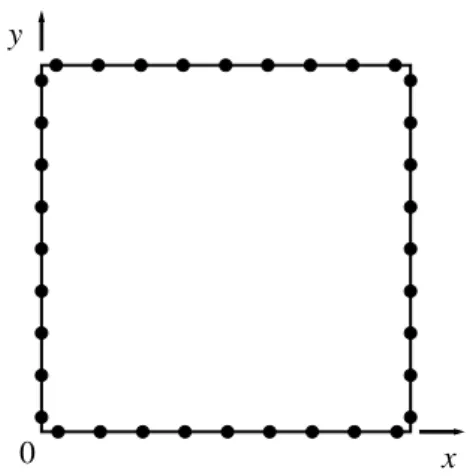
Uniformly distributed collocation points are chosen for the calculation (see Figure 2.3). The Taylor series for this problem are developed at point
0, 0 . Figure 2.4 is the influence of the number of collocation points for degree N=10, 20 and 30. It can be seen that the results may fluctuate and are not accurate enough if the collocation points are too few. The results become stable if the number of collocation points M is large enough. The degrees of freedom for Eq.(2.25) are 2N+1, thus M should be more than 2N+1 because collocation points should be more than the dimension of the vectorα in least-square method.
Figure 2.5 shows that the results get accurate with the increase of the degree. The maximal error becomes stable when the degree is more than 85. After that the accuracy stands under 14
24
Figure 2.4 The influence of the number of collocation points for Eq.(2.25), N=10, 20, 30
Figure 2.5 The influence of the degree N for Eq.(2.25),M 4N
2.5 Application of TMM to Kirchhoff plate problems
The Kirchhoff-Love theory of plates is a two-dimensional model for thin plates with small deflections. It was developed by extending Euler-Bernoulli beam theory in 1888 [71]. This theory makes the following assumptions:
1) The linear strain perpendicular to the middle plane can be disregarded; 2) The middle plane of the plate remains neutral during the deformation;
therefore the deformation from them can be disregarded.
The governing equation for a Kirchhoff-Love plate under transverse load is a fourth order partial differential equation that has no analytical solution except for a few plates of simple regular shapes. Thus numerical methods are used to approximately solve these problems. The formation of TMM for Kirchhoff plate will be introduced. Several cases are studied and results are discussed in the following part of this section.
2.5.1 Calculation of the shape functions
The governing differential equation for plates in the Kirchhoff plate theory is [72]:
4
0 , , ,
D w x y p x y x y (2.27)
wherew x y
,
is the lateral deflection,p x y
, is the lateral load, 3
2
0 12 1D Eh is the flexural rigidity of the plates,Eand are Young’s modulus and Poisson’s ratio respectively andhis the plate thickness.
If one can obtain a solutionw x y
,
, satisfying Eq.(2.27) and the given boundary conditions, bending moments, twisting moment and shear forces may be defined in terms of a functionwby: 2 2 2 2 2 2 2 2 2 2 2 3 3 3 2 3 3 3 2 1 , 2 2 x y xy x y x y w w M D x y w w M D y x w M D x y Q D w Q D w x y w w Q D x x y w w Q D y x y (2.28)
26
Eq.(2.27) and bending moments in Eq.(2.28) can be written in the form of second order derivatives: 2 2 2 2 2 2 2 0 0 xy y x M M M M p p x x y y x x (2.29)
2 2 11 12 16 2 12 22 26 2 16 26 66 2 x y xy w x M D D D w M M D D D D K y D D D M w x y (2.30)where [D] is the elastic matrix. Dij(i, j = 1, 2, 6) together are called flexural rigidity
which are determined by the material of the plates. For Kirchhoff plates with isotropic materials, the elastic matrix is:
0 1 0 1 0 0 0 1 D D (2.31)Now we have three equations with second order derivatives:
2 2 0 M p x x w k x x M D K (2.32)The unknowns
M and
K are split into two parts:
, , x y xy x y xy M M M M M M k k K k k k (2.33)the differential equation: one assumes that the dependence with respect toyis known and one considers the equation as a differential equation in x. The last equation in Eq.(2.32) can be represented withM andk:
11 12 13 11 12 13 12 22 23 12 13 23 33 13 . x y xy x x x y y x xy xy D k D k D k M D D D k M M D D D k D k D k M M D D D k D (2.34)
With the technique in Chapter 2.2, Eq.(2.32), Eq.(2.33) and Eq.(2.34) can be expanded with complete polynomials of order N. It can be concluded at the that equations at rank(m, n) are:
2 2 ( , ) 2 1 2, x x w k k m n m m w m n x (2.35)
2 2 2 2 1 , 2 , 1 1 1, 1 w n n w m n y k k m n m n w m n w x y (2.36) 12 12 13 13 . ( , ) ( , ) . ( , ) x x D D M k D k M m n k m n D k m n D D (2.37)
2 2 2 2 2 2 0 2 1 2, 2 1 1 1, 1 2 1 , 2 , xy y x x xy y M M M p x x y y m m M m n m n M m n n n M m n p m n (2.38)Eq.(2.35) - Eq.(2.38) give the recurrence formulae for the elements of TMM, as is shown in Table 2.1.
28
Table 2.1 Organization of the computation
Equation Derivation 2 2 x w k x (1) ( 1) ( 2, ) 1 ) , ( k m n m m n m w x y x w y w k 2 2 2 (2) ) 1 , 1 ( ) 1 )( 1 ( ) 2 , ( ) 1 )( 2 ( ) , ( n m w n m n m w n n n m k k D k D D M x . 13 12 (3) ( , ) ( , ) . ( , ) 13 12 n m k D n m k D D n m M x p y M y x M x Mx xy y 2 2 2 2 2 2 (4) ) 2 , 2 ( ) 1 )( 2 ( ) 1 , 1 ( ) 1 )( 1 ( 2 ) , 2 ( ) 1 ( 1 ) , ( n m M n n n m M n m n m p m m n m M y xy x
x y xy
x M D k D k D k 12 13 11 1 (5) ( , ) 1
( , ) 12 ( , ) 13 ( , )
11 n m k D n m k D n m M D n m kx x y xyWith the initial dataw
0,n w, 1,n k, x 0,n k, x 1,n , the approximate solution can be obtained as 4 3 0 N j j j w
P , where
0, 0 1, 1 1 2 0, 2 1 2 1 3 1 1, 3 3 4 3 j x x w j j N w j N N j N k j N N j N k j N N j N To calculate the thi shape functionPi,j
0 j 4N3
are chosen to be equal to 1 successively. The algorithm to choose is encoded as jfori 0 to4N 3 for j 0 to 4N 3 do if ji then