Numerical modelling of lateral viscosity variations in the Earth's mantle

NUMERICAL MODELLING OF

LATERAL VISCOSITY VARIATIONS

IN THE EARTH' S MANTLE

THESIS SUBMITTED AS A PARTIAL REQUIREMENT

FOR THE DEGREE OF MASTER OF SCIENCE

IN EARTH SCIENCES

BY

MARIE NICOLE THOMAS

UNIVERSITÉ DU QUÉBEC À MONTRÉAL Service des bibliothèques

Avertissement

La diffusion de ce mémoire se fait dans le respect des droits de son auteur, qui a signé le formulaire Autorisation de reproduire et de diffuser un travail de recherche de cycles supérieurs (SDU-522 - Rév.01-2006). Cette autorisation stipule que «conformément à l'article 11 du Règlement no 8 des études de cycles supérieurs, [l'auteur] concède à l'Université du Québec à Montréal une licence non exclusive d'utilisation et de publication de la totalité ou d'une partie importante de [son] travail de recherche pour des fins pédagogiques et non commerciales. Plus précisément, [l'auteur] autorise l'Université du Québec à Montréal à reproduire, diffuser, prêter, distribuer ou vendre des copies de [son] travail de recherche à des fins non commerciales sur quelque support que ce soit, y compris l'Internet. Cette licence et cette autorisation n'entraînent pas une renonciation de [la] part (de l'auteur] à [ses] droits moraux ni à [ses] droits de propriété intellectuelle. Sauf entente contraire, (l'auteur] conserve la liberté de diffuser et de commercialiser ou non ce travail dont [il] possède un exemplaire.»

LA MODÉLISATION NUMÉRIQUE

DES VARIATIONS LATÉRALES DE VISCOSITÉ

DANS LE MANTEAU TERRESTRE

MÉMOIRE PRÉSENTÉ

COMME EXIGENCE PARTIELLE

DE LA MAÎTRISE EN SCIENCES DE LA TERRE

PAR

MARIE NICOLE THOMAS

ACKNOWLEDGEMENTS

This work would not have been possible without the teachings, patience, and funding of my superviser Alessandro Forte; nor without continuai assistance and advice from Petar Glisovié, my windowless laboratory companion. l'rn also very grateful to Fiona Darbyshire for her excellent lectures, kind words, and generous support; and to Olivia Jensen, whose gracious assistance helped me to avoid the "leaky pipeline" of female physicists.

Many others have helped me complete this work; in particular, Utkarsh Ayachit pro-vided valuable support through the ParaView mailing list, and Jacqueline Austermann kindly shared her script for visualising dynamic topography output from ASPECT.

Computations for this thesis were made on the supercomputer Briarée from the Uni-versité de Montréal, managed by Calcul Québec and Compute Canada and funded by the Canada Foundation for Innovation (CFI), the ministère de l'Économie, de la sc i-ence et de l'innovation du Québec (MES!) and the Fonds de recherche du Québec -Nature et technologies (FRQ-NT). Additional simulations were run on the HiPerGator 2.0 supercomputer at the University of Florida.

LIST OF TABLES LIST OF FIGURES LIST OF ABBREVIATIONS 0 RÉSUMÉ 0 0 ABSTRACT 0 INTRODUCTION CHAPTER I

AN OVERVIEW OF MANTLE DYNAMICS 101 Historica1 background 0

102 Mantle rheology 0 0 0 0

10201 Geophysical evidence for short-term elastic behaviour 1.202 Geophysical evidence for long-term viscous behaviour 10203 Microphysical explanation

103 Mathematical background 10301 Governing equations

10302 Simplifications to constitutive equations 1.4 Presentation of the study 0 0 0 0 0 0 0 0 . 0 0 0 CHAPTER II

LATERAL VARIATIONS IN MANTLE VISCOSITY: A LITERATURE REVIEW 0 201 Introduction 202 Significance 203 Treatment 0 2.4 Conclusion VI VIl IX x Xl 3 3 5 6 7 10 Il 12 14 15 17 17 18

20

CHAPTER III

COMPUTATIONAL GEODYNAMICS 3.1 Overview . . . . . . 3.2 The finite difference method 3.3 The finite element method 3.4 ASPECT . . . .

3.5

3.4.1 Numerical framework 3.4.2 Models and parameters 3.4.3 Extensibility

3.4.4 Parallelism

3.4.5 Adaptive mesh refinement Conclusion

CHAPTER IV

MODELLING WITH ASPECT 4.1 Introduction . . .

4.2 Numerical mode!

4.2.1 Choice of tomography mode! . 4.2.2 Boundary conditions . . . . .

4.2.3 Calculation of dynamic surface topography 4.2.4 Updated viscosity profile .

4.3 Results and discussion . . 4.3.1 Parallel performance 4.3.2 Instantaneous mantle flow 4.3.3 Dynamic surface topography . 4.3.4 Importance of mesh resolution 4.3.5 Choice of tomography mode! . 4.4 Conclusion . . . . . . . . IV 24 24 25 25

26

28

58

CONCLUSION .. . BIBLIOGRAPHY . .

64

66

LIST OF TABLES

Table Page

4.1 Parameters used in the custom mode!, with values adapted mainly from Glisovié et al. (2012). . . . . . . . . . . . . . . . . . . . . . . . . . . . 41 4.2 Specifications for the HPG2 compute nodes used in the parallel

Figure

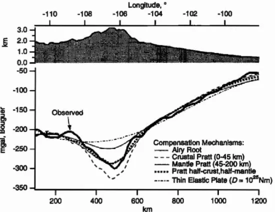
1.1 An illustration of isostatic compensation from Sheehan et al. (1 995). The top section represents the positive topography of the Rocky Moun-tains, and the thick black line below represents the negative observed gravity anomaly. The various dotted lines represent the predicted

grav-Page

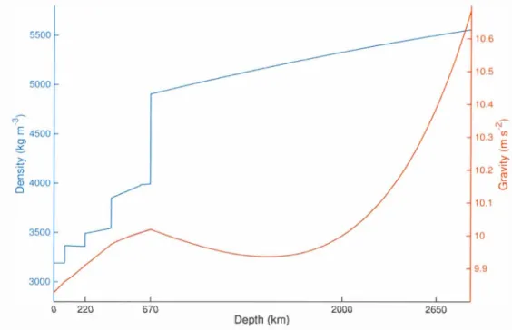
ity anomal y for different models of isostatic compensation. . . . . . . 9 4.1 The depth-varying profiles of density and acceleration due to gravity

used in the custom madel, adapted from PREM (Dziewonski and An-derson, 1981). . . . . . . . . . . . . . . . . . . . . . . . . . . . . . 37 4.2 The depth-varying thermal conductivity k, from Glisovié et al. (2012).

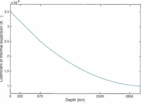
Four values of k were assigned to depths of 0 km, 80 km, 2650 km, and 2888 km and then linearly interpolated. . . . . . . . . . . . . . . . . . 38 4.3 The depth-varying coefficient of thermal expansion a, from Glisovié

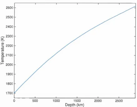
et al. (2012). The surface value of 3.5 x 10-5 _K-1 _{decreases Iinearly} to 2.5 x 10-5 _K-1 _{at a depth of 670 km. From there, a decreases in a} density-dependent manner to 1 x 10-5 _K-1 _{at the CMB. . . 39} 4.4 The depth-varying 'V2' viscosity profile (Forte et al., 201 0). 40 4.5 Adiabatic temperature profile with TsU!·f

=

=

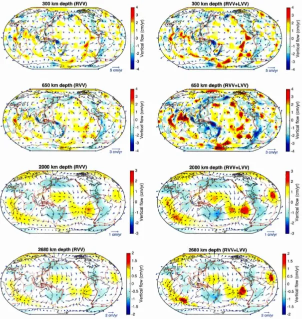
version of the custom model with 1.67 x 106 degrees of freedom was run on 16, 32, 64, 128, 256, and 512 cores. The black line indicates the total runtime, while the coloured lines indicate the runtime for each specifie simulation step. . . . . . . . . . . . . . . . . . . . . . . . . . . 49 4.7 Predicted mantle flow with (right) and without (left) modest LVV and

with a free-slip surface boundary condition. . . . . . . . . . . . . . . . 51 4.8 Calculated surface divergence without and with LVV, and calculated

V Ill

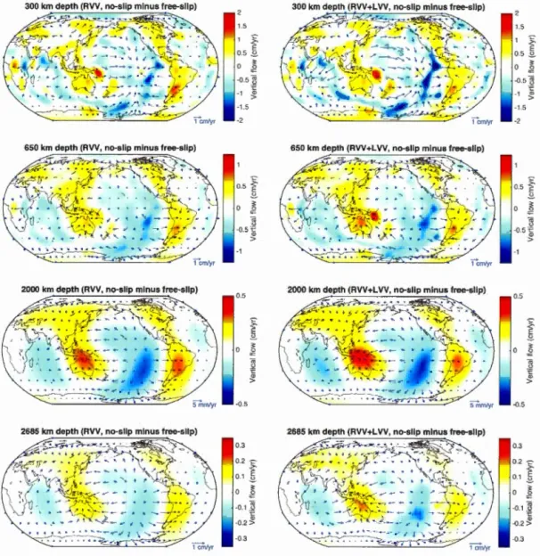
4.9 The impact of a no-slip surface condition on predicted mantle flow with (right) and without (left) modest LVV. . . . . . . . . . . . . . . . . . . 53 4.10 The dynamic surface topography produced accordi ng to Equation 4.4

and using a purely radial viscosity madel. . . . . . . . . . . . . . . . . 55 4.1 I The changes in dynamic surface topography produced when modest

LVV

(/3

=

a purely radial viscosity madel. . . . . . . . . . . . . . . . . . . . . . 59 4.13 Theimpactofsettingtheparameterinit ial global refinement

to 5 compared to 3. This figure shows the differentia] flow field at 300 km depth with free-slip boundary conditions and without lateral viscos-ity variations. . . . . . . . . . . . . .. .

4.14 The impact ofsetting the parameter Init ial global re finement 60

to 5 compared to 3. This figure shows the differentiai dynamic surface topography with free-slip boundary conditions and without lateral vis-cosity variations. . . . . . . . . . . . . . . . . . . . . . . . . . 61 4.15 The 3D mesh with the parameter Ini t ial global refinement

set to 5 (left) compared to 3 (right). . . . . . . . . . . . . . . . . . . . 62 4.16 Predicted mantle flow at 300 km depth using the GyPSuM (bottom)

and S40RTS (top) seismic tomography models. S40RTS produces an apparent upwelling about 30 degrees west of the EPR. . . . . . . . . 63

AMR adaptive mesh refinement

ASPECT Advanced Solver for Problems in Earth's ConvecTion

CitComS California Institute of Technology Convection in the Mantle -Spherical CMB core-mantle boundary DOF EPR FEM GIA GPS HPG2 LVV PREM RVV WPB VTU degrees of freedom East Pacifie Rise finite element method glacial isostatic adjustment Global Positioning System HiPerGator 2.0

lateral viscosity variations

Preliminary Reference Earth Mode! radial viscosity variations

weak plate boundaries

RÉSUMÉ

Cette étude modélise l'écoulement instantané du manteau terrestre en utilisant le code source ouvert ASPECT. Elle examine surtout l'impact des variations latérales de vis-cosité sur l'écoulement mantellique et sur la topographie dynamique de la surface. On utilise le profil de viscosité 'V2' de Mitrovica et Forte (2004), qui ne varie qu'en fonction de la profondeur. La composante latérale de la viscosité est calculée en sup-posant qu'elle dépend de la température selon une loi de type Arrhenius. Les variations de température viennent du modèle de tomographie sismique GyPSuM, qui intègre des données géodynamiques et des résultats d'expériences en physique des minéraux (Sim-mons et al., 2010). Les comparaisons entre des résultats obtenus par GyPSuM et par S40RTS, autre modèle de tomographie sismique de Ritsema et al. (2011), confirment que des vitesses des ondes de cisaillement ne suffisent pas pour résoudre la structure complexe du manteau terrestre.

De façon général, on trouve que les variations latérales de viscosité augmentent la vigueur de 1 'écoulement du manteau et atténuent la topographie dynamique de la sur-face. On cherche à varier l'amplitude des variations latérales de viscosité, mais la réso-lution numérique de ASPECT a du mal à converger même pour les variations modeste. On abordera des solutions et des orientations possibles pour des travaux futurs.

Mots clés: convection mantellique, rhéologie du manteau, viscosité, topographie dy-namique, tomographie sismique

The open-source code ASPECT is used to model the impact of lateral viscosity varia-tions on instantaneous mantle flow and dynamic topography.

The initial viscosity follows the geodynamically inferred 'V2' profile of Mitrovica and Forte (2004) which varies with depth alone. The lateral component of the viscosity is computed assuming an Arrhenius-type temperature dependence, with the perturbed temperature field given by the seismic tomography mode! GyPSuM, which unique! y in-corporates data from geodynamic observations and mjneral physics experiments (Sim-mons et al., 2010). Comparisons between GyPSuM and the S40RTS seismic tomo gra-phy mode! of Ritsema et al. (20 Il) confirms earlier findings that shear-wave velocities alone are not sufficient to characterise the complex, three-dimensional heterogeneities of the Earth's mantle.

In general, lateral viscosity variations are found to increase the vigour of mantle flow and to moderate the amplitude of dynamic topography. Different amplitudes are also investigated, but the ASPECT numerical sol ver demonstrates convergence problems be-yond modest lateral viscosity contrasts. Possible solutions and directions for future work are discussed.

Keywords: mantle convection, mantle rheology, viscosity, dynmruc topography, seis -mic tomography

INTRODUCTION

Viscosity is a key parameter in the study of thermal convection in the Earth 's mantle. The present study seeks to investigate mantle viscosity using the tools of computa-tional geodynamics, and specifically will examine the significance of lateral variations of viscosity in global simulations of mantle convection. The first chapter will develop a theoretical foundation to guide the chapters that follow, underlining the complex rhe-ology of the mantle and introducing the mathematical equations that govern thermal convection.

To provide more specifie context for this work, the second chapter will review past literature on the subject of lateral viscosity variations (LVV). We can infer from seis-mic data, convection-related observables, and mineral physics experiments that mantle rheology varies significantly not only with depth, but also laterally (e.g., Forte et al., 201 0). Large LVV spanning three or more orders of magnitude are necessary to account for stiff cratons and weak plate boundary zones in the lithosphere (e.g., Ghosh et al., 201 0). Mantle flow models that incorporate LVV can also predict sei smic anisotropy (e.g., Becker et al., 2008). It can be numerically challenging to implement LVV in the whole mantle, but comprehensive models should incorporate LVV on principle, as re-alistic mantle flow cannat be generated in their absence (e.g., Rogozhina, 2008; Forte et al., 2015).

The third chapter will present an overview of computational geodynamics, focusing mainly on the finite element method employed by ASPECT, or Advanced Solver for Problems in Earth's ConvecTion (Kronbichler et al., 2012), the open-source mantle convection code used for this study. The methods and results of the numerical madel

will be presented in the fourth chapter, with an emphasis on how mantle flow and dynamic surface topography change when LVV are taken into account. Finally, the conclusion will review important highlights from this work and propose directions for future research.

CHAPTER 1

AN OVERVIEW OF MANTLE DYNAMICS

1.1 Historical background

The puzzle-piece match between West Africa and the east coast of South America pro-pelled a few intrepid scientists towards the theory of continental drift in the earl y 20th century. Chief among them were Frank Bursley Taylor and Alfred Wegener, the latter of whom published an entire book on the subject in 1915. However, Wegener's ideas were widely panned by the scientific community. Critically, he had failed to provide a plausible mechanism that could drive these proposed surface movements (Schubert et al., 2004). Continental drift remained a fringe theory until it was revived by a grow-ing body of evidence, including the discovery of a rift on the Mid-Atlantic Ridge by Marie Tharp in the 1950s (Barton, 2002).

Tharp's collaborator Bruce Heezen inferred that the Mid-Atlantic Ridge was an ex-tensional structure and concluded that the Earth must be gaining volume over time (Davies, 2000). Dietz (1961) and Hess (1962) generally accepted the first premise but rejected the notion of an expanding Earth. Both proposed independently that new crustal material is formed at spreading ocean ridges, and that deep ocean trenches are areas of crustal convergence where the Earth 's surface a rea may be !ost, a process la ter identified as subduction. Direct evidence of seafloor spreading was identified by Vine and Matthews (1963) and Morley and Laroche! le ( 1964), who correctly interpreted the

magnetic stripes observed running pm·allel to ocean ridges as reversais in the polarity of the Earth's magnetic field over time. Emergent oceanic crust acquires thermoremanent magnetisation as it cools in the presence of the Earth's magnetic field and can preserve a record of the magnetic field direction while moving away from the spreading ridge over time. Continental drift, seaftoor spreading, and subduction were combined into a unified model of global plate tectonics by the late 1960s, with significant co ntribu-tions from Tuzo Wilson (Schubert et al., 2004). However, plate tectonics is a ldnematic mode) and cannot account for the driving force that was missing from Wegener's de -scription of continental drift.

Dietz and Hess had both proposed large-scale thermal convection cells in the mantle as providing the motive force behind seaftoor spreading. Tozer (1965) argued that mantle convection is inevitable due to the strong temperature dependence of silicate rheology, and Turcotte and Oxburgh (1967) related plate tectonics and mantle convection through a simple convection mode] in which the lithosphere was conceived as an upper thermal boundary layer that could travel along the top of a convection cell before descend -ing. Mantle convection has since been recognised as the driving mechanism behind the Earth's horizontal surface motions: cold material subducts and sinks, while hot mat e-rial rises from the mantle to form fresh crust on the ocean ftoor. In Wegener's time, the mantle was still considered too rigid to permit thermal convection, but shortly after the Mid-Atlantic Ridge was discovered, spreading of the ocean ftoor was also confirmed. The continental puzzle pieces had indeed been driven apart.

Though impossible to observe directly, the dynamic mantle expresses itself clearly through surface processes and other measurable phenomena, such as the geoid- an equipotential surface that undulates according to gravity perturbations across the globe, revealing information about the heterogeneous structure and composition of the solid Earth below. Glacial isostatic adjustment, or the ongoing relaxation of surface bulges and depressions formed under the weight of massive ice sheets during the Last Glacial

5

Maximum, provides further evidence of a non-rigid mantle.

The mantle is not a rigid body, but neither can it be described as having a true elastic response to applied stresses. Instead, the deformation of mantle rocks can be charac-terised as mainly elastic or viscous depending on the time scale of the applied stress: a property termed viscoelasticity. The following sections will explore this dual nature more thoroughly and present the physical and rheological laws that govern the long-term dynamics of the Earth 's mantle.

1.2 Mantle rheology

Rheology describes the flow and deformation of a viscous material. The mantle is vis-coelastic, responding in an elastic or viscous manner depending on the time scale of an applied stress. For deformations occurring on short to intermediate ti me scales, anelas-tic (nearly elasanelas-tic) processes dominate. This applies to seismic waves, free oscillations of the Earth, body tides, and the Chandler wobble. On time scales in excess of a few hundred years, the solid Earth exhibits fluid behaviour, giving rise to mantle convection and related geodynamic processes.

Viscoelastic materials are sometimes described as Maxwelljluids, and the characteristic time that separates anelastic deformation and viscous creep behaviour is referred to as the Maxwell tùne, given by the following:

( 1.1) where Tf is the long-term viscosity and I-L is the elastic modulus of rigidity. Average val-ues for the Earth's mantle are Tf = 1021 Pa · s and I-L = 100 GPa, which together give Trn ;::::::; 300 years. The transition time range is poorly understood, but ample geophysical evidence exists to support the short-term anelastic and long-term viscous comportment of mantle rocks (Forte, 2014).

1.2.1 Geophysical evidence for short-term elastic behaviour

Seismic waves provide a clear illustration of the solid Earth as an anelastic body. Body

waves propagate through the mantle with only a small amount of energy loss,

indi-cating travel through an imperfect elastic medium rather than a ftuid. In particular,

shear waves would not be able to propagate through the mantle at ali if it did not have

sufficient shear strength. Small energy attenuations, in which seismic waves Jose

vi-brational energy as heat, nonetheless reveal something of the viscous character of the

Earth (Karato, 2003). This energy dissipation may be characterised by a "transient"

viscosity (Anderson and Minster, 1979). Body waves have very short periods, typically

ranging from milliseconds to about a minute.

Earthquakes can also trigger the whole planet to vibrate like a struck bell, exciting the

free oscilllations of the Earth. Just as a vibrating string can be described in terms of its

characteristic normal modes, the displacement of the solid Earth can be represented as

the sum of one or more natural modes of vibration. Spheroidal modes describe radial

displacements inwards or outwards, while torsional modes represent displacements

par-alle! to the surface. Different free-oscillation modes of the Earth have been measured

with periods as short as just a few minutes and up to nearly one hour (Benioff et al.,

1961 ). These measurements con·espond to elasto-gravitational deformation that would not be physically possible if the sol id Earth behaved like a fluid on this time scale.

On a slightly longer time scale, the solid Earth experiences body tides under the grav i-tatiana! influence of the Sun and Moon. This deformation would not occur if the Earth

were completely rigid, and it would be much more pronounced if the solid Earth were

fluid. Body tides are also an elasto-gravitational deformation. Although numerous

7

12 hours; and diurnal, with periods of approximately 24 hours (Melchior, 1966).

The Chandler wobble, a free nutation of the Earth, provides further support of the mantle's anelastic behaviour on an intermediate time scale. The Chandler wobble is a principal component of polar wander and results from an uneven distribution of mass th at displaces Earth 's instantaneous rotational axis (Lowrie, 2007). The calculated pe-riod of this nutation is only about 305 days for an unyielding rigid-body Earth, while the observed Chandler wobble has T rv 435 days. However, taking anelastic deform a-tion into consideration together with surface oceans and a fluid outer core, calculated values are brought into close agreement with the observed period (Anderson and Min-ster, 1979).

1.2.2 Geophysical evidence for long-term viscous behaviour

When stresses are applied over geological time scales, the mantle appears to behave in a purely viscous manner. Sorne examples are continental drift driven by mantle convec-tion, and postglacial rebound in formerly glaciated regions. Other supporting evidence includes crustal isostasy and the agreement between the hydrostatic ellipticity of a ro-tating liquid and the flattening of the rotating Earth. This behaviour is characterised by a long-term or "steady-state" viscosity.

On millennial time scales, we can observe glacial isostatic adjustment (GIA): ongo-ing uplift and subsidence of the Earth 's surface in response to the retreat and even tuai disappearance of massive ice sheets since the end of the Last Glacial Maximum. Both the Laurentide and Fennoscandian ice sheets totally melted between 6,000 and 8,000 years ago and are a rich source of GIA data. In 1935, Norman Haskell was the first to estimate average mantle viscosity based on his analysis of Fennoscandian uplift. His estimate of about 1021 _{Pa · s has endured, even being reproduced through joint}

inver-sions of Laurentide uplift data and other geophysical constraints (Mitrovica and Forte,

2004). This behaviour should not be confused with elastic deformation, which is

com-pletely recoverable. Here, when the glacial Joad is removed, buoyancy forces return the surface to equilibrium, but any deformation incurred by steady-state creep is permanent

and can never be "reversed" in the thermodynamic sense (Van der Wal, 2009).

Thermal convection in the Earth's mantle occurs on even longer time scales, ranging

from millions to hundreds of millions of years, and gives ri se to the horizontal displace -ment of the Earth 's tectonic plates and the associated phenomenon of continental drift. These surface motions have traditionally been inferred from paleomagnetic data, but GPS satellites can now provide direct measurements of plate velocities as weil. Es ti-mates of surface plate velocities from geologie and geodetic data sets are remarkably similar (Forte, 2014).

Gravity measurements have led to a few different results which further suggest a vis-cous mantle. By the 17th century, pendulums were being used to measure gravity anomalies across the world, leading scientists to believe that the Earth was not a perfect sphere, but an ellipsoid. Isaac Newton postulated in his Principia Mathematica that the Earth was an oblate spheroid, or ftattened rather than football-shaped. One of his devotees, Alexis-Claude Clairaut, partook in an expedition to Lapland and developed his now-famous theorem to prove Newton's the01·y. Clairaut determined that, for a ro-tating ftuid at equilibrium, the hydrostatic ftattening is proportional to the square of the diurnal rotation rate. The present-day ellipticity of the Earth is remarkably similar to Clairaut's predictions for a rotating ftuid, providing further evidence of the mantle's long-term fluid character (Forte, 2014).

The concept of crustal buoyancy, or isostasy, arose from studies of the low grav ita-tional signais associated with high topography. ln 1855, John Henry Pratt conducted

plumb-9 Longitude, o -110 -108 -106 -~04 -102 -100 3.0 E 2.0 .li:. 1.0 0.0 -50 -100

....

a,

~

i

'

,

,

200 400 600 800 1000 1200

km

Figure 1 .1: An illustration of isostatic compensation from Sheehan et al. ( 1995). The top section represents the positive topography of the Rocky Mountains, and the thick black line below represents the negative observed gravity anomaly. The various dotted li nes represent the predicted gravity anomaly for different models of isostatic comp en-sation.

bob deviated far Jess from vertical than expected, given estimates of the excess mass represented by the mountains (Lowrie, 2007). Continental crustal rocks are Jess dense than mantle rocks, but a mountain range sitting flat on a solid mantle would nonetheless create a positive gravity anomaly relative to lower-lying regions. However, low grav i-tatiana) signais suggest that continents ftoat on the mantle like an iceberg at sea, with deep roots displacing the SUITounding mantle material. This displacement of denser material results in an overall deficit of mass and corresponding low-gravity anomal y, as

shown in Figure 1.1. For a more nuanced discussion of isostasy, the reader is referred to Lowrie (2007).

Gravity anomalies associated with density heterogeneities in the deep mantle can s imi-larly indicate long-term flow. For example, seismically fast regions below Pacifie sub-duction zones produce negative gravity anomalies at the surface, despite being asso-ciated with accumulations of cold slabs. Slabs are compositionally similar to mantle rocks but are denser by virtue of being colder, permitting them to subduct (McKenzie et al., 1974). Intuitively, the presence of positive density anomalies should produce positive gravity anomalies; however, in a convecting mantle, descending slabs are op-posed by flow-induced dynamic topography which can result in overall negative gravity anomalies (Forte et al., 20 15).

1.2.3 Microphysical explanation

The previous examples clearly illustrate the mantle's ability to flow over geological time periods. Mineral physics provides an explanation for this long-term viscous be-haviour: mantle rocks naturally contain atomic-scale defects in their crystalline struc-ture, allowing dynamic processes like creep to occur under conditions of constant stress and elevated temperature. When these conditions are maintained for a sufficiently long time, the mantle achieves steady-state flow characterised by an effective viscosity f1 (Forte, 2014):

( 1.2) where A is a dimensional constant, d is the effective grain size of mantle minerais, T

=

Il

Diffusion creep occurs at relatively low stress levels, small grain size, or both. This

type of deformation results in diffusive mass transport between grain boundaries of

mantle rocks, and the strain rate increases linearly with stress and depends significantly on grain size (Karato and Wu, 1993). ln terms of Equation 1.2, the effective viscosity

does not depend on stress (n

=

Dislocation creep occurs under conditions of high stress, large grain size, or both, and

is also referred to as power-law creep due to the nonlinear relationship between stress

and strain rate (Karato and Wu, 1993). Here, the effective viscosity depends on stress (n '"" 3) but not grain size (m

=

in the shallow upper mantle.

Olivine and other mantle minerais have been studied extensively in laboratory defor

-mation experiments in order to determine the rheology of the Earth 's mantle. However,

these results must be extrapolated to the irreproducible conditions of the mantle, where creep occurs on much longer time scales and at much Jower stresses. The validity of

such extrapolations is not clear (Karato, 2010). Olivine flow Jaws (e.g., Korenaga and Karato, 2008) are nevertheless used in many geodynamic models.

1.3 Mathematical background

The mantle can receive the same mathematical treatment as a fluid, owing to its Iiq-uid comportment over geological time. Different problems may cali for different ap

-proaches, but the mantle as a whole is typically treated as a viscous Newtonian fluid in numerical simulations of thermal convection.

1.3.1 Governing equations

The fundamental equations of ftuid dynamics are derived from the princip les of conser -vation of mass, energy, and momentum (Landau and Lifshitz, 1987). The problem of mantle convection additionally requires an equation of state relating the density tote m-perature and pressure and a rheological description relating the stress and strain rate. The latter has already been described by Equation 1.2 in terms of the mantle's effective viscosity.

Considering an infinitesimal volume, conservation of mass implies that the rate of change of mass in the volume must be equal and opposite to the mass lost through flow:

o

p

-

+

V

.

0

at

where p is the density and u is the flow velocity.

( 1.3)

Next, conservation of energy implies that the rate of change of energy must be equal to the rate of heat production Jess the rates of heat Joss through convection and conduction. This gives the temperature equation:

aT dp

PCp7fi

=

+

Q

Finally, conservation of momentum implies that the rate of change of momentum must be equal to ali forces acting on a given volume of the ftuid mantle, namely surface forces (arising from viscous stresses) and body forces (due to gravity):

du

p -

=

v

+

13

where a is the stress tensor and g is the gravity vector. This equation is simply

New-ton's second law of motion.

The total stress tensor a is:

a = -Pl +T ( 1.6)

where P is the total pressure, I is the identity matrix, and T is the viscous or deviatoric

stress tensor, which represents the non-hydrostatic component of stress. It is written in

Einstein notation as:

T

=

=

+

~d

i

j

U

k

,

k)

+

where 77 is the effective viscosity, 5i.i is the identity tensor (i.e., 5ij

=

=

.J

,

=

#

.J),

Equation 1.6 can be used to rewrite the stress divergence term in the conservation of

momentum (Equation 1.5):

du

p - =

(

-

V'

+

V'

·

T

)

+

dt

Conservation of mass and momentum can together describe the flow field, given an

equation of state p(P, T):

(1.9)

where T1

=

compressibility of the mantle material, and P1

=

perturbations. The term p0 is a reference density given by the hydrostatic reference

state of the mantle, where u

=

V'

where Po and p₀ are the reference hydrostatic pressure and density, respectively.

motion:

du

p -

V

(cSP)

+

v

.

+

(cSp)

g

dt

where

cSP

cSp

( 1.12)

The last term will be ignored as compressibility does not make first-order contributions.

1.3.2 Simplifications to constitutive equations

A number of simplications can be made to the governing equations of Section 1.3.1.

First of ali, mantle convection occurs on a ti me scale many times longer than that of the

local acoustic velocity. Thus, sound waves can be ruled out as possible solutions to the flow equations through the anelastic liquid approxùnation:

V ·

(pu

)

=

in which the term ~j has been ignored in the conservation of mass equation (Forte et al.,

20 15). Furthermore, it is assumed th at the density perturbations p1 ( r,

e

,

first-order contributions to the equations of conservation of mass and energy and can

therefore be neglected.

Similarly, the ti me derivative of velocity ~~ in the conservation of momentum equation

may be neglected due to the very high viscosity of mantle rocks. This is the infinite Prandtl number approxùnation, a limit at which fluid motion occurs slowly enough to neglect inertial effects.

The second viscosity coefficient À in the viscous stress tensor Tij describes the energy dissipation associated with volume changes. Density changes arising from mantle flow

15

thermal equilibrium, and the second viscosity coefficient À in Equation 1.7 can

there-fore be ignored (Landau and Lifshitz, 1987), rendering the viscous stress tensor entirely

deviatoric:

2

T_'· · _·.7

=

(

u

·

+

'1 1,.7 J,1 3 tJ o;, (1.14)

Furthermore, many numerical models assume a linear Newtonian rheology for the

whole mantle, meaning that the viscosity rJ depends on temperature and pressure (or

depth) but not stress or strain rate. This approach simplifies the solving process but

fails to accurately represent areas where nonlinear rheology may be present, such as

subduction zones and other high-stress regions.

1.4 Presentation of the study

The dynamic nature of the Earth's mantle can be observed indirectly through its many

expressions on the surface, such as tectonic plate motions and glacial isostatic

adjust-ment. Mantle convection is governed by rheological laws and the partial differentiai

equations outlined in Section 1.3.1. The third chapter will discuss the numerical

meth-ods used to solve these equations, with a heavy emphasis on ASPECT, a relatively new

open-source code designed to solve thermal convection and similar mathematical

prob-lems.

This study will use ASPECT to investigate the impact of lateral viscosity variations on

numerical simulations of mantle convection, and particularly their impact on

calcula-tions of dynamic topography. Together with the non-hydrostatic geoid, dynamic

sur-face topography is one of the most important convection-related observables. Without

mantle convection, the surface topography of the Earth would be entirely due to lateral

variations in crustal thickness and density; in other words, to isostatic compensation of

the isostatically compensated crustal signal from the total observed surface topography of the Earth. It is important to note that the accuracy of the resulting estimates depends entirely on the uncertainties present in the crustal mode!, which may be considerable.

CHAPTER II

LATERAL VARIATIONS IN MANTLE VISCOSITY: A LITERATURE REVIEW

2.1 Introduction

In 1687, Isaac Newton introduced the term defectus lubricitatis to describe the internai resistance of a fluid, which he proposed was "proportional to the velocity with which the parts of the fluid are separated from one another" (Newton, 1729). This describes, in the parlance of modern fluid dynamics, the linear stress-strain relation of a Newtonian fluid. At the time, Newton was mainly concerned with disproving the physics of his predecessor, René Descartes, and specifically the vortex theory of planetary motions through a ftuid ether. One century later, the hydraulic engineer Pierre du Buat studied the temperature dependence of viscosity, but the concept was not full y formalised until 1822, when Claude-Louis Navier introduced coefficients of viscosity into the equations offtuid motion (Jacobson, 1991).

Viscosity is a key parameter in the study of mantle convection, and inversions of geo-physical data have indicated that the mantle's effective viscosity varies significantly with depth. The simplest numerical models assume an isoviscous mantle, but more r e-alistic estimates of viscosity can be determined and employed using modern computa-tional methods. Two-layer viscosity profiles allow for a rheological distinction between the upper and lower mantle, with a viscosity increase typically occurring near 670 km

depth. This coïncides with a seismic discontinuity and major phase change from spinel

to silicate perovskite, and while the viscosity increase could be due to a change in grain

size, this increase has also been detected as deep as 1200 km (Schubert et al., 2004).

Changes around this depth could be related to a progressive "dewatering" of perovskite

(Rudolph et al., 2015), the deformation behaviour of ferropericlase (Marquardt and

Mi y agi, 20 15), or a different phenomenon entirely. These diverse possibilities speak to

the extreme complexity of mantle rheology.

More elaborate viscosity profiles have been determined through joint inversions of data

from post-glacial rebound, mineral physics experiments, and convection-related

ob-servables (Mitrovica and Forte, 2004; Steinberger and Calderwood, 2006). Generally,

radial viscosity profiles are constrained in the top rv 1000 km of the mantle by Haskell 's

value of 1021 _{Pa · s, a robust early estimate of average mantle viscosity based on}

Fennoscandian post-glacial uplift (Haskell, 1935). Lateral viscosity variations (LVV)

have only recently received serious consideration, and different studies have reached contradictory conclusions as to their signi ficance and rel evan ce in numerical models.

The present chapter will present an overview of literature concerning lateral viscosity

variations in the Earth's mantle.

2.2 Significance

The effective viscosity of the mantle has only rarely been accorded three-dimensional

treatment, often reduced to simple depth layers or even a single value. Lateral

vis-cosity variations are sometimes considered an unnecessary addition to global models

of mantle convection, not !east because their inclusion can dramatically increase s

im-ulation runtime and resource usage. There is also conflicting research as to whether

convection-related observables can be adequately described in terms of a radial vis -cosity profile alone. Furthermore, constraints on mantle viscosity can be quite poor.

19

For instance, laboratory experiments on rock deformation are limited, requiring sig

-nificant extrapolations to mantle conditions and generating large uncertainties in the process (Karato, 201 0). Olivine, the most abundant and best-studied mineral of the upper mantle, remains so poorly constrained in terms of activation energy, activation volume, grain size, and water content asto allow for the vastly different constructions of upper-mantle viscosity, from essentially constant to linearly increasing in the shallow asthenosphere (King, 2016). From this perspective, LVV certainly do seem to make models unnecessarily complicated.

On a local scale, laterally homogeneous viscosity is often an unrealistic assumption,

particularly around subduction zones. LVV have also increasingly been investigated in the context of glacial isostatic adjustment. Seismic tomography has indicated signifi-cant heterogeneities in the mantle beneath East and West Antarctica, which Kaufmann et al. (2005) proposed as a large temperature-viscosity difference due to a deep cratonic root un der East Antarctica. Van der Wal et al. (20 15) fou nd that a 3D viscosity provides better fits to GPS uplift data and significantly affects the spatial pattern of uplift rate, and that low vi cosities (

<

very sensitive to recent changes in ice thickness.

Rogozhina (2008) has argued that, regardless of their apparent impact on the geoid and other observables, lateral viscosity variations are a necessary component of compreh en-sive mantle flow models. lt has been shown that only lateral viscosity variations can excite mantle flow in such a way as to generate the toroïdal component of surface plate motions (Forte et al., 2015). Spherically symmetric models fail to produce a toroïdal component similar in energy to the poloidal component of flow.

2.3 Treatment

Earl y studies involving LVV were carried out al most exclusively in 20 Cartesian geom-etry, and most numerical models have neglected them entirely. The reader is referred to Moucha et al. (2007) and Rogozhina (2008) for an overview of these early inves ti-gations.

Relatively few studies have explored LVV in the who le mantle. Kaban et al. (20 14a) looked at the combined effect of whole-mantle LVV and weak plate boundaries (WPB). They found that both were necessary to explain certain features of the geoid and dy -namic surface topography, but that the effect of WPB was more dominant by far. They cautioned that considering the effects of whole-mantle LVV or WPB separately could lead to enoneous results.

On the other hand, Moucha et al. (2007) found little effect from LVV on dynamic topography and the geoid, especially compared to uncertainties in published seismic tomography models. Austermann et al. (20 15) fou nd an impact on dynamic topography due to LVV, but only in terms of change over time. Neither of these studies considered WPB, although the latter employed a rigid (no-slip) surface boundary condition, which is locally valid for Antarctica.

Most studies have modelled LVV assuming that an Arrhenius-type temperature depen-dence is dominant. Ghosh et al. (20 1 0) investigated LVV using two methods: assigning specifie viscosity contrasts to tectonic regions, and calculating a temperature depen-dence given by:

TJ = TJa · exp (E · 6.T) (2.1)

where TJa is the reference viscosity, E is a parameter controlling the strength of the temperature dependence, and 6.T

=

- - - -- - - -- - - -- - - -- - - -- - - -- - - -- -- -- - - -- - - ,

21

unchanged, but that the magnitude was affected by as much as 20%.

Petrunin et al. (2013) modelled LVV up to ...,5 orders of magnitude and found a strong

effect on mantle dynamics and the geoid. The authors obtained lateral temperature

anomalies by applying a constant velocity-density scaling factor to the S40RTS seismic

tomography mode! of Ritsema et al. (2011), and from there modelled strong LVV using

a homologous temperature approach:

( T,n(T) )

'T!(T

,

e

,

cj;

)

=

Ao(T)

T

a

(T)

+

6T(T

,

e

,

cj;

)

where the melting temperature T,n was calculated using two different depth-dependent

functions for the upper and lower mantle,

T

a i

m-perature variations

6T

thermal expansion coefficient,

E

Ao(T)

the radial viscosity constant.

Ranalli (2001) modelled LYV in the whole mantle using lateral temperature variations

from the sei smic tomography model of Su et al. ( 1994 ), assuming the following relation

between temperature anomalies 6.T and shear wave velocity v:

(2.3)

where the coefficient of thermal expansion a had a depth-varying distribution. Ass

um-ing a regime dominated by diffusion creep and constant strain rate or constant viscous

dissipation power-law creep, rather than by constant stress power-law creep, LVV were

found to vary from one to four orders of magnitude, being more pronounced in the

uppermost and lowermost mantle.

Glisovié et al. (20 15) modelled grain size variability and fou nd that lateral variations

in grain size attenuate LVY. This work resulted in a new picture of LVV dist

ribu-tion through the whole mantle, while also revealing that traditional assumptions about

the upper mantle below 200 km could be modelled in terms of diffusion creep only, they

used the experimentally determined flow law for dry olivine (Korenaga and Karato, 2008):

d'"'

1JcL

=

E,~~v,)

where d is the grain size, m1 is a grain-size sensitivity exponent, A1 is a scaling con-stant, E1 and Vj are the activation energy and volume of dry olivine, p is the pressure,

R

T

in terms of vacancy diffusion for MgSi0₃ perovskite:

kd2T

1Jct=

-AXvVDpv (2.5)

where k is Boltzmann's constant, A is a geometrical factor for modelling grain

bound-ary sliding, Xv is the vacancy concentration, V is the molecular volume of perovskite,

and Dpv is the effective diffusivity in perovskite that is controlled by Mg diffusion.

Glisovié et al. (2015) varied the values of activation enthalpy for grain growth

H

gr

and for diffusion

H.

Hg

,)

H

::;

and local regions of reduced viscosity in the middle lower mantle associated with hot

upwellings. However, results from the

Hg

,·/

H

=

relationship between temperature and viscosity due to the strong effect of grain size.

This mode! suggests that hot upwellings in the lower mantle could actually be stiffer

than average due to larger grain sizes. Therefore, the traditional assumption of an

Arrhenius-type temperature dependence for vacancy diffusion in the lower mantle may

not be entirely valid.

The rheological impact of grain size and other microphysical parameters has also been

investigated on a local scale. Barnhoorn et al. (20 1 1) used both diffusion and

disloca-tion flow laws for olivine to mode! the upper mantle beneath Scandinavia and found

LVV up to 3-4 orders of magnitude, mainly due to large temperature anomalies present

dif-23

fusion creep were identified as active deformation mechanisms in the upper mantle

beneath Scandinavia on the time scale of glacial isostatic adjustment, and their relative

contributions were found to be sensitive to microstructural parameters like grain size,

water content, and stress levels present during deformation.

2.4 Conclusion

The dynamic impact of lateral viscosity variations remains poorly understood.

How-ever, it has been shown that spherically symmetric models are unable to produce a com-prehensive picture of global mantle flow. In particular, LVV are necessary to excite the toroïdal component of mantle flow (Forte et al., 2015). To avoid inconect results, care must be taken to investigate possible interactions between LVV and other conditions

such as weak plate margins (Kaban et al., 2014a).

The spatial distribution of LVV also remains unclear, though strong lateral hetero-geneities are implied in the upper mantle, particularly in the lithosphere. Mantle rhe-ology depends strongly on temperature, pressure, strain rate, and grain size; but many

studies have calculated LVV assuming a simple Arrhenius temperature dependence.

This could be a drastically inval id assumption for the lower mantle in particular (Giisovié et al., 20 15). Ranalli (200 1) has asserted th at rheology of the transition zone and lower mantle will remain highly speculative until more is known about average grain sizes and the pressure dependence of creep in gamet and perovskite.

Direct modelling of LVV has been extremely limited until very recently. Continuing

advances in high-performance computing and high-pressure mineral physics will en-able ever more sophisticated numerical models and move us towards the development of a more complete description of mantle rheology.

COMPUTATIONAL GEODYNAMICS

3.1 Overview

Though partial differentiai equations can sometimes be solved without numerical meth-ods, those that govern mantle convection generally require them. The field of compu-tational geodynamics began to emerge around 1970, with the earliest one-dimensional models giving way to a flurry of two-dimensional investigations of subduction, thermal convection, and other tapies (Gerya, 2010). The first three-dimensional mantle convec-tion models appeared in the mid-to-Iate 1980s, and the field has since seen remarkable advances by virtue of increasing computing power.

Various numerical techniques have been developed to solve partial differentiai equa-tions, including finite difference, finite element, finite volume, and spectral methods (Schubert et al., 2004). The equations described in Section 1.3.1 apply to a con-tinuum, or an infinite number of points, and thus present an infinite number of un-known variables. Quasi-analytical solutions can be obtained through the spectral and pseudo-spectral methods, but most numerical techniques obtain an approximate solu-tion through discretisation of the original equations, which reduces them to a discrete problem with a fini te number of unknowns (Johnson, 2009).

25

will focus on the open-source code ASPECT, beginning with a brief overview of the

finite difference and finite element methods, then explaining the inner workings of

As-PECT while addressing its strengths as weil as its shortcomings.

3.2 The finite difference method

The fini te difference method ob tains a discrete problem by replacing derivatives in the

original equations with differences computed between two discrete points. For instance,

ô

A

ô

6A

6 x (3.1)

where 6A = A2 - A1 is the difference in function A between two points, which on the x-axis are separated by a distance 6x

=

im-plies an infinitesimal difference, shortening the distance between points .-r 1 and x2 will

increase the accuracy of the finite difference approximation (Gerya, 2010). The same

approach can also approximate higher-order derivatives. In this way, partial differentiai

equations are reduced to sets of linear equations of finite differences. These differences are calculated on a numerical mesh, which approximates the continuum with a finite

number of points. The finite difference method typically uses a regular grid and solves

the problem only at each nodal point; the method is thus ill-suited for problems

involv-ing complex geometry or boundary conditions, which motivated the development of other techniques.

3.3 The finite element method

The finite difference method attempts to solve the derivatives directly. By contrast, the

finite element method (FEM) attempts to solve the integral form of a differentiai

equa-tion instead. The integral version is also known as the "weak formulation" because

equation, which is sometimes too rigorous to be solved. FEM discretises the domain into smaller pieces as weil, but solves the problem over each such "finite element" to

obtain a quasi-continuous solution. Accuracy and numerical stability can be major is

-sues with FEM, but it can also handle complex geometries and material discontinuities

far better than the fini te difference method. This technique forms the backbone of

man-tle convection code like CitComS (Zhong et al., 2000) and ASPECT.

3.4 ASPECT

ASPECT, short for Advanced Solver for Problems in Earth 's ConvecTion, is an

open-source code that employs finite elements to solve the equations governing thermal

con-vection (Kronbichler et al., 2012). The project mainly focuses on mantle dynamics of

the Earth, but the code has a modular structure to accommodate a wide range of

re-search interests. Simulations are controlled with input files in which parameters can

be specified to dictate everything from the rheology and geometry of a model to the

desired output variables. Users can modify the default parameters of existing models

or implement extensions of the source code to suit their needs. Compositional fields

are another key feature which enables the study and tracking of heterogeneities in the

mantle.

ASPECT builds upon the sound infrastructure of the deal. II fini te elements library, which in turn depends on TRI LINOS for parallellinear algebra and p4est for parallel mesh handling. These projects are actively maintained and serve much broader

com-munities than ASPECT alone, providing a sol id foundation and allowing developers and

27

3.4.1 Numerical framework

The deal . II finite elements library forms the backbone of ASPECT, providing

func-tionality for adaptive meshes, pm·allel computing, and linear algebra solvers for the

systems of equations that describe thermal convection. ASPECT requires that the li

-brary be compiled with p4est for distributed adaptive mesh support (Burstedde et al.,

20 Il) and TRI LINOS for parallel Iinear algebra support (Heroux et al., 2005).

ASPECT solves the same fundamental equations described in Section 1.3.1, but as a

finite element code, it approximates the solutions using linear basis functions. For the

Stokes system comprising the equations of mass and momentum conservation, these

basis functions cannot be arbitrarily chosen due to the Ladyzhenskaya-Babuska-Brezzi (LBB) condition, which requires that the problem be well-posed. ASPECT fulfils this

stability condition using a Taylor-Hood scheme in which the polynomial degree of the

pressure basis functions is one less than that used for the velocity elements (Kronbichler

et al., 2012). By default, ASPECT employs quadratic elements for the velocity and

linear elements for the pressure. This is far more computationally expensive than the

lowest-element scheme, in which the pressures are piecewise constant and the velocities

are piecewise linear, but using higher-order elements improves the numerical stability

of the solver as weil as the accuracy of the solution. ASPECT similarly uses quadratic

elements for the temperature, but this polynomial degree can theoretically be reduced

to save on computation time in studies where the temperature field is of little interest

and does not affect the accuracy of the velocity and pressure fields.

Once the Stokes and temperature equations are fully discrete, each can take the form

of a system of equations to be conditioned into a more tractable form and then solved

through an iterative method. Iterative solvers work through a problem repeatedly, at

each step using the previous solution as a new starting point until the final a

These systems are not always linear, however. For example, Heister et aL. (2017) have acknowledged compressibility as one of the most challenging issues in the

develop-ment of ASPECT, since the mass conservation equation is only linear for incompress

-ible models. The compressible case contains extra terms which introduce nonlinearity

that must be linearised and solved iteratively in order to obtain a solvable linear system.

Choosing the appropriate solving schemes and preconditioners can be difficult, and

ev-ery choice involves a certain amount of tracte-off. This process is described in detail

and quantified using benchmarks in Heister et aL. (2017).

3.4.2 Models and parameters

The community has developed numerous models and benchmarks for users to explore

and build upon, ali of which are described in the manual (Bangerth et aL., 2016). Simple

models, like thermal convection in a two-dimensional box, are a computationally

inex-pensive way to familiarise oneself with the code orto investigate specifie features. For

instance, the Sinker wi th averag ing benchmark uses a circular density contrast

within a two-dimensional box to demonstrate how material properties can be averaged to avoid sharp discontinuities which would place too much strain on the numerical sol ver.

Most parameters have a default value, so input files for simple models can be very short.

Since the code works in two spatial dimensions by default, the following line would be

29

1 set Dimension 3

The material model, which describes material parameters of the mantle such as viscos

-ity and density, can be set with just a few li nes:

subsection Material madel

set Madel name = simple compressible

end

Without further specification, ASPECT will use default values for viscosity and any other available parameters. To illustrate a less generic input, the following lines could

be included to specify a spherical geometry from the core-mantle boundary (reM 8

=

3481 km) to the surface (rs'U1'f

=

=

4000 K and TsU1·f

= 4

subsection Geometry madel

set Madel name = spherical shell

subsection Spherical shell

set Inner radius 3481000

set Outer radius

=

end end

subsection Boundary temperature madel

set Madel name = spherical constant

subsection Spherical constant

set Inner temperature 4000

set Outer temperature = 400 end

end

Along with the graphical solution and other requested outputs, ASPECT generates a file

specified-even if they were not used in the simulation-and extensive commentary

for each line. This allows results to be easily reproduced and removes any confusion about which parameters produced a given solution.

3.4.3 Extensibility

The so-called cookbooks provided in the manual are an excellent starting point for new users, but most projects require a high degree of custom input and extensions to the source code. Fortunately, ASPECT was designed to be extensible, making it trivial to include custom code for the material description, initial conditions, geometry, graphi-cal outputs, and so on. Custom files can be included without affecting the functionality of the original source code-although that, too, could be modified by advanced users

wishing to alter the fundamental way in which ASPECT solves the basic equations.

3.4.4 Parallelism

ASPECT supports parallel computing, meaning that its work can be split into different tasks across multiple processing units. For instance, graphical solutions are generated

by default as Visualization Toolkit Unstructured (VTU) files, a format that allows

dif-ferent processors to calculate the solution on different sections of the working mesh. These partial solutions can be easily collected into the full geometry, for instance by

visualisation software like Para View, without the need to communicate to a single

pro-cessor which would write a single output.

Computing clusters are typically comprised of many nodes, machines which have soc

k-ets containing multiple cores, also known as processors or CPUs. Different computing

tasks require different approaches to resource management. Sorne jobs require ac

31

increase performance-each task would still be stuck waiting for the same resource.

Only spreading the job across cores on different nodes would remove this bottleneck.

However, other jobs would be slowed down by such a configuration, since

communica-tion ti me between nodes can introduce significant dela ys (Hager and Gerhard, 20 Il).

Ideally, any code would run twice as fast after doubling the number of cores used, but

real code requires that some work be done seri ally, and there is al ways a li mit where

per-fOI·mance no longer increases. Parallel code projects typically provide speedup charts to

help users choose the most economical resource allocation for their jobs. These charts

illustrate the relation between performance and cores used. No such resource exists in

the ASPECT manual, likely due to the high degree of variability between simulations,

but Heien et al. (20 12) provide parallel performance data for a simple spherical shell

model.

The efficiency of parallel code also depends on an even distribution of work among cores. Wh en Joad balancing, AsPECT currently considers only the degrees of freedom

(DOF), a number determined by the dimensions and refinement of the mesh, as weil

as the discretisation of the original equations. Performance is not optimised for tracer

particles and other computationally expensive elements of the code, although it is po

s-sible to choose a strategy that adaptively retines the mesh according to tracer particle

density, viscosity variability, or another relevant criterion. Nonetheless, one mode! with

one million DOF could run for thirty minutes on 12 processors, white another with the

same DOF could take hours on many more processors due to a more complex mantle

3.4.5 Adaptive mesh refinement

Numerical simulations can be calculated on an even mesh, but accurate solutions for mantle convection require a very fine resolution, which can be computationally expen -sive. ASPECT allows for adaptive mesh refinement (AMR), a process by which the

numerical mesh can be locally refined and coarsened over time, or simply within the

first time step. Typically, the user will want to refine areas of interest on the mesh, which may contain higher relative errors due to strong heterogeneities in the velocity field or other calculated parameters. The mesh can also be coarsened for regions where the solution is more homogeneous and has smaller relative errors. This uneven retine -ment can remain constant after the first time step, or it can be allowed to adapt over

time as the solution evolves-following a subducting slab, for example.

ASPECT solves a probJem on an initial mesh with uniform cell spacing defined by the

Initial global re finement parameter. When the Initial adaptive refinement

parameter is non-zero, the code then uses one or more refinement strategies to compute

an error field and flags sorne fraction of cells for refinement or coarsening. For exam

-ple, setting the parameter Re finement fraction to 0. 5 will flag 50% of ali cells

for refinement, choosing those with the highest relative en·or. ASPECT currently imple -ments strategies that can flag for different compositions; specified boundaries; spatial

variabilities of the density, viscosity, or temperature; among others.

An adaptively refined mesh can achieve the same overall accuracy as a regular mesh that has been uniformly refined to the same highest resolution (Kronbichler et al., 201 2).

Moreover, this method can be up to a thousand times faster. AMR thus represents one of the major strengths of ASPECT.