DOCTORAT DE L'UNIVERSITÉ DE TOULOUSE
Délivré par :
Institut National Polytechnique de Toulouse (INP Toulouse)
Discipline ou spécialité :
Energétique et Transferts
Présentée et soutenue par :
Mme CHIARA GALATI
le mercredi 13 décembre 2017
Titre :
Unité de recherche :
Ecole doctorale :
Etude numérique et expérimentale de la distribution de fluide dans un
échangeur de chaleur compact à plaques
Mécanique, Energétique, Génie civil, Procédés (MEGeP)
Laboratoire de Génie Chimique (L.G.C.)
Directeur(s) de Thèse :
M. LAURENT PRAT M. CHRISTOPHE GOURDON
Rapporteurs :
M. HASSAN PEERHOSSAINI, UNIVERSITE PARIS 7 M. LAURENT FALK, CNRS
Membre(s) du jury :
M. HASSAN PEERHOSSAINI, UNIVERSITE PARIS 7, Président M. CHRISTOPHE GOURDON, INP TOULOUSE, Membre
M. LAURENT PRAT, INP TOULOUSE, Membre M. LIONEL CACHON, CEA CADARACHE, Membre Mme MARIA ADELA PUSCAS, CEA SACLAY, Membre
...e a Te,
che mi hai sempre protetto sotto il
Ce travail de thèse s’inscrit dans le cadre du programme R&D du CEA en support au système de conversion d’énergie à gaz du prototype industriel de Réacteur à Neutrons Rapides refroidi au Sodium (RNR-Na). Cette technologie représente une alternative aux cycles Rankine conventionnels à eau/vapeur, ayant pour avantage principal l’élimination du scenario accidentel de réaction sodium-eau. Cependant, la faible capacité de transfert de chaleur du gaz nécessite une technologie d’échangeurs compacts à plaques avec un nombre élevé de canaux à alimenter. Coté sodium, une section minimale de passage est nécessaire pour éviter le risque de bouchage par impureté. Cela induit de très faibles pertes de pression dans le faisceau qui, couplées à une condition de vitesse élevée à l’entrée, génèrent un risque réel de mauvaise distribution du débit. Les performances d’échange thermique et la tenue mécanique du composant sont alors dégradées.
L’objectif principal de ce travail de thèse a été de résoudre ce problème de mauvaise distribution, en s’appuyant sur une conception innovante (BREVET FR16 57543), sur une stratégie de calcul numérique et l’établissement d’une base de données expérimentale pour la validation des travaux théoriques.
Le nouveau système de distribution sodium se compose d’un collecteur d'entrée dont le design permet de guider la trajectoire du jet et d’un système de bifurcation de canaux qui augmente les pertes de pression dans le faisceau. De plus, des communications latérales entre les canaux sodium aident à homogénéiser davantage le flux.
Deux installations expérimentales ont été conçues pour caractériser l'écoulement dans les canaux de bifurcation et dans le collecteur d'entrée. La conception des maquettes a permis de quantifier leur effet sur la distribution du flux entre les canaux. La base de données aérodynamiques PIV acquises a permis de valider les modèles numériques et de prouver l’efficacité du système de distribution proposé.
Après avoir validé les modèles de turbulence CFD et la stratégie d'étude de la distribution dans le module SGHE, une optimisation de chaque composant du système de distribution de sodium a été réalisée.
Le travail de cette thèse s’achève par la description de la conception optimale retenue pour la phase actuelle du projet ASTRID.
Mots Clés : Echangeur compact à plaques, Mauvaise distribution, Mécanique des fluides
numérique (CFD), Vélocimétrie par image des particules (PIV), Jet tridimensionnel, Jets parallèles.
This PhD work was motivated by the CEA R&D program to provide solid technological basis for the use of Brayton power conversion system in Sodium-cooled Fast nuclear Reactors (SFRs). Multi-channel compact heat exchangers are necessary for the present application because of the low heat transfer capacity of the gas foreseen. In ASTRID project, a minimum size of Na channels section is required to avoid the plugging risk. However, this induces very low pressure losses in the bundle. Considering an additional inlet flow condition, a real risk of bad flow distribution remains. As a result, the thermal performance and thermal loading of the heat exchanger degrades due to it.
The main goal of this work was to overcome the flow maldistribution problem by means of an innovative design of sodium distribution system (PATENT FR1657543), the development of a numerical strategy and the construction of an experimental database to validate all theoretical studies.
The innovative sodium distribution system consists on an inlet header which tries to guide the evolution of the impinging jet flow while a system of bifurcating pre-distribution channels increases pressure drops in the bundle. Lateral communications between pre-distribution channels are introduced to further homogenize the flow.
Two experimental facilities have been conceived to study the flow behavior in bifurcating channels and in the inlet header, respectively. At the same time, their effect on the flow distribution between channels is evaluated. The acquired PIV aerodynamic database allows to validate the numerical models and to prove the design basis for the proposed distribution system.
Once having validated the CFD turbulence models and the strategy to study the flow maldistribution in the SGHE module, a decisive and trustworthy optimization of each component of the sodium distribution system has been performed.
Finally, an optimal configuration has been proposed for the actual phase of ASTRID project.
Keywords: Compact Heat Exchanger, Flow maldistribution, Computational Fluid
Dynamics (CFD), Particle Image Velocimetry (PIV), Three-dimensional jet flow, Parallel jets.
A l’issue de ce travail de recherche, je suis convaincue que la thèse n’est pas seulement une expérience professionnelle mais une expérience de vie. On se retrouve souvent seule face à des problèmes qu’on ne sait pas forcement résoudre et qui nous donnent le temps de découvrir nos faiblesses mais aussi nos points forts. Durant cette phase délicate, le soutien d'un grand nombre de personnes m’a été indispensable. Leur générosité, leur bonne humeur et leur intérêt manifesté à l'égard de ma thèse m'ont permis d’évoluer et de progresser.
En première lieu, je tiens à remercier Monsieur Lionel Cachon pour la confiance qu'il m'a accordée en me confiant une mission très intéressante. Je le remercie pour m’avoir accompagné pendant ces trois dernières années, pour m’avoir apporté son savoir-faire et son savoir-être et pour être tout simplement une image professionnelle par laquelle on apprend beaucoup.
Je souhaiterais exprimer ma gratitude à mon directeur de thèse, monsieur Laurent Prat, qui malgré la distance et son emploi du temps très chargé a toujours été présent dans les moments difficiles. Il m’a appris qu’on peut avoir de grandes responsabilités tout en restant disponible pour les autres. Je dois aussi le remercier pour toutes les conférences et les formations auxquelles j'ai pu participer, cela m'a donné la possibilité de présenter mes travaux à l'international et d'améliorer mes compétences sur des thématiques spécifiques. Merci à Christophe Gourdon pour avoir été l’encadrant le plus optimiste de ma thèse, merci pour sa participation scientifique ainsi que le temps qu’il a consacré à ma recherche Merci à Monsieur Sylvain Madelaine, pour m’avoir accueilli dans son laboratoire depuis mon stage de fin d’étude. J’ai été extrêmement sensible à ses qualités humaines d'écoute et de compréhension tout au long de ce travail doctoral.
Quand, en Février 2014, je suis arrivée au CEA depuis l’Italie, je n’étais qu’une jeune étudiante pas très douée en français et assez timide. Mais j'ai eu la chance de travailler dans un laboratoire avec des personnes uniques qui m’ont tout de suite fait sentir comme chez moi.
Merci à Corinne et Stéphane, chaque matin vous étiez présentes pour discuter et rire ensemble avant de commencer la journée de travail. Merci à Xavier et Christophe, les piliers de la salle de calcul, les discussions avec vous m’ont toujours permis d’approfondir mes compétences scientifiques et mon savoir-vivre.
électrique de mes plaques. Des giga octets de merci !
Je ne pourrais jamais assez remercier Thomas Marchiollo, qui restait tous les après-midis après 17h, pour écouter mes plaintes et pour me soutenir quand tout paraissait difficile. Tu ne m’as pas seulement aidé à concevoir des veines fluides et des maquettes mais mon projet de thèse dans sa globalité. Tu as partagé avec moi DANAH, nous y avons cru ensemble et nous avons réussi à la réaliser. Merci pour ton amitié.
Merci à Isabelle Tkatschenko et David Guenadou pour m’avoir accueilli dans leur laboratoire et pour m'avoir laissé tout le temps nécessaire pour pouvoir compléter de façon adéquate mes mesures. Valérie et Fabienne, merci pour votre patience et pour m’avoir dédié beaucoup de temps afin d’obtenir des résultats expérimentaux exploitables. Un grand merci à Jean Philippe et Philippe, les co-équipiers plus atypiques qui se sont toujours débrouillés pour réparer DANAH et qui m’ont appris avec leur style de vie à apprécier le travail et relativiser dans les moments difficiles.
Merci aussi à Giulio Mancini et Giovanni Baldi, qui se sont chargés de plusieurs parties importantes de ce travail et qui m’ont permis d’avancer dans des axes de recherche que je n’aurais jamais pu investiguer autrement.
Merci à Elena d'être ma binôme de bureau cool et pleine d’énergie qui m’a accompagné dans cette expérience. Merci pour ton amitié et pour les longues discussions sincères. Merci à tous mes amis italiens expatriés comme moi, merci pour tous les bons moments passés ensemble.
Un merci particulier à mon mentor, Francesco Vitillo. Même après la fin de sa mission de tuteur de stage, il était là pour me montrer les différentes étapes à franchir et me permettre d’avancer. Il m’a fait profiter de son expérience pour éviter des erreurs et je le remercie d’avoir cru en moi. Il est surement la personne qui a enrichi le plus ma connaissance scientifique.
Merci également à l’atelier et à toutes l’équipe du LGC qui ont su m’accueillir à Toulouse et me supporter pendant tous les problèmes de la maquette EASY-B. Sans leur
engagement il n’aurait pas été possible de mener à bien ces mesures.
Merci à Alain et Alec les gardiens de l’INP ENSIACET, qui ont mis à ma disposition l’école à des horaires improbables et qui m’ont tenu compagnie pendant les longs post-traitements de mesures.
familial. Merci à Mamma et Papà, pour avoir été toujours présents pendant les choix importants de ma vie. Merci pour votre patience et votre aide quotidienne. pour faire toujours tout le possible pour m'aider. Merci Roberta pour ton soutien et tes conseils précieux qui deviennent de plus en plus indispensables dans ma vie. Merci Francesco, pour être un frère si spécial qui fait mon bonheur et ma joie de vivre. Enfin merci à Nonno et Nonna pour votre affection infinie et pour être mon plus grand exemple de Famille. Merci à Titti et Stefania, les amies de toujours qui continuent à me supporter depuis 25 ans ! Et merci à tous mes amis du sud, qui m’ont permis de me ressourcer pendant mes vacances.
Enfin, le plus grand merci revient à Pierre-Yves, qui est entré dans ma vie seulement à la moitié parcours de thèse et il a accepté sans aucune hésitation de rester à mes côtés pour construire la plus belle histoire d’amour. Merci pour ta patience et ta bienveillance, mais également merci de m’avoir transmis ta sérénité et ta joie qui ont été nécessaires pour surmonter mes plus grandes difficultés.
Chapter 1 ... 24
Context and scope of the work ... 24
1.1. Context ... 24
1.2. The ASTRID Project ... 28
1.2.1. The compact Sodium Gas Heat Exchanger (SGHE) ... 30
1.3. Scope of the work ... 33
1.4. Thesis Outline ... 34
Chapter 2 ... 36
Bibliographic Study ... 36
Flow Maldistribution in Compact Heat Exchanger ... 37
2.1. Consecutive Manifold ... 38
2.1.1. Theoretical studies of flow manifold ... 39
2.1.2. Experimental studies of flow manifold ... 45
2.1.3. Computational studies of flow manifold ... 48
2.2. Normal -Header ... 51
2.2.1. Experimental studies of flow in Normal -Header ... 51
2.2.2. Computational studies of Normal-Header ... 57
2.3. Bifurcation Manifold ... 62
2.3.1. Experimental studies of bifurcation manifold ... 64
2.3.2. Computational studies of bifurcation manifold... 66
2.4. Adopted strategy ... 71
2.4.1. Flow maldistribution conditions in ASTRID Compact Heat Exchanger ... 71
2.4.2. ASTRID Compact Heat Exchanger requirements ... 73
2.4.3. Header solutions ... 75
Chapter 3 ... 85
Experimental Facilities ... 85
3.1. EASY-B: Experimental Analysis of SYmmetric Bifurcating channels ... 88
3.1.1. Experimental Mockups ... 89
3.1.2. PIV measurement system ... 92
3.1.3. Pressure measurement system ... 105
3.1.4. Mass flow measurement system ... 110
3.1.5. Mass flow data from pressure measurements ... 112
3.1.6. Conclusion ... 114
3.2. DANAH: Distribution Analysis of Na in Headers ... 115
3.2.1. Experimental Mockup ... 116
3.2.2. PIV equipment in DANAH experimental campaign ... 122
3.2.3. Experimental program definition ... 124
3.2.4. PIV measurements calibration and testing ... 127
3.2.5. Measurements statistical convergence ... 128
3.2.6. Experimental uncertainty evaluation ... 130
3.2.7. Flow Inlet Conditions ... 135
3.2.8. Flow Symmetry ... 136
3.2.9. PIV Measurements at the outlet header ... 138
3.2.10. Conclusion ... 150
Chapter 4 ... 151
Numerical Study of Flow Pattern in Pre-Distribution Channels ... 151
4.1. CFD Numerical approach for the SGHE flow analysis... 151
4.1.1.3. The Anisotropic Shear Stress Transport (ASST) Model ... 155
4.1.2. Computational model and flow boundary conditions ... 157
4.1.3. CFD solver setting ... 159
4.1.4. Grid sensitivity ... 159
4.1.5. The selection of the CFD numerical model ... 162
4.2. Model Validation and Flow Analysis ... 168
4.2.1. Longitudinal evolution of principal flow ... 168
4.2.2. Mass Flow Rate Validation ... 176
4.3. Parametric study and Design optimization of the header design ... 178
4.3.1. The bifurcation system in SGHE module – Optimization Criteria ... 178
4.3.2. The bifurcation system – Parametric Study ... 180
4.3.2.1. Influence of the bifurcation structure ... 182
4.3.2.2. Effect of inlet Reynolds number ... 184
4.3.2.3. Effect of channel length after the first bifurcation ... 186
4.3.3. Distribution performance comparison and conclusion ... 187
4.4. A new design for ASTRID SGHE bifurcating channels ... 190
4.5. Conclusions ... 192
Chapter 5 ... 194
Numerical Study of Flow Pattern in Compact Heat Exchanger ... 194
5.1. CFD Numerical approach for the SGHE flow analysis... 195
5.1.1. Turbulence numerical models ... 195
5.1.1.1. The Realizable k- ε model ... 196
5.1.1.2. The Linear Pressure Strain – Reynolds Stress Model ... 197
5.1.2. Computational model and flow boundary conditions ... 198
5.2. Model Validation and Flow Analysis ... 209
5.2.1. Inlet header Flow ... 209
5.2.2. Outlet header Flow ... 215
The validation of the flow maldistribution factor ... 217
5.3. Parametric study and Design optimization of the header design ... 221
5.3.1. Overview of the SGHE and optimization parameters ... 221
5.3.2. Influence of pressure drop ∆𝐏 ... 223
5.3.3. Influence of h... 224
5.3.4. Influence of l ... 227
5.3.5. Influence of h, l being constant ... 228
5.3.6. Influence of 𝛂 ... 229
5.3.7. Influence of adding connection: pre-bundle ... 232
5.3.8. Distribution performance comparison and proposed solution for ASTRID SGHE 233 5.4. Conclusions ... 235
Chapter 6 ... 237
Conclusions and Perspectives ... 237
6.1. Conclusions ... 237
6.2. Perspectives ... 239
6.2.1. Thermo-mechanical analysis of proposed SGHE design... 239
6.2.2. Optimization of communication zone in bifurcating channels ... 242
6.2.3. Experimental validation of channel communications ... 242
APPENDIX II ... 247
Optimization of channel connections – “Pre-Header” ... 247
II.1. Channel connections ... 249
II.2. Longitudinal connection height, h ... 250
II.3. Influence of longitudinal obstacles ... 253
II.4. Inlet mass flow maldistribution intensity ... 254
II.5. Mass flow inlet peak position ... 254
APPENDIX III ... 256
III.1. EASY-B: Mockup 1 ... 256
III.2. EASY-B: Mockup 2 ... 257
III.3. EASY-B: Mockup 3 ... 258
III.4. DANAH: Inlet header (1) ... 259
III.5. DANAH: Inlet header (2) ... 260
III.6. DANAH: Outlet header... 261
III.7. DANAH: Bundle channel wedge ... 263
Fig.1. 2 – Nuclear electricity production during last 50 years ... 24
Fig.1. 3 - Introduction of IV Generation Nuclear Power ... 25
Fig.1. 4 - French experience on SFR reactors ... 26
Fig.1. 5 - Pool-type Sodium-cooled Fast Reactor ... 27
Fig.1. 6 - Overall schedule of the ASTRID project ... 28
Fig.1. 7 - Gas Power Conversion System (PCS) Layout ... 29
Fig.1. 8 – Sodium Gas Heat Exchanger 2014’ design ... 31
Fig.1. 9 - SGHE Module ... 32
Fig.2. 1 – Compact heat exchanger – Inlet Header ... 37
Fig.2. 2 - Major types of manifolds ... 38
Fig.2. 3 - Manifold configurations: (a) U-flow or parallel flow configuration; (b) Z-flow or reverse-flow configuration. Pressure profile in (c) U-flow configuration, (d) Z-flow configuration ... 39
Fig.2. 4 – Geometrical parameters influencing flow distribution [20] ... 40
Fig.2. 5 - Schematic diagram of U-Type manifold [20] ... 40
Fig.2. 6 - Control volume for intake (a) and exhaust (b) header [20-21] ... 41
Fig.2. 7 –Effect of flow area ration M on flow distribution [19] ... 43
Fig.2. 8 - Effect of Ratio of header length to diameter E on flow distribution [19] ... 43
Fig.2. 9 - Effect of flow resistance in lateral channels ξ on flow distribution [19] ... 44
Fig.2. 10 - Trapezoidal header [23] ... 46
Fig.2. 11 - Multi-step header [23] ... 46
Fig.2. 12 - Inclined grid installed in the header [23] ... 46
Fig.2. 13 - Modified header with tube baffle [23] ... 46
Fig.2. 14– Flow maldistribution vs Volume flow rate for U-type flows with the tested headers ... 47
Fig.2. 15 - Comparison between experimental and numerical flow ratio 𝛽 for two different inlet mass flows Q ( 𝑡 = 3.5 𝑚𝑚 𝑎 𝑜𝑟 𝑡 = 18.5 𝑚𝑚 (𝑏)) ... 48
Fig.2. 16 - CFD velocity streamlines for consecutive manifold with t = 3.5mm (a) and t=18mm (b) ... 49
Fig.2. 17- Comparison of predicted and measured axial velocity profiles (a) and axial RMS velocity profiles in plane of symmetry (b). Inlet flow rate 3.3 x m3/s [25] ... 50
Fig.2. 18 - Typical Compact Heat Exchanger - Normal-Header [3] ... 51
Fig.2. 19 – Geometrical features of tested header [27] ... 52
Fig.2. 23 - Second Header B and C [28] ... 53
Fig.2. 24 - Distribution of the difference flow velocity at Re 1000 and Re 3000 [28] ... 54
Fig.2. 25 - Test header configuration and v [29] ... 55
Fig.2. 26 - PIV velocity vectors and streamlines of cross-section 1 (a) and 2 (b) [29] ... 55
Fig.2. 27 - Example of a perforated grid (Configuration F) [29] ... 56
Fig.2. 28 - Velocity distribution of different headers at Re 6x10⁴ [29] ... 56
Fig.2. 29 - PIV velocity vectors and streamlines of cross-section 1 (a) and 2 (b) after the installation of the perforated grid [29] ... 57
Fig.2. 30 - Comparison between experimental and numerical data of average velocity at Re 2100 [33] ... 58
Fig.2. 31 - Velocity vector and streamlines of cross section 1: (a) PIV [29] (b) CFD Wen [29] (c) CFD Raul [34] ... 59
Fig.2. 32 - Velocity vector and streamlines of cross section 2: (a) PIV [29] (b) CFD Wen [29] (c) CFD Raul [34] ... 59
Fig.2. 33 - Definition of the channels at the outlet of header [35] ... 60
Fig.2. 34 - Maldistribution parameters along with x direction at different Re [35] ... 60
Fig.2. 35 - Pressure drop versus different type of headers at Re 1x10⁵ [35] ... 60
Fig.2. 36 - Type B – Perforated grid with holes in-line arrangement [35] ... 61
Fig.2. 37 - Type C - Perforated grid with holes staggered arrangement [35] ... 61
Fig.2. 38 - Bifurcation and Consecutive Manifold [19] ... 62
Fig.2. 39 - Consecutive Manifold (a) - Normal-Header (b) - Bifurcation Manifold (c) [36] . 62 Fig.2. 40 - Different types of manifold with lateral channel communications [36] ... 63
Fig.2. 41 - Flow distributor constructed by T-shape bifurcation of channels (a) Tree-shaped structure (b) – Circular-shaped structure (c) [41] ... 64
Fig.2. 42 - A close-up view of the flow distributor and Pitot tube set-up [41] ... 65
Fig.2. 43 - Measured velocity profiles at the centerline of height of channel [41] ... 65
Fig.2. 44 - Experimental and numerical results of non-dimensional velocity distribution 67 Fig.2. 45 - Sharp fillet (SF) (a) and Curvature fillet (EF) (b) [43] ... 68
Fig.2. 46 - Velocity of the diffluent flows at a T joint (a1) Re 187, (b1) Re 810, (c1) at Re 1560 – Transverse vortices [45] ... 69
Fig.2. 47 - Streamlines of the diffluent flows at a T joint (a3) Re 187, (b3) Re 810, (c3) at Re 1560 – Longitudinal vortices [45] ... 69
Fig.2. 48 - Velocity of the diffluent flows at a T joint Re 810– Transverse vortices [45] ... 70
Fig.2. 52 - Modified U-type manifold ... 76
Fig.2. 53 - Velocity field in “pre-faisceau” zone ... 76
Fig.2. 54 - Velocity field in modified U-type manifold with inlet admission ... 77
Fig.2. 55 - Selected geometry of Normal-Header (II.1 function) ... 77
Fig.2. 56 - Na/N2 plates arrangement (I.1 function) ... 78
Fig.2. 57 - Velocity field in double grid Normal –Header with inlet admission ... 78
Fig.2. 58 - Sodium plate: Channel communications and Bifurcation system ... 80
Fig.2. 59 - Operating principle of channel connections in a 10x10 bundle channel ... 82
Fig.3. 1 - Overview of PLATEAU facility ... 86
Fig.3. 2 - Overview of EASY-B Pilot Installation ... 88
Fig.3. 3 - Experimental schematic circuit EASY-B ... 89
Fig.3. 4 - Mockup geometry: Test sections 1 (a), 2 (b) and 3 (c) ... 90
Fig.3. 5 - PMMA Test Section 2 ... 91
Fig.3. 6 - System components for PIV [51] ... 92
Fig.3. 7 - PIV Image evolution [51] ... 93
Fig.3. 8 - Nano L PIV Laser (left side) and its displacement system (right side) ... 94
Fig.3. 9 - Rhodamine B – Test section1 (left) and PS FluoRed – Teste Section 2 (right) exposed by the Nd-YAG light sheet ... 95
Fig.3. 10 - Imager Pro X Camera (left) and its displacement system (right) ... 96
Fig.3. 11 – PIV measurement plane in z-direction ... 97
Fig.3. 12 - PIV measurements fields in x-y direction ... 98
Fig.3. 13 - Camera calibration using channel boundaries ... 99
Fig.3. 14 – Camera Calibration using SlidOverTime LaVision Post Processing ... 99
Fig.3. 15 - 1R_Test Section 2 -Velocity field and monitoring points position ... 100
Fig.3. 16 - SONDE 2: u, v velocity (left) and u’, v’ Velocity Fluctuations (right) ... 101
Fig.3. 17 – Mockup displacement device ... 103
Fig.3. 18 – Velocity field at 18mm from the inlet admission – Test Section 2 ... 105
Fig.3. 19 - KELLER Pressure transmitters ... 106
Fig.3. 20 - Pressure transmitter position: Mockup 1, Mockup 2 and Mockup 3 ... 106
Fig.3. 21 - Working principle of a capacitive pressure transducer ... 107
Fig.3. 22 - Pressure measurement chain ... 108
Fig.3. 23 - EASY-B electronic weighing system ... 110
Fig.3. 24 - Sartorius Combics 1 CAW1P*L precision balances ... 111 Fig.3. 25 – Empirical correlation between pressure drop and mass flow – Test Section 2 . 113
Fig.3. 28 – Inlet Header (1) ... 117
Fig.3. 29 - Outlet Header ... 118
Fig.3. 30 – PIV target (left) and its displacement system (right) ... 119
Fig.3. 31 – DANAH bundle channel (left) and detail on a single plate (right) ... 119
Fig.3. 32 - Section of DANAH bundle channel ... 120
Fig.3. 33 - Pre-Header component (left) and Pre-Header in DANAH mockup (right) ... 120
Fig.3. 34 - DANAH Support - Structure A ... 121
Fig.3. 35 –DANAH Support – Structure B ... 121
Fig.3. 36 - Nano L PIV Laser (left side) and its displacement system (right side) ... 122
Fig.3. 37 - Laser alignment at the outlet header ... 122
Fig.3. 38 – Capture of seeding particles at the inlet header ... 123
Fig.3. 39 - Camera ... 124
Fig.3. 40 - Green DANAH experimental campaign and inlet header (1) ... 125
Fig.3. 41 - Blue DANAH experimental campaign and inlet header (2) ... 125
Fig.3. 42 - PIV measurement planes at the inlet (left) and outlet (right) header ... 126
Fig.3. 43 - Camera Calibration on PIV target at the inlet (left) and outlet (right) header .. 127
Fig.3. 44 - Camera calibration on mockup dimensions ... 128
Fig.3. 45 - PIV measurements statistical convergence at the inlet header ... 129
Fig.3. 46 - PIV measurements statistical convergence at the outlet header (BD_2_75) ... 130
Fig.3. 47 - PIV standard uncertainty at the inlet header (BD_2_75) ... 131
Fig.3. 48 - Scatter light and background noise at the inlet header (BD_2_75) ... 132
Fig.3. 49 - PIV standard uncertainty at the outlet header (BD_2_75_NC) ... 132
Fig.3. 50 – Raw Data- PIV Image zoom on the outlet header ... 133
Fig.3. 51 - PIV image before (right) and after (left) the INSIGHT 4G Pre-processing ... 133
Fig.3. 53 – PIV velocity profile on the admission pipe ... 136
Fig.3. 54 – Symmetric planes ... 136
Fig.3. 55 - PIV velocity field at I-Plane2 (left) and I-Plane 4 (right) ... 137
Fig.3. 56 - PIV velocity field at I-Plane1 (left) and I-Plane 5 (right) ... 137
Fig.3. 57 - PIV velocity profile at the outlet header (O-Plane 18) ... 138
Fig.3. 58 - Coanda Effect [64] ... 139
Fig.3. 59 - Schematics of a free turbulent jet ... 140
Fig.3. 60 - Schematics of two-parallel turbulent jets [67] ... 140
Fig.3. 61 - Typical flow pattern of plane jets [70] ... 141
Fig.3. 65 - Y velocity profile at different y positions downstream the channel outlet ... 145
Fig.3. 66 – Y Velocity peaks of at the outlet of the 32 channels of plate 20 ... 146
Fig.3. 67 - Schematic map of selected channels for flow analysis ... 147
Fig.3. 68 - 3D y velocity profile ... 148
Fig.3. 69 - Channel obstruction in DANAH bundle ... 148
Fig.3. 70 - PIV velocity field downstream the plugged channel ... 149
Fig.3. 71 - Y velocity profile downstream the plugged channel ... 149
Fig.3. 72 – PIV velocity field at O-Plane 25 (left) and 27 (right) nearby the obstructed channel ... 150
Fig.4. 1 - Computational Model ... 158
Fig.4. 2 - PIV and CFD inlet velocity profile ... 158
Fig.4. 3 - Coarse, Medium and Fine mesh of channel cross-section ... 160
Fig.4. 4 – Mesh detail of bifurcation zone ... 161
Fig.4. 5 - Wall Y+ contour of bifurcating channel ... 161
Fig.4. 6 - Mesh Independence Study - Velocity profile at line O ... 162
Fig.4. 7 - Selected lines for turbulence model comparison ... 163
Fig.4. 8 - Experimental vs numerical velocity profile at line O ... 163
Fig.4. 9 - Experimental vs numerical velocity profile at line C ... 164
Fig.4. 10 - Experimental vs numerical velocity profile at line G ... 164
Fig.4. 11 - Experimental vs numerical u’ Reynolds Stress at line C ... 165
Fig.4. 12 - Experimental vs numerical u’ Reynolds Stress at line G ... 165
Fig.4. 13 - Experimental vs numerical v’ Reynolds Stress at line C... 166
Fig.4. 14 - Experimental vs numerical v’ Reynolds Stress at line G ... 166
Fig.4. 15 - Velocity field comparison on the middle plane of Mockup 1 (PIV data at the left and k- ASST computation at the right) ... 169
Fig.4. 16 - Longitudinal evolution of flow in Mockup 1 - 𝑣 velocity profiles ... 170
Fig.4. 17 - CFD velocity Streamlines and vectors at the middle plane of Mockup 1 ... 172
Fig.4. 18 - Velocity vectors on plane normal to the mean flow direction at line B (left) an E (right) ... 173
Fig.4. 19 - Velocity field comparison on the middle plane of Mockup 2 (PIV data at the left and k-ω ASST computation at the right) ... 174
Fig.4. 20 - Velocity profile 𝑣 at line A on left (left) and right (right) generated branch... 174
Fig.4. 21 – Velocity profile 𝑣 at line B on left (left) and right (right) generated branch... 175
Fig.4. 25 - Computational domain and boundary conditions ... 181
Fig.4. 26 – Structures of flow channel bifurcation – R0 and R4 bifurcation ... 182
Fig.4. 27 - Velocity profiles at line 1 (continue curve) and line 2 (dashed curve)... 183
Fig.4. 28 - Velocity streamlines of flow at channel bifurcation - R0_25-25 and R4_25-25 183 Fig.4. 29 - Flow maldistribution 𝜎𝑏 for different Reynolds numbers ... 185
Fig.4. 30 - Pressure drops for different Reynolds numbers ... 185
Fig.4. 31 - Flow maldistribution 𝜎𝑏 for different length L1 and L2 ... 186
Fig.4. 32 - Pressure drops for different length L1 and L2 ... 187
Fig.4. 33- Two-level bifurcating channel parametric study ... 187
Fig.4. 34 - Two-level (left) and three-level (right) bifurcating channel ... 190
Fig.4. 35 - Velocity vectors at "zone 2" of Mockup 3 ... 191
Fig.4. 36 - Velocity field comparison on the middle plane of Mockup 3 (PIV data at the left and k-ω ASST computation at the right) ... 192
Fig.5. 1 - Computation Model ... 199
Fig.5. 2 – PIV and CFD inlet velocity profile ... 201
Fig.5. 3 - Mesh view ... 202
Fig.5. 4 –Coarse, Medium and Fine Mesh at the inlet header ... 202
Fig.5. 5 - Mesh detail at the outlet header ... 203
Fig.5. 6 - Mesh Independence Study - Velocity profile at line 1 ... 204
Fig.5. 7 - Wall Y+ contour at the inlet header ... 205
Fig.5. 8 - Selected lines for turbulence model comparison ... 206
Fig.5. 9 - Experimental vs numerical mean velocity profile at line 1 ... 206
Fig.5. 10 - Experimental vs numerical mean velocity profile at line 2 ... 207
Fig.5. 11 - Experimental vs numerical mean velocity profile at line 3 ... 207
Fig.5. 12 - Experimental vs numerical u'u' Reynolds Stress at line 2 ... 208
Fig.5. 13 - Experimental vs numerical v'v' Reynolds Stress at line 2... 208
Fig.5. 14 - Velocity fields on Plane 3 (PIV data on top and Realizable K-ε computation on the bottom) ... 210
Fig.5. 15 - Velocity fields on I-Plane 2 and I- Plane 4 I (PIV data on top and Realizable K-ε computation on the bottom) ... 211
Fig.5. 16 - Velocity fields on I-Plane 1 and I- Plane 5 I (PIV data on top and Realizable K-ε computation on the bottom) ... 212
Fig.5. 17 – Physical evolution of a confined jet flow ... 213
the bottom) ... 216
Fig.5. 21 - PIV and CFD velocity profiles at y=21mm on Plane 20 O ... 218
Fig.5. 22 -PIV Velocity profile distribution on the entire bundle ... 219
Fig.5. 23 - CFD Velocity profile distribution on the entire bundle ... 219
Fig.5. 24 - CFD and PIV Plate Maldistribution Factors ... 220
Fig.5. 25 - SGHE Layout (left) and optimization parameters at the inlet header (right) .... 222
Fig.5. 26 - Flow maldistribution factor for different pressure drop ∆P ... 224
Fig.5. 27 -3D Mass Flow Distribution and velocity contour for different inlet header heights (h= 0 mm and h= 75 mm) ... 225
Fig.5. 28 - 3D Mass Flow Distribution and velocity contour for different inlet header heights (h= 150 mm and h= 250 mm) ... 226
Fig.5. 29 - Flow maldistribution factor for different pressure drop ∆P ... 227
Fig.5. 30 - 3D Mass Flow Distribution and for different jet impingement position ... 228
Fig.5. 31 - 3D Mass Flow Distribution and for different header height h ... 229
Fig.5. 32 - 3D Mass Flow Distribution for different admission angles ... 230
Fig.5. 33 - Flow maldistribution factor for different admission angles 𝛼 ... 231
Fig.5. 34 - Velocity streamlines at the inlet header for 𝛼 = 0° ... 232
Fig.5. 35 -3D Mass Flow Distribution without and with channel communications ... 233
Fig.5. 36 – Flow distribution performance – Optimization study ... 234
Fig.6. 1 – Proposed design solution SGHE (2017) ... 238
Fig.6. 2 - Design process SGHE ... 240
Fig.6. 3 - Mass flow and ε-NTU temperature distribution ... 241
Fig.II. 1 - Computational domain ... 247
Fig.II. 2 - Optimization parameters ... 248
Fig.II. 3 - Parametric Study: Influence of lateral communications ... 249
Fig.II. 4 - Mass flow inlet profile ... 249
Fig.II. 5 - Parametric Study: Longitudinal Connection height ... 250
Fig.II. 6 - Mass flow Gaussian inlet profile ... 251
Fig.II. 7 - Parametric Study: Number of lateral connections stage ... 252
Fig.II. 8- A new design of lateral communications ... 253
Table 1. 1 - IV Generation reactor technologies ... 26 Table 1. 2 – SGHE module thermos-hydraulic features ... 33 Table 2. 1 - Flow maldistribution: PIV results [29], CFD Wen [29] et al. and CFD Raul et al.[34] ... 59 Table 2. 2 - Characteristics of flow distributor Circular-321 [41] ... 65 Table 2. 3 – Distribution performance of 2014 design of SGHE module ... 73 Table 2. 4 - Flow maldistribution conditions in Normal-Header without (A) and with double grid (B) ... 79 Table 3. 1 - Water and Sodium properties ... 86 Table 3. 2 – Water/Sodium comparison ... 87 Table 3. 3 – Geometrical features of three EASY-B mockups ... 90 Table 3. 4 – PIV experimental uncertainty evaluation ... 104 Table 3. 5 - Technical characteristics of KELLER Series 41-X capacitive pressure
transmitters ... 108 Table 3. 6 - Pressure uncertainty evaluation ... 110 Table 3. 7 – Mass flow uncertainty evaluation ... 112 Table 3. 8 – Uncertainty analysis of PIV measurements ... 135 Table 4. 1 - NLEVM closure coefficient in present ASST model ... 156 Table 4. 2 - Coarse, Medium and Fine mesh features ... 160 Table 4. 3 - Wall Y+ and average wall shear stress 𝝉𝒘 for the whole channel ... 161 Table 4. 4 – Experimental vs numerical mass flow rate comparison for both generated channels of Mockup 1 ... 176 Table 4. 5 – Experimental vs numerical mass flow rate comparison for both generated channels of Mockup 2 ... 176 Table 4. 6 – Maldistribution factor and pressure drops ... 183 Table 4. 7 - Proposed design for two-levels symmetric bifurcating channel ... 188 Table 4. 8 – Flow distribution performance and dressure drops ... 191 Table 5. 1- Coarse, Medium and Fine mesh features ... 203 Table 5. 2 – Maldistribution factor - Coarse, Medium and Fine mesh ... 204 Table 5. 3 – Optimal SGHE Design (‘17) ... 235 Table 6. 1 - Distribution performance of 2014 design of SGHE module... 242
• CEA : Commissariat à l’énergie atomique et aux énergies alternatives • GIF: Generation IV International Forum
• FR: Fast Reactor
• SFR: Sodium-cooled Fast Reactor
• ASTRID: Advanced Sodium Technological Reactor for Industrial Demonstration • SGHE: Sodium-Gas Heat Exchanger
• SWR: Sodium-Water Reaction • ECS: Energy Conversion System • SGHE: Sodium-Gas Heat Exchanger • PIV : Particle Image Velocimetry • Re: Reynolds number
• RANS: Reynolds-Averaged Navier Stokes • RSM: Reynolds Stress transport Model • SST: Shear Stress Transport model
24
Context and scope of the work
1.1. Context
As of August 2017, there are over 440 commercial nuclear power reactors operable in 31 countries, with over 390,000 MWe of total capacity. About 60 more reactors are under construction. They provide over 11% of the world's electricity as continuous, reliable power to meet base-load demand, without carbon dioxide emissions [1].
Fig.1.1 shows the nuclear energy production worldwide during the last 50 years.
Fig.1. 1 – Nuclear electricity production during last 50 years [1]
France derives about 75% of its electricity from nuclear energy as a consequence of a long-standing policy based on energy security [1]. Following the 1970’s first oil crisis, Paris, which was highly dependent on energy imports, developed a strategy involving a massive of domestic nuclear power [2].
This has made France one of the world's largest net exporters of electricity due to its very low cost of generation. Today, it gains over €3 billion per year from this.
Nevertheless, one of the major issues related to the actual generation of French reactors is the radioactive waste storage, i.e. the production of medium and long-life fission products which are supposed to take some million years to reach natural radioactivity levels.
25
In this sense, an international cooperation project named “Generation IV International Forum (GIF)” has been created, aiming to develop a new generation of nuclear fission reactors capable to meet the challenge of major energy production with minor nuclear waste. In France, thanks to their fast spectrum and the reprocessing of spent fuel, new generation reactors should produce energy and more fuel while destroying the Plutonium and long-lived elements created by current reactors. In addition, the huge stores of uranium-238 rejected by previous generations1 can be finally employed as refilling fuel. This means that there is no need for mining uranium for the fourth-generation reactors for thousands of years [3]. Fig.1.2 illustrates the nuclear energy production cycle that would occur with the introduction of the new reactor generation [3].
Fig.1. 2 - Introduction of IV Generation Nuclear Power [3]
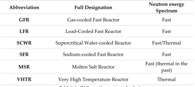
In conclusion, Generation IV reactor should improve safety, sustainability (treatment and disposal of radioactive wastes), economic competitiveness and proliferation resistance. Six different concepts of reactors have been identified by GIF as candidates for further development (Table 1.1).
1 The isotope uranium-238 has been put aside over the years as a by-product of the process where
26
Abbreviation Full Designation Neutron energy
Spectrum
GFR Gas-cooled Fast Reactor Fast
LFR Lead-Cooled Fast Reactor Fast
SCWR Supercritical Water-cooled Reactor Fast/Thermal
SFR Sodium-cooled Fast Reactor Fast
MSR Molten Salt Reactor Fast (thermal in the past)
VHTR Very High Temperature Reactor Thermal
Table 1. 1 - IV Generation reactor technologies
It is worth noting that almost all proposed technologies are based on a fast neutron energy spectrum.
Among the possible FR technologies, SFR is the one with higher accumulated experience, since several prototypes and commercial SFRs operated and operate worldwide [4]. Fig.1.3
summarizes the French experience on SFR reactors.
Fig.1. 3 - French experience on SFR reactors [5]
In France, which is one of the nine original members of the GIF, the first prototype of SFR “Rapsodie” achieved criticality in 1967 in CEA Cadarache Center with a nominal capacity of 20 MWth. The reactor, whose power was increased to 40 MWth for 10 years, operated until April 1983 when it was shut down permanently [5].
27
After this prototype, two commercial SFRs, Phenix and Super-Phenix, operated and were connected to the electrical grid in 1973 and 1986, respectively. Phenix reactor of 250 MWe was built in Marcoule and had a remarkable operational record (final shutdown in 2010). The CEA has acquired an important experience and know-how on sodium fast reactor through Phenix reactor [5].
Differently for Super-Phenix, a 1,242 MWe fast breeder reactor which suffered from a series of cost overruns delays and enormous public protests. Only 15 years after the construction, the reactor reached its design operational goals (1985). The plant was powered down in December 1996 for maintenance, and while it was closed it was subject to court challenges that prevented its restart. In June 1998, Super-Phénix was closed permanently [5].
Fig.1.4 shows the conceptual scheme of sodium pool-type reactors.
Fig.1. 4 - Pool-type Sodium-cooled Fast Reactor [4]
The primary vessel, containing the core, is circulated by liquid sodium, which behaves as coolant. Intermediate heat exchangers (IHX) are also placed in the primary vessel, allowing the primary sodium to exchange thermal power with the secondary loop, also circulated by liquid sodium. The aim of the secondary loop is to avoid any radioactive material outlet from the primary vessel.
28
The secondary loop transfers thermal power from the primary loop to the third one, which is the power conversion cycle. Sodium circulating the first loop is practically at atmospheric pressure, being pressurized at not more than 5 bars. Its core inlet and outlet temperatures are 395°C and 545°C, respectively. The secondary loop is slightly more pressurized than the primary one, in order to avoid primary sodium transfer to the secondary loop in case of leakage.
Concerning the energy conversion cycle, the conventional water Rankine cycle was employed for the French Phenix and Super-Phenix power plants, and for all the others commercial SFRs worldwide. Steam generator design employs water in the tube side (which can be straight or helicoidal) and sodium in the shell side. However, this layout involves a safety issue related to the Sodium-water reaction (SWR) in case of leakage inside the steam generator. Even if the accidental SWR scenario is well managed by the mitigation systems, without safety impact on the reactor, it constituted a weak point considering public acceptance.
1.2. The ASTRID Project
In June 2006, the French government passed a law focused on the disposition of long life high activity waste. An industrial demonstrator, capable of transmutation and separation of long life isotopes, was scheduled for the end of 2020. It was named ASTRID, which stands for “Advanced Sodium Technological Reactor for Industrial Demonstration”. ASTRID project began in 2010 and CEA is in charge of the responsibility for the operational management, core design and R&D work. CEA, along with its industrial partners (French ones: EDF, AREVA etc. and international ones: JAEA, GE, etc.), followed the timetable (Fig.1.5).
29
As already said, ASTRID is the prototype of a GENIV reactor and, as a consequence, it must achieve the requirements established by the GIF.
The major objective, of course, is to build a prototype which can exploit better the natural resources (uranium-238, transuranic) and which can allow to close the fuel cycle (Fig.1.2). In addition, being a prototype, ASTRID has to demonstrate the technological feasibility of sodium fast reactor to electrical energy production, as well as, the sustainable and profitable features from an economic point of view. The choice of the power (600MWe) is reasonable to extrapolate a business plan for future analogous reactors [6].
All these goals must be reached in a structure of improved safety, i.e. [7]:
- Improved core design to lower the probability of core meltdown and/or the energy release following during an accident scenario;
- Better in-service and out-of-service inspection methods and instrumentation;
- Civil structures have to account for mechanical integrity in case of internal or external hazards;
- Three independent shutdown systems; - Innovative gas power conversion system.
One of the most important improvements along with the new core design is the innovative
Energy Conversion System (ECS), which gives a simple and final response to the chemical
reactivity between sodium and water.
It consists in a classical Brayton cycle placed at the tertiary loop of ASTRID reactor layout ending in the turbine generator group producing electrical power, as shown in
Fig.1.6.
30
In this framework the most crucial component to be designed is the sodium-gas heat exchanger (SGHE). In fact, it is responsible for the effective heat transfer from the secondary sodium to the gas that will eventually go through the turbines. Saez et al. [8]
highlight that pumping power has a first order impact on the Brayton cycle efficiency. So, gas circuit total pressure drops have to be minimized: the best estimated compromised between efficiency of the cycle and technological constrains is a sodium/gas heat exchanger pressure drop of 1 bar at maximum on the gas side. This is one of the most important design constraints to be respected.
On the other hand, an electro-magnetic pump (EMP) is used for the circulation of Na in the secondary loop. The power and the sizing of this component (and consequently its impact on the efficiency) are also very sensitive to pressure drops. A design value of 1,5 bar is chosen for the pressure drops of the SGHE Na side.
Being a good compromise between the high thermodynamically efficiency (37.3%) and the R&D effort for the development of gas turbines, the nitrogen gas (N2) is actually the reference option for ASTRID Energy Conversion System (ECS).
1.2.1. The compact Sodium Gas Heat Exchanger (SGHE)
Due to lower heat transfer capacity of nitrogen gas compared to that of boiling water (lower thermal diffusivity α), a significant increase of the heat transfer area is needed. This technical solution would not be admissible in term of fabrication cost, size, and weight if applied to shell and tube heat exchangers. Therefore, compact heat exchanger technology has been chosen for ASTRID Energy Conversion System.
31
Fig.1. 7 – Sodium Gas Heat Exchanger 2014’ design
The sodium/gas heat exchanger is a compact plate counter-flow heat exchanger composed by 8 compact plates modules which are placed in a pressurized vessel at 180 bars (Fig.1.7). Coaxially with the pressure vessel, there is the so-called "shell guide gas". The cold gas flows down from a nozzle to the region between pressure vessel and shell guide gas, then it crosses upward the SGHE modules where the heat exchange takes part. The hot gas flows out from a nozzle at the upper part of the SGHE.
On the other hand, hot sodium enters in the exchanger from the bottom part, but it flows across SGHE module downward. In fact, the Na pipes inside the pressure vessel bring the Na at the top of the module. This configuration allows the counter-flow exchange. The cold sodium is then collected in pipes at the bottom part of the structures.
32
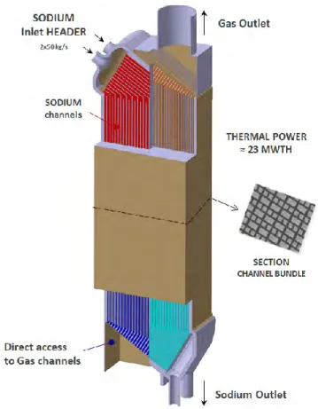
Fig.1. 8 - SGHE Module
The SGHE half module consists of a stack of 72 Na channels layers intercalated with 72 gas channel layers. Each Na layer is constituted by 125 sodium channels which means that a total of 9000 rectangular sodium channels, with a 3 x 6 mm2 cross section and a length around 2.2 m, have to be fed. This configuration is required to achieve the thermal-mechanical performance of the heat exchanger module (23.4 MWth).
On sodium side, 100kg/s mass flow rate supplies the vast number of parallel channels through two admission pipes which are also placed into the pressure vessel, subjected to 180 bars of external pressure at a temperature of 530 ° C (Fig.1.6). Their diameter of 90mm is the compromise between the mechanical resistance of the admission pipe and hydraulic requirements concerning the cavitation risk and pressure drops (inlet sodium velocity < 10m/s).
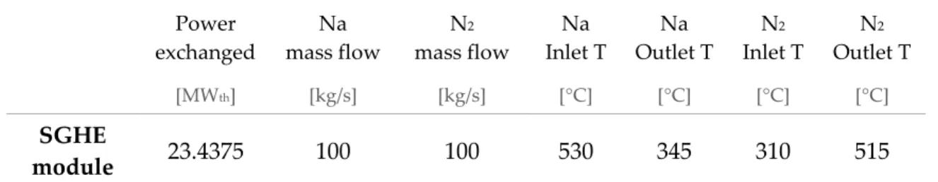
33 Power exchanged Na mass flow N2 mass flow Na Inlet T Na Outlet T N2 Inlet T N2 Outlet T [MWth] [kg/s] [kg/s] [°C] [°C] [°C] [°C] SGHE module 23.4375 100 100 530 345 310 515
Table 1. 2 – SGHE module thermos-hydraulic features
Note that, the design of the module and the arrangement of the pipes in Fig.1.7 are currently under further investigation, but even if some details can be changed the conceptual design is now consolidated.
1.3. Scope of the work
The SGHE design proposed by the CEA involves important benefits for the project. For instance, the minor pressure drops in gas-side comparing other design solutions tested, the optimization of thermomechanical stresses and the minimization of the Na inventory (8 m3) are surely some of the most important [9].
However, one critical problem occurs in the sodium side, i.e. the flow “maldistribution”. As the prefix mal suggests, flow maldistribution denotes a defective distribution of mass flow rate between parallel channels of the HE.
The description of SGHE module in Section 1.2.1 makes already evident some geometrical features and flow conditions which inevitably lead to a serious problem of flow maldistribution, i.e. the high dynamic pressure at the inlet (𝑣𝑖𝑛𝑙𝑒𝑡 = 10 𝑚/𝑠) and the low
pressure drop of the large bundle (minimal required channel cross-section). All maldistribution causes are discussed in detail in Section 2.4.1.
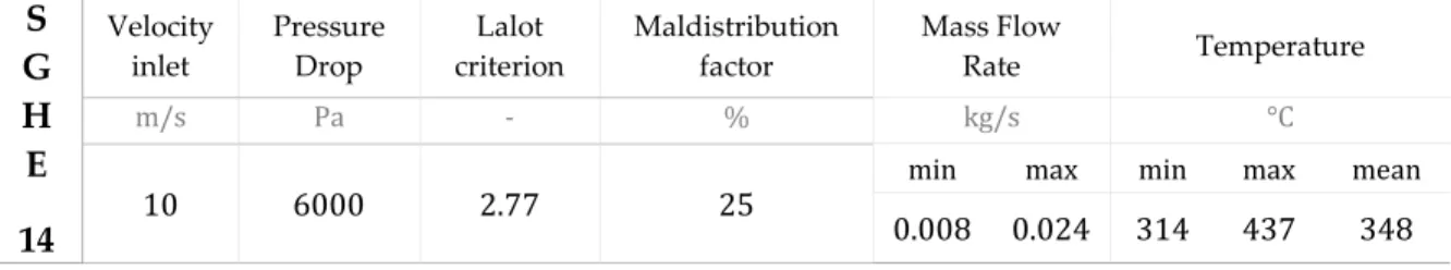
The maldistribution factor2 𝜎 associated to the present SGHE design is estimated to 25 %.
The deriving temperature variation between sodium channels generates internal thermal stress and thus deformation of structure. As conclusion, the current design of the SGHE
2In the present work, the flow maldistribution will be evaluated using the following factor, based on standard
deviation:
𝜎 =
√∑ (𝑚𝑁𝑖 ̇ − 𝑚̇𝑖 ̅ )2
𝑁
𝑚̇̅ 𝑥100 (1)
where 𝑚̇𝑖 is the mass flowrate in a channel; 𝑚̇̅ the average mass flowrate of the whole channels and 𝑁 is the
34
module is not attainable since thermo-mechanical stresses are not allowable (higher than 200 MPa).
Therefore, the scope of the present work consists in studying the ‘maldistribution’ in compact heat exchangers, in order to identify possible design solutions and to understand the physical phenomena providing flow maldistribution conditions. The physical understanding will be used to determine the research patterns that will be followed in this PhD work to increase the SGHE performance and to provide validated tools to correctly study the ‘maldistribution’ issue.
1.4. Thesis Outline
After this brief introduction to the issue of flow ‘maldistribution’ in ASTRID Sodium-Gas heat exchanger, the entire PhD work will give out as in the following:
- A bibliographic overview on different types of flow distributor commonly used in industrial applications will be exhibited in Chapter 2. The study offers the possibility to explore flow performance under various geometries suggesting the configuration best suited to meet ASTRID Sodium-Gas heat exchanger requirements. An innovative homogenization system will be presented.
- Chapter 3 will describe the two experimental facilities used in the present work; one is dedicated to the investigation of sodium flow in pre-distribution channels and the other to the study of flow behavior in the integral geometry of the SGHE module. The experimental database will be useful to actually validate the numerical models.
- The numerical approach and turbulence model selected to study the flow in pre-distribution bifurcating channels will be presented in Chapter 4. Numerical and experimental results will be shown together. Once the model is validated, a design optimization will be provided, showing the optimal solution for sodium pre-distribution channels in ASTRID SGHE module.
- Chapter 5 deals with the study of the global flow ‘maldistribution’ between sodium channels in the SGHE module. Numerical results will be compared with the experimental data collected during the second experimental campaign. The validated numerical model will be used to propose a final SGHE design of sodium header and pre-distribution channels allowing a uniform flow distribution.
35
36
Chapter 2
Bibliographic Study
Maldistribution of flow is a key topic for efficiency and operability of heat exchangers. A great number of theoretical models and experimental studies can be found in the context of flow distribution in heat exchangers. Three different types of flow headers commonly used in industrial applications are considered in this work, i.e. consecutive manifold, normal-flow header and bifurcation manifold. Their analysis offers the possibility to explore flow distribution performance under various geometries suggesting the configuration best suited to ASTRID Sodium-Gas heat exchanger requirements.
In Section 2.1, the interest in studying flow distribution in the simple geometry of consecutive manifolds stems from the fact that generalized equations of analytical models allow to easily identify key factors influencing flow maldistribution. However, most of existing works based their formulations on assumptions ignoring some complex and important physical aspects for ASTRID project.
Other authors developed computational models and experimental investigations to predict flow distribution in bifurcation manifolds and normal-flow headers (Section 2.2
and Section 2.3). Generalized recommendations for preventing the negative consequences of flow maldistribution and some improved configurations are presented giving some suggestions for SGHE design. However, due to many geometrical variations and lack of any available theory, previous studies are not sufficient to asses an optimized design for ASTRID heat exchanger.
Most problems must be solved by intelligent design and diagnosis on an individual basis. In this sense, the last section will expose how the main findings and conclusions of the bibliographic study delineate the strategy to improve flow maldistribution in ASTRID heat exchanger (Section 2.4).
Before describing all various types of flow distributors and the associated experimental and modeling studies, let us focus the attention on the general maldistribution problem in compact heat exchanger technologies.
37
Flow Maldistribution in Compact Heat Exchanger
Compact heat exchangers are characterized by a large heat transfer surface area to volume ratio. This permits a great deal of heat transfer to take place between streams in a very small volume and with very small driving temperature differences. However, a large heat transfer surface embodied in a small volume will require a vast number of small channels for making effective use of the available primary and secondary surface.
Starting from the conceptual design of compact HE illustrated in Fig.2.1, the inherent difficulties in providing the uniform flow distribution are clear to understand.
Fig.2. 1 – Compact heat exchanger – Inlet Header [12]
First of all, the flow passages of small size are certainly susceptible to imperfect manufacturing processes. Therefore, fabrication and manufacturing tolerances may result in unacceptably poor performances of the heat exchanger3[11].
The second problem is mainly related to the inlet flow conditions. The inlet stream flow is admitted thorough a small port compared to the large surface of the heat exchanger core (bundle channel). As a consequence, a stream jet occurs in the inlet flow distributor resulting in a non-uniform distribution between channels of the core. In addition, the shape of inlet flow distributor could produce high-velocity regions leading to localized erosions at the core face as well as unallowable thermo-mechanical loads [11].
3 The proper distribution of uniform flow distribution is essential to achieve the required thermal
performance. In fact, the flow non-uniformity may result in performance deterioration and may affect the mechanical integrity of the compact heat exchanger.
38
The magnitude of these effects strongly depends on the design of the fluid distribution elements connecting the heat exchanger core and the inlet and outlet fluid flow lines. Their modeling is actually very important to predict the impact on heat exchanger performance.
2.1. Consecutive Manifold
A consecutive manifold is one of the most commonly structures used for the distribution of fluid stream in compact heat exchangers. It consists in a flow channel for which fluid enters or leaves through a multiple sidewall outlet. Basic types of flow manifold are illustrated in Fig.2.2. In dividing-flow manifolds (a), fluid enters laterally and exits the manifold axially. Inversely, in combining-flow manifolds (b). When interconnected by lateral branches, these manifolds result in parallel (c) and reverse-flow systems (d), or U- and Z-flow arrangements.
Fig.2. 2 - Major types of manifolds [12]
This type of distributor [12] is widely used in many industrial applications due to their clear advantages of simplicity. This means low development cost and time-efficient design for the manufacturing cycle. Furthermore, available explicit analytical solutions based on differential equations enable the development of generalized methods correlating flow distribution performance and manifold structure, i.e. an easy-to-use guidance for manifold designers.
The object of a consecutive manifold is to provide an equal distribution of flow through the multiple side openings. This is essentially prevented from the variation of pressure field along the main channel. In fact, in a dividing flow header, the main fluid stream is decelerated due to the loss of fluid through side openings and flow pressure rises in the direction of flow (fluid-momentum effect) (Fig.2.3c-d) [12]. However, in the main channel, also named header, the effect of fluid friction against the internal surface of main channel can make pressure falls in the direction of flow (friction effect). This means that a uniform
39
pressure along the dividing flow header can be obtained by a suitable adjustment of the flow parameters; the pressure regaining due to flow branching balances the pressure losses due to friction.
Fig.2. 3 - Manifold configurations: (a) U-flow or parallel flow configuration; (b) Z-flow or reverse-flow configuration. Pressure profile in (c) U-flow configuration, (d) Z-flow configuration [12]
It is worth noting that as shown in Fig.2.3c, for parallel manifold the friction and momentum effect work in opposite direction, the first tending to produce a pressure drop and the second a pressure rise. For reverse manifold, both friction and moment effect tend to create a lower pressure at the open and the closed end of manifold (Fig.2.3d).
To identify geometrical and physical parameters providing the suitable adjustment of fluid-momentum and friction effect in consecutive manifolds, various theoretical, experimental and numerical studies have been proposed in the past and they are presented below.
2.1.1. Theoretical studies of flow manifold
The simplicity of the analytical approach used to study consecutive manifolds allows to easily identify some relevant parameters influencing flow distribution such as cross-sectional area of all lateral channels 𝐴𝑐, header cross-sectional area 𝐴 ( 𝐴𝑖 for the intake
header and 𝐴𝑒 for the exhaust header), header length L, and the resistance of lateral
40
Fig.2. 4 – Geometrical parameters influencing flow distribution [20]
However, the weakness of theoretical models of flow manifold is related to the generalization of analytical solutions. In fact, despite their good description of the physics, analytical solutions are usually valid only for specific manifolds and flow conditions. For sake of clarity, in the following section we will examine the development of some significant analytical solutions of continuous models [12-20]. Special attention will be paid to the theoretical approach chosen to represent the branching process.
In presenting flow modeling of different authors, a U-type arrangement of flow manifold constructed from a main channel of constant cross-sectional area (𝐴) and equally spaced channels of uniform size is selected as general computational domain (Fig.2.5).
Fig.2. 5 - Schematic diagram of U-Type manifold [20]
Control volumes describing the flow streams near a dividing and combining flow branch point are illustrated in Fig.2.6.
41
Fig.2. 6 - Control volume for intake (a) and exhaust (b) header [20-21]
Acrivos et al. [13] analyzed the performance of a simple dividing manifold (Fig.2.6a) by applying a momentum equation along the main channel. To represent the pressure recovery phenomena, they modified Bernoulli equation by introducing a correction term of momentum. The correction term was determined experimentally from observed pressure changes in near a single outlet port [13].
In their model, they essentially related the pressure variation to the momentum changes in the main flow stream (momentum effect) and the fractional losses based on the local flow spread (friction effect).
The resulting nonlinear, second-order, ordinary differential equation is written as: 𝑑𝑃 𝑑𝑋+ 𝑊̅ 𝑑𝑊̅ 𝑑𝑥 + 𝐹0𝑊̅ 7 4= 0 (2)
where 𝑃, 𝑊 and X are the axial pressure, the velocity and the coordinate of manifold. 𝐹0 represents the combination of the friction and the pressure recovery effects.
Nevertheless, Acrivos’ model could not be considered as a general analytical solution for flow in manifold. First of all, for the straight-tube section of manifold they assume that the friction factor varies with fluid flow velocity of the power of -1/4 which limits the applicability of the model for Blasius’ flows. Secondly, the combination of the friction and the pressure recovery factors complicates the understanding of mutual interaction between the two effects. In addition, the model had been applied only to the case of simple dividing manifolds.
It’s worth noting that in the above theoretical model, the effects of axial momentum transport by the lateral fluid stream (𝑈𝑐 in Fig.2.6a) are not considered.
To overcome this problem, Bajura and Jones [14-15] integrated, for the first time, a discharge equation for lateral flow in super-heated power plant boilers. The overall mass and momentum balance can be resolved for the whole control volume (Fig.2.6a-b) and the
42
effects of the branching process are directly included in the analysis. Bassiouny and Martin extended the model for plate fin-heat exchangers [16-17].
The resulting differential equation for the velocity in the intake header is written as: 1 𝜌 𝑑(𝑃𝑖− 𝑃𝑒) 𝑑𝑋 + 1 2[ 𝑓𝑖 𝐷𝑖 + 𝑓𝑒 𝐷𝑒 (𝐴𝑖 𝐴𝑒 ) 2 ] 𝑊𝑖2− [(2 − 𝛽𝑒) ( 𝐴𝑖 𝐴𝑒 ) 2 − (2 − 𝛽𝑖)] 𝑊𝑖 𝑑𝑊𝑖 𝑑𝑋 = 0 (3) where 𝐴, 𝐷 and P are the cross-sectional area, the diameter and the axial pressure of manifold. The term 𝛽 represents the fraction of axial velocity 𝑊𝑖 that will be branched off
through the main channel (𝑊𝑐 = 𝛽𝑊𝑖). Subscripts i and e refer to intake and exhaust
headers.
In equation (3), the second term in the left hand of the equation represents the friction contribution to the pressure drop in lateral channels and the third term the momentum contribution due to the flow branching in the channels.
However, both Bassionuy and Martin [16-17] and Bajura and Jones [14-15] provided an analytical solution of equation after neglecting the frictional term. For plate fin-heat exchangers, the friction loss in the main channel can be effectively neglected compared to the pressure drop in lateral channels and the momentum change due to the branching process. The analytical solution is then valid only for short manifolds where friction effects are negligible small compared to momentum effects.
On the other hand, Maharuadraya et al. [18] retained the frictional term but neglected the inertial term. The solution of equation (3) is valid only for long manifolds, where the frictional effects dominate. In addition, the first limitation of Acrivos’ model remains in both models.
As conclusion, despite a good description of the physics, the above presented models present limits for designing manifold system with uniform flow distribution. In fact, an isolated adjustment of pressure-recovery effect or friction effect could result in the failure of uniform design.
Only in 2010, the first general analytical solution of governing equation (3) for flow distribution in U-type arrangement manifold has been provided by Wang et al. [19-20]. Both the frictional and momentum term are finally taken into account in their solution. The explicit expression of the analytical solution allows manifold designers to easily identify key factors influencing flow maldistribution [21].
43
Flow area ratio, 𝑀
Flow area ratio 𝑀 is defined as the ratio of the total cross-sectional area of all lateral channels (N𝐴𝑐) to the header cross-sectional area (𝐴). Wang et al. [19] show in Fig.2.7 that
a uniform flow distribution can be obtained when M is smaller. For a larger M, the momentum cannot balance friction effect. Bajura and Jones [6] suggest M< 1 for the manifold system design.
𝑉𝑐, in Fig.2.7, corresponds to the dimensionless volume flow rate flowing in each port of
the consecutive manifold.
Fig.2. 7 –Effect of flow area ration M on flow distribution [19] Ratio of header length to diameter, 𝐸
𝐸 is defined as the ratio of the total length of header (L) to the diameter (D). For a larger E, a less uniform distribution occurs (Fig.2.8). In fact, friction resistance increases along the manifold and more momentum is needed. Varying only this parameter it would be difficult to improve flow distribution. Wang et al. [19] also demonstrated that a ratio E < 5 has not a significant impact on flow distribution.
44
Flow resistance in lateral channels, 𝜉
The total pressure loss coefficient of lateral channels 𝜉 has a decisive impact on flow distribution. A more uniform distribution may be reached for a higher resistance of lateral channels (Fig.2.9). For an infinite value of 𝜉, the manifold will act as a closed system and an absolute uniform distribution can be reached. However, for 𝜉 > 5, there is not a remarkably improvement of flow distribution [19].
Fig.2. 9 - Effect of flow resistance in lateral channels ξ on flow distribution [19] Inlet Reynold Number or entrance effect
A high inlet Reynolds number implies an increase of pressure drop along the manifold (friction effect) leading a less uniform distribution.
However, when E is smaller, the influence of inlet Reynolds Number can be neglected. In fact, as demonstrated by Bassiouny et al. [16-17], in short manifolds the momentum effect is predominant and the friction term can be neglected.
Flow direction
Datta and Majumdar [18] studied the influence of flow direction in intake or exhaust headers on flow distribution. They demonstrate that, for the same flow area ratio, U-type arrangement manifold provides a more uniform distribution than Z-type. This could be explained by the more uniform distribution of pressure difference between two headers for U-type manifold systems (Fig.2.3 c).
As conclusion, the present section demonstrated how one-dimensional analytical numerical model can represent a suitable tool for the optimization of manifold geometry and the preliminary design.
![Table 2. 1 - Flow maldistribution: PIV results [29], CFD Wen [29] et al. and CFD Raul et al [34]](https://thumb-eu.123doks.com/thumbv2/123doknet/3055501.86230/59.918.134.767.133.317/table-flow-maldistribution-piv-results-cfd-wen-raul.webp)
![Table 2. 2 - Characteristics of flow distributor Circular-321 [41]](https://thumb-eu.123doks.com/thumbv2/123doknet/3055501.86230/65.918.455.795.645.779/table-characteristics-flow-distributor-circular.webp)