PeRL: a circum-Arctic Permafrost Region Pond and Lake database.

(1)

https://doi.org/10.5194/essd-9-317-2017 © Author(s) 2017. This work is distributed under the Creative Commons Attribution 3.0 License.

PeRL: a circum-Arctic Permafrost Region Pond

and Lake database

Sina Muster1, Kurt Roth2, Moritz Langer3, Stephan Lange1, Fabio Cresto Aleina4, Annett Bartsch5, Anne Morgenstern1, Guido Grosse1, Benjamin Jones6, A. Britta K. Sannel7, Ylva Sjöberg7,

Frank Günther1, Christian Andresen8, Alexandra Veremeeva9, Prajna R. Lindgren10,

Frédéric Bouchard11,13, Mark J. Lara12, Daniel Fortier13, Simon Charbonneau13, Tarmo A. Virtanen14, Gustaf Hugelius7, Juri Palmtag7, Matthias B. Siewert7, William J. Riley15, Charles D. Koven15, and

Julia Boike1

1_{Alfred Wegener Institute Helmholtz Centre for Polar and Marine Research, Telegrafenberg A43,} 14473 Potsdam, Germany

2_{Institute for Environmental Physics, Heidelberg University, Heidelberg, Germany} 3_{Humboldt University, Berlin, Germany}

4_{Max Planck Institute for Meteorology, Hamburg, Germany} 5_{Zentralanstalt für Meteorologie and Geodynamik, Vienna, Austria} 6_{U.S. Geological Survey – Alaska Science Center, Anchorage, AK 99508, USA}

7_{Stockholm University, Department of Physical Geography and the Bolin Centre for Climate Research,} 10691 Stockholm, Sweden

8_{Los Alamos National Laboratory, Los Alamos, NM, USA}

9_{Institute of Physicochemical and Biological Problems in Soil Science, Russian Academy of Sciences,} Pushchino, Russia

10_{Geophysical Institute, University of Alaska Fairbanks, Fairbanks, AK, USA}

11_{Institut national de la recherche scientifique (INRS), Centre Eau Terre Environnement (ETE), Québec QC,} G1K 9A9, Canada

12_{Department of Plant Biology, University of Illinois at Urbana-Champaign, Urbana, IL 61801, USA} 13_{Geography Department, University of Montréal, Montréal QC, H3C 3J7, Canada}

14_{Department of Environmental Sciences, University of Helsinki, Helsinki, Finland}

15_{Climate and Ecosystem Sciences Division, Lawrence Berkeley National Laboratory, Berkeley, USA} Correspondence to:Sina Muster ([email protected])

Received: 15 November 2016 – Discussion started: 22 November 2016 Revised: 27 March 2017 – Accepted: 1 April 2017 – Published: 6 June 2017

Abstract. Ponds and lakes are abundant in Arctic permafrost lowlands. They play an important role in Arctic

wetland ecosystems by regulating carbon, water, and energy fluxes and providing freshwater habitats. However, ponds, i.e., waterbodies with surface areas smaller than 1.0 × 104m2, have not been inventoried on global and regional scales. The Permafrost Region Pond and Lake (PeRL) database presents the results of a circum-Arctic effort to map ponds and lakes from modern (2002–2013) high-resolution aerial and satellite imagery with a reso-lution of 5 m or better. The database also includes historical imagery from 1948 to 1965 with a resoreso-lution of 6 m or better. PeRL includes 69 maps covering a wide range of environmental conditions from tundra to boreal re-gions and from continuous to discontinuous permafrost zones. Waterbody maps are linked to regional permafrost landscape maps which provide information on permafrost extent, ground ice volume, geology, and lithology. This paper describes waterbody classification and accuracy, and presents statistics of waterbody distribution for each site. Maps of permafrost landscapes in Alaska, Canada, and Russia are used to extrapolate waterbody statis-tics from the site level to regional landscape units. PeRL presents pond and lake estimates for a total area of

(2)

1.4 × 106km2across the Arctic, about 17 % of the Arctic lowland (< 300 m a.s.l.) land surface area. PeRL wa-terbodies with sizes of 1.0 × 106m2 _{down to 1.0 × 10}2_m2_{contributed up to 21 % to the total water fraction.} Waterbody density ranged from 1.0 × 10 to 9.4 × 101km−2. Ponds are the dominant waterbody type by number in all landscapes representing 45–99 % of the total waterbody number. The implementation of PeRL size distri-butions in land surface models will greatly improve the investigation and projection of surface inundation and carbon fluxes in permafrost lowlands. Waterbody maps, study area boundaries, and maps of regional permafrost landscapes including detailed metadata are available at https://doi.pangaea.de/10.1594/PANGAEA.868349.

1 Introduction

Globally, Arctic lowlands underlain by permafrost have both the highest number and area fraction of waterbodies (Lehner and Döll, 2004; Grosse et al., 2013; Verpoorter et al., 2014). These landscapes play a key role as a freshwater resource, as habitat for wildlife, and as part of the water, carbon, and energy cycles (Rautio et al., 2011; CAFF, 2013). The rapid warming of the Arctic affects the distribution of surface and subsurface water due to permafrost degradation and in-creased evapotranspiration (Hinzman et al., 2013). Remote-sensing studies have found both increasing and decreasing trends in surface water extent for waterbodies in permafrost regions across broad spatial and temporal scales (e.g., Carroll et al., 2011; Watts et al., 2012; Boike et al., 2016; Kravtsova and Rodionova, 2016). These studies, however, are limited in their assessment of changes in surface inundation since they only include lakes, i.e., waterbodies with a surface area of 1.0×104m2or larger. Ponds with a surface area smaller than 1.0×104m2, on the other hand, have not yet been inventoried on the global scale. Yet ponds dominate the total number of waterbodies in Arctic lowlands, accounting for up to 95 % of individual waterbodies, and may contribute up to 30 % to the total water surface area (Muster et al., 2012; Muster, 2013). Arctic ponds are characterized by intense biogeophys-ical and biogeochembiogeophys-ical processes. They have been identi-fied as a large source of carbon fluxes compared to the sur-rounding terrestrial environment (Rautio et al., 2011; Laurion et al., 2010; Abnizova et al., 2012; Langer et al., 2015; Wik et al., 2016; Bouchard et al., 2015). Due to their small sur-face areas and shallow depths, ponds are especially prone to change; various studies reported ponds drying out or increas-ing in abundance due to new thermokarst or the drainage of large lakes (Jones et al., 2011; Andresen and Lougheed, 2015; Liljedahl et al., 2016). Such changes in surface in-undation may significantly alter regional water, energy, and carbon fluxes (Watts et al., 2014; Lara et al., 2015). Both the monitoring and modeling of pond and lake development are therefore crucial to better understand the trajectories of Arctic land cover dynamics in relation to climate and en-vironmental change. Currently, however, the direction and magnitude of these changes remain uncertain, mainly due to the limited extent of high-resolution studies and the lack of pond representation in global databases. Although recent

ef-forts have produced global land cover maps with resolutions of 30 m (Liao et al., 2014; Verpoorter et al., 2014; Feng et al., 2015; Paltan et al., 2015), these data sets only include lakes.

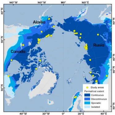
To complement previous approaches, we present the Per-mafrost Region Pond and Lake (PeRL) database, a circum-Arctic effort that compiles 69 maps of ponds and lakes from remote-sensing data with high spatial resolution (of ≤6 m) (Fig. 1). This database fills the gap in available global databases that have cutoffs in waterbody surface area at 1.0 × 104m2or above. In addition, we link PeRL waterbody maps with existing maps of permafrost landscapes to extrap-olate waterbody distributions from the individual study areas to larger landscapes units. Permafrost landscapes are terrain units characterized by distinct properties such as climate, sur-ficial geology, parent material, permafrost extent, ground ice content, and topography. These properties have been iden-tified as major factors in the evolution and distribution of northern waterbodies (Smith et al., 2007; Grosse et al., 2013; Veremeeva and Glushkova, 2016).

The core objectives of the PeRL database are to (i) archive and disseminate fine-resolution geospatial data of northern high-latitude waterbodies, (ii) quantify the intra- and in-terregional variability in waterbody size distributions, and (iii) provide regional key statistics, including the uncertainty in waterbody distributions, that can be used to benchmark site-, regional-, and global-scale land models.

2 Definition of ponds and lakes

The definition of ponds and lakes varies in the literature and depends on the chosen scale and goal of studies when charac-terizing waterbodies. The Ramsar classification scheme de-fines ponds as permanently inundated basins smaller than 8.0×104m2in surface area (Ramsar Convention Secretariat, 2010). Studies have also used surface areas smaller than 5.0×104m2(Labrecque et al., 2009) or 1.0×104m2(Rautio et al., 2011) to distinguish ponds from lakes.

In remote-sensing studies, surface area is the most reliably inferred parameter related to waterbody properties. Physical and biogeochemical processes of waterbodies, however, also strongly depend on waterbody depth. Differences in ther-modynamics are associated with water depth, where deeper lakes may develop a stratified water column while shallow

(3)

Figure 1.Distribution of PeRL study areas. Permafrost extent ac-cording to Brown et al. (1998).

ponds remain well mixed. In high latitudes, waterbodies with depths greater than 2 m are likely to remain unfrozen at the bottom throughout winter, thus providing overwinter-ing habitat for fish and other aquatic species. In permafrost regions, a continuously unfrozen layer (talik) may develop underneath such deeper waterbodies, which strongly affects carbon cycling in these sediments (Schuur et al., 2008). Sev-eral studies have shown a positive correlation between wa-terbody surface area and depth (Langer et al., 2015; Wik et al., 2016). However, there is large variability in the area– depth relationship, i.e., there are large but shallow lakes that freeze to the bottom and small but deep ponds that develop a talik, and these characteristics may also change over time with changes in water level and basin morphology. In this study we distinguish ponds and lakes based on their surface area. We adopt the distinction of Rautio et al. (2011) and de-fine ponds as bodies of largely standing water with a surface area smaller than 1.0 × 104m2and lakes as waterbodies with a surface area of 1.0 × 104m2or larger.

3 PeRL database generation

3.1 Data sources and processing

PeRL’s goal is to make high-resolution waterbody maps available to a large science community. PeRL compiles both previously published and unpublished fine-scale waterbody maps. Maps were included if they met the resolution crite-ria of 5 m or less for modern imagery and 6 m for

histori-cal imagery. Historihistori-cal imagery was included to enable high-resolution change detection in ponds and lakes.

Twenty-nine maps were specifically produced for PeRL to complement the published maps in order to represent a broad range of landscape types with regard to permafrost extent, ground ice content, geology, and ecozone. All waterbody maps were derived from optical or radar airborne or satellite imagery that were acquired between mid and late summer (July–September), thereby excluding the snowmelt and early summer season. Modern imagery dates from 2002 to 2013, and historical imagery dates from 1948 to 1965. Previously published maps are the product of many independent studies, which leads to a broad range of image types and classification methods used. Details on image processing and classification procedures for already published maps (n = 31) are listed in Table A1 and the respective publications. The processing of new PeRL maps is described in Sect. 3.2.

3.2 PeRL image processing and classification 3.2.1 Image processing

Available high-resolution imagery used for PeRL map pro-duction included optical aerial and satellite imagery (Geo-Eye, QuickBird, WorldView-1 and -2, and the Korean Multi-Purpose Satellite 2 (KOMPSAT-2)) and radar (TerraSAR-X) imagery.

Most optical imagery provided a near-infrared band that was used for classification, with the exception of World-View 1, which only has a panchromatic band. Preprocessing of the optical imagery involved georeferencing or orthorecti-fication depending on the availability of high-resolution dig-ital elevation models (Appendix A, Table A1).

TerraSAR-X (TSX) imagery was acquired in Stripmap Mode with an HH polarization as the geocoded Enhanced El-lipsoid Corrected (EEC) product or as the Single Look Slant Range Complex (SSC) product which was then processed to EEC (Sect. A1). TSX images were filtered in ENvironment for Visualizing Images (ENVI) v4.7 (ITTVIS) in order to re-duce image noise using a lee filter with a 3 × 3 pixel window followed by a gamma filter with a 7 × 7 or 11 × 11 window depending on the image quality (Klonus and Ehlers, 2008).

3.2.2 Classification of open water

Imagery was classified using either a density slice or an unsu-pervised k-means classification in ENVI v4.8 (ITTVIS). The panchromatic, the near-infrared, and the X-Band (HH polar-ization) show a sharp contrast between open water and sur-rounding vegetation. Visual inspection of the imagery could therefore be used to determine individual threshold values (in the case of density slice) or to assign classes (in the case of k-means unsupervised classification) for the extraction of open-water surfaces. Threshold values and class boundaries varied between images and sites due to differences in illu-mination, acquisition geometry, and radiometric properties

(4)

of images. Detailed information on remote-sensing imagery and the classification procedure for each site is listed in Ap-pendix A (Table A1).

The classification procedure in ENVI produces raster im-ages that were converted to ESRI vector files so that each waterbody is represented as a single polygon. Vector files were then manually processed in ArcGIS v10.2 (ESRI) to fill gaps in waterbody surfaces and remove streams, rivers, and shadows due to clouds or topography and partial lakes along the study area boundaries. The minimum waterbody size was set to at least 4 pixels. This equals less than 4 m2 for the highest resolutions of less than 1 m and 64 m2for the lowest resolution of 4 m for modern imagery (1.4 × 102m2 for historical imagery with resolutions of 6 m). All classified objects smaller than the minimum size were removed. Partial lakes along the study area boundaries, segments of streams and rivers, and shadows due to clouds or topography were manually removed.

3.3 Study area boundaries

Each waterbody map is associated with a vector file that de-lineates the study area’s boundary. Boundaries were calcu-lated for each map – whether new or previously published – in ArcGIS by first producing a positive buffer of 1–3 km around each waterbody in the map and merging the individ-ual buffers into one single polygon. From that single polygon we then subtracted the same distance again, which rendered the study area boundary. The area of the boundary is referred to as the total mapped extent of that site (Table 1). For sites with multi-temporal data, the total mapped extent of the old-est classification was chosen as a reference in order to calcu-late changes in pond and lake statistics over time.

4 PeRL statistical analysis

Statistics such as areal fraction of water or average water-body surface area are meaningful measures to compare wa-terbody distributions between individual study areas and per-mafrost landscapes. Statistics were calculated for all water-bodies, as well as separately for ponds and lakes. We cal-culated areal fraction, i.e., the area fraction of water relative to land (the total mapped area), and waterbody density, i.e., the number of waterbodies per kilometer for each site, using the software package R version 3.3.1. However, statistics are subject to the size of the study area. Very small study areas may not capture larger waterbodies, which may nonetheless be characteristic of the larger landscape. Very large study ar-eas, on the other hand, may show more spatial variation in waterbody distribution than smaller study areas. In order to make statistics comparable between study areas, we subdi-vided larger study areas into boxes of 10 km×10 km. The box size was chosen as a function of the standard error (Sect. A2). We calculated the statistics for each box and then averaged the statistics across all boxes within each study area. This

subgrid analysis was conducted for all study areas larger than 300 km2for which at least four boxes could be sampled.

Statistics are also subject to image resolution, which defines the minimum object size that can be confidently mapped. For all modern imagery, the minimum waterbody size included in the calculation of statistics was therefore set to 1.0 × 102m2(1.4 × 102m2 for historical imagery). Very large lakes are not representative of all study areas and may only be partially mapped within a 10 km × 10 km box. We therefore chose a maximum waterbody size of 1.0 × 106m2 to be included in the calculation of statistics.

5 Extrapolation of site-level waterbody statistics to

permafrost landscapes

5.1 Regional maps of permafrost landscapes

Waterbody statistics of each site were extrapolated to per-mafrost landscapes based on the assumption that distribu-tions of ponds and lakes are similar for similar permafrost landscapes, i.e., areas with similar properties regarding cli-mate, geology, lithology (soil texture), permafrost extent, and ground ice volume. Vector maps of permafrost land-scapes (PLM) are available on the regional level: the Alaskan map of permafrost characteristics (AK2008) (Jorgenson et al., 2008a), the National Ecological Framework for Canada (NEF) (Marshall et al., 1999), and the Land Resources of Russia (LRR) (Stolbovoi and McCallum, 2002). Despite differences in mapping approaches and terminology, these databases report similar landscape characteristics on compa-rable scales. All regional maps were available as vector files, which were converted to a common North Pole Lambert Az-imuthal Equal-Area (NPLAEA) projection. All PLM were clipped in ArcGIS v10.4 with a lowland mask including only areas with elevations of 300 m or lower. The lowland mask was derived for the entire Arctic using the digital elevation model GTOPO30 (USGS). Details on the properties of each PLM are provided in Appendix B. The original PLM were merged in ArcGIS to produce a unified circum-Arctic vector file and map representation. Landscape attributes that were retained from the original PLM were ecozone, permafrost extent, ground ice volume, surficial geology, and lithology. Variable names were consolidated using uniform variable names (Appendix B, Table B4).

5.2 Extrapolation of waterbody statistics to permafrost landscapes

Waterbody maps were spatially linked with their associated permafrost landscape. Maps within the same landscape were combined, whereas maps spanning two or more landscapes were divided by selecting all waterbodies that intersected with the respective permafrost landscape. If several maps were present within one permafrost landscape unit they were combined and average statistics calculated across all maps in

(5)

that unit. Historical maps and unedited classifications were not used in the extrapolation.

Extrapolations were done in Alaska, Canada, and Russia for waterbody maps with a (combined) extent of 100 km2or larger but not for Europe where available waterbody maps were too small. Maps in the Canadian high Arctic were smaller than 1.0 × 102km2but represent typical wetlands in that region and were therefore included in the extrapolation. Figures D1, D2, D3, and D4 show the location of waterbody maps within their associated permafrost landscape.

Extrapolated statistics were assigned two confidence classes: (1) high and (2) low confidence. Permafrost land-scapes were assigned to the high confidence class if a map was present in the permafrost landscape of that ecozone. The low confidence class indicates that statistics were derived from the same permafrost landscape but in a different eco-zone. Due to differences in the mapping and generalization of landscape properties of the regional PLM, the extrapola-tion was conducted only within each region.

6 PeRL database features

The database provides two different map products: (i) site-level waterbody maps and (ii) an extrapolated circum-Arctic waterbody map. The database also provides different tables which present statistical parameters for each individual wa-terbody map (Appendix B) and aggregated statistics for per-mafrost landscape (PL) units in the circum-Arctic map (Ta-ble 3).

6.1 Site-level waterbody maps 6.1.1 Data set structure

Altogether, the database features 70 individual waterbody maps as ESRI shape files. Each waterbody shape file is named according to a map ID. The map ID consists of a three-letter abbreviation of the site name, followed by a run-ning three-digit number and the acquisition date of the base imagery (YYYY-MM-DD). Vector files were projected to the NPLAEA projection. The area and perimeter of each water-body and site were calculated in ArcGIS 10.4 in square me-ters. Each vector file is accompanied by an xml-file which lists metadata about classification and references as pre-sented in Tables 1 and A1. Each map has a polygon asso-ciated with it that contains the study area, i.e., the total land area of the waterbody map. All study area boundaries are stored in the file PeRL_study_areas.shp and can be identified via the map ID (Table C2). The study area shape file also includes the site characteristics listed in Table 2.

Fifty-eight maps are considered “clean”, i.e., they have been manually edited to include only ponds and lakes (Ta-ble 1). Eight maps are “clean with partial waterbodies”. These are multi-temporal maps with very small map ex-tents where partial waterbodies along the study area

bound-101 ₁₀3 ₁₀5 ₁₀7 0 20 40 60 80 100 Cu m u la ti v e f ra c ti o n o f w a te rb o d y a re a [ % ]

log10 (surface area) [m²] 10

1 ₁₀3 ₁₀5 ₁₀7 0 20 40 60 80 100 Cu m u la ti v e f ra c ti o n o f w a te rb o d y n u m b e r [ % ]

log10 (surface area) [m²]

(a) (b)

Figure 2.Empirical cumulative distribution function of waterbody area (a) and waterbody number (b). Grey lines represent individual sites across all regions. Black lines represent the mean function av-eraged over all sites. Vertical dashed line in each panel represents the pond–lake size threshold used in this paper.

ary were not deleted in order to retain information for change detection analysis. Four maps were not manually edited due to their very large map extent and may include partial water-bodies, streams, rivers, or shadows.

6.1.2 Spatial and environmental characteristics

PeRL study areas are widely distributed throughout Arctic lowlands in Alaska, Canada, Russia, and Europe and cover a latitudinal gradient of about 20◦ (55.3–75.7◦N), including tundra to boreal regions, and they are located in continu-ous, discontinucontinu-ous, and sporadic permafrost zones (Fig. 1). Mean annual temperature ranges from 0 to −20◦_{C, and} av-erage annual precipitation ranges from 97 to 650 mm (Ta-ble 1). Twenty-one sites are located in Alaska, covering a total area of 7.3 × 103km2. Canada has 14 sites covering 6.4×103km2, and Russia has 30 sites covering 2.9×103km2 in total. Four sites are located in Sweden, with a total mapped area of 41 km2. Individual map extents range from 0.2 to 9825.7 km2, with a mean of 622.8 km2(Table 1). The database includes six multi-temporal classifications in the Kotzebue Sound lowlands and on the Barrow Peninsula in Alaska (Andresen and Lougheed, 2015), on the Grande Riv-ière de la Baleine Plateau (Bouchard et al., 2014) and in the Hudson Bay Lowlands in Canada, in Lapland in Sweden, and in the Usa River basin in Russia (Hugelius et al., 2011; San-nel and Kuhry, 2011). Ponds contributed about 45–99 % of the total number of waterbodies, with a mean of 85 ± 14 %, and up to 34 % to the total water surface area, with a mean of 12 ± 8.3 % (Fig. 2 and Appendix E). The water fraction of the total mapped area ranged from about 1 to 21 % for all waterbodies and from > 1 to 6 % for ponds. Waterbody den-sity per square kilometer ranged from 1.0 × 10 km−2 in the Indigirka lowlands, Russia, to 9.4 × 101km−2in the Olenek Channel of the Lena Delta (Table E4).

(6)

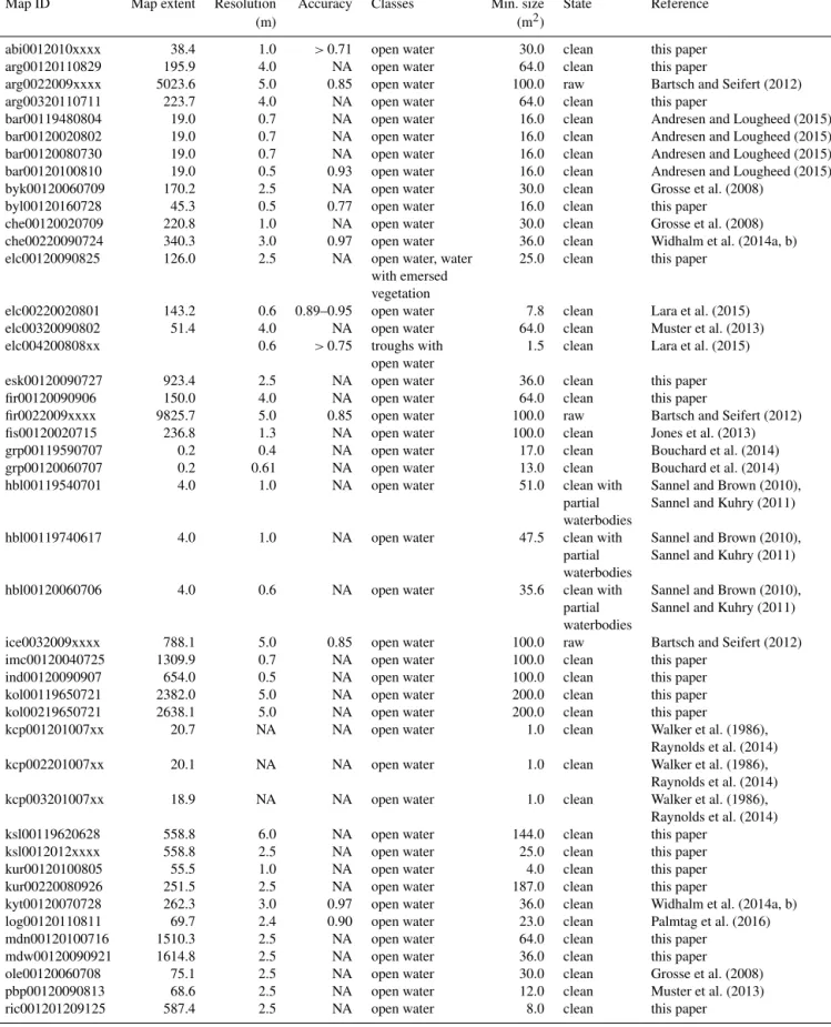
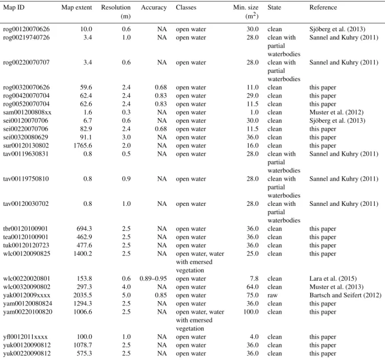
Table 1.Characteristics of waterbody maps. A “clean” map state indicates that the map only includes ponds or lakes. A “raw” map state indi-cates that no manual editing was conducted and that the map may contain rivers, streams, partial waterbodies, or cloud shadows. References indicate whether the map has already been published or was produced specifically for PeRL.

Map ID Map extent Resolution Accuracy Classes Min. size State Reference

(m) (m2)

abi0012010xxxx 38.4 1.0 >0.71 open water 30.0 clean this paper

arg00120110829 195.9 4.0 NA open water 64.0 clean this paper

arg0022009xxxx 5023.6 5.0 0.85 open water 100.0 raw Bartsch and Seifert (2012)

arg00320110711 223.7 4.0 NA open water 64.0 clean this paper

bar00119480804 19.0 0.7 NA open water 16.0 clean Andresen and Lougheed (2015)

bar00120100810 19.0 0.5 0.93 open water 16.0 clean Andresen and Lougheed (2015)

byk00120060709 170.2 2.5 NA open water 30.0 clean Grosse et al. (2008)

byl00120160728 45.3 0.5 0.77 open water 16.0 clean this paper

che00120020709 220.8 1.0 NA open water 30.0 clean Grosse et al. (2008)

che00220090724 340.3 3.0 0.97 open water 36.0 clean Widhalm et al. (2014a, b)

elc00120090825 126.0 2.5 NA open water, water 25.0 clean this paper

with emersed vegetation

elc00220020801 143.2 0.6 0.89–0.95 open water 7.8 clean Lara et al. (2015)

elc00320090802 51.4 4.0 NA open water 64.0 clean Muster et al. (2013)

elc004200808xx 0.6 >0.75 troughs with 1.5 clean Lara et al. (2015)

open water

esk00120090727 923.4 2.5 NA open water 36.0 clean this paper

fir00120090906 150.0 4.0 NA open water 64.0 clean this paper

fir0022009xxxx 9825.7 5.0 0.85 open water 100.0 raw Bartsch and Seifert (2012)

fis00120020715 236.8 1.3 NA open water 100.0 clean Jones et al. (2013)

grp00119590707 0.2 0.4 NA open water 17.0 clean Bouchard et al. (2014)

grp00120060707 0.2 0.61 NA open water 13.0 clean Bouchard et al. (2014)

hbl00119540701 4.0 1.0 NA open water 51.0 clean with Sannel and Brown (2010),

partial Sannel and Kuhry (2011) waterbodies

ice0032009xxxx 788.1 5.0 0.85 open water 100.0 raw Bartsch and Seifert (2012)

imc00120040725 1309.9 0.7 NA open water 100.0 clean this paper

ind00120090907 654.0 0.5 NA open water 100.0 clean this paper

kol00119650721 2382.0 5.0 NA open water 200.0 clean this paper

kol00219650721 2638.1 5.0 NA open water 200.0 clean this paper

kcp001201007xx 20.7 NA NA open water 1.0 clean Walker et al. (1986),

Raynolds et al. (2014)

ksl00119620628 558.8 6.0 NA open water 144.0 clean this paper

ksl0012012xxxx 558.8 2.5 NA open water 25.0 clean this paper

kur00120100805 55.5 1.0 NA open water 4.0 clean this paper

kur00220080926 251.5 2.5 NA open water 187.0 clean this paper

kyt00120070728 262.3 3.0 0.97 open water 36.0 clean Widhalm et al. (2014a, b)

log00120110811 69.7 2.4 0.90 open water 23.0 clean Palmtag et al. (2016)

mdn00120100716 1510.3 2.5 NA open water 64.0 clean this paper

mdw00120090921 1614.8 2.5 NA open water 36.0 clean this paper

ole00120060708 75.1 2.5 NA open water 30.0 clean Grosse et al. (2008)

pbp00120090813 68.6 2.5 NA open water 12.0 clean Muster et al. (2013)

(7)

Table 1.Continued.

Map ID Map extent Resolution Accuracy Classes Min. size State Reference

(m) (m2)

rog00120070626 10.0 0.6 NA open water 30.0 clean Sjöberg et al. (2013)

rog00219740726 3.4 1.0 NA open water 28.0 clean with Sannel and Kuhry (2011)

partial waterbodies

rog00220070707 3.4 0.6 NA open water 28.0 clean with Sannel and Kuhry (2011)

partial waterbodies

rog00320070626 59.6 2.4 0.68 open water 11.0 clean this paper

sam001200808xx 1.6 0.3 NA open water 1.0 clean Muster et al. (2012)

sei00120070706 6.7 0.6 NA open water 30.0 clean Sjöberg et al. (2013)

sei00220070706 82.9 2.4 0.68 open water 11.5 clean this paper

sei00320080629 91.1 3.0 NA open water 36.0 clean this paper

sur00120130802 1765.6 2.0 NA open water 16.0 clean this paper

tav00119630831 0.8 0.5 NA open water 28.0 clean with Sannel and Kuhry (2011)

partial waterbodies

tbr00120100901 694.3 2.5 NA open water 36.0 clean this paper

tea00120100901 462.9 2.5 NA open water 36.0 clean this paper

tuk00120120723 477.6 2.5 NA open water 36.0 clean this paper

wlc00120090825 1400.2 2.5 NA open water, water 25.0 clean this paper

wlc00220020801 153.8 0.6 0.89–0.95 open water 7.8 clean Lara et al. (2015)

wlc00320090802 297.3 4.0 NA open water 64.0 clean Muster et al. (2013)

yak0012009xxxx 2035.5 5.0 0.85 open water 75.0 raw Bartsch and Seifert (2012)

yam00120080824 1294.3 2.5 NA open water 36.0 clean this paper

yam00220100820 1006.6 2.5 NA open water, water 100.0 clean this paper

yfl0012011xxxx 100.0 1.0 NA open water 4.0 clean this paper

yuk00120090812 1078.7 2.5 NA open water 36.0 clean this paper

yuk00220090812 575.3 2.5 NA open water 36.0 clean this paper

6.2 Circum-Arctic waterbody map 6.2.1 Data set structure

The unified vector file PeRL_perma_land.shp contains the permafrost landscapes and the extrapolated waterbody statis-tics (Table 3). Average statisstatis-tics were calculated for 10 km × 10 km boxes within large maps or when four or more maps were present in the permafrost landscapes. Avage statistics are reported with their relative standard er-ror (RE), i.e., the standard erer-ror expressed as a percent-age. The permafrost landscapes are also provided as sep-arate vector files for each region (alaska_perma_land.shp, canada_perma_land.shp, and russia_perma_land.shp) and

contains the landscape characteristic of each permafrost landscape as individual attributes (Appendix B, Tables B1, B2, and B3). The unified vector file (PeRL_perma_land.shp), and the regional files can be joined using the common PER-MID (Appendix B, Table B4).

6.2.2 Spatial and environmental characteristics

Altogether, we identified 230 different permafrost landscapes in the Russian lowlands, 160 in the Canadian lowlands, and 51 in the lowlands of Alaska. PeRL waterbody maps were lo-cated in 28 different permafrost landscapes (Table 4) which cover a total area of 1.4 × 106km2across the Arctic; thereof

(8)

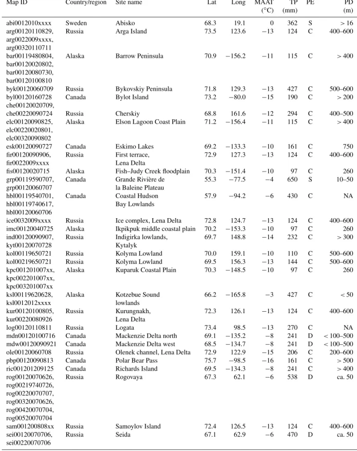
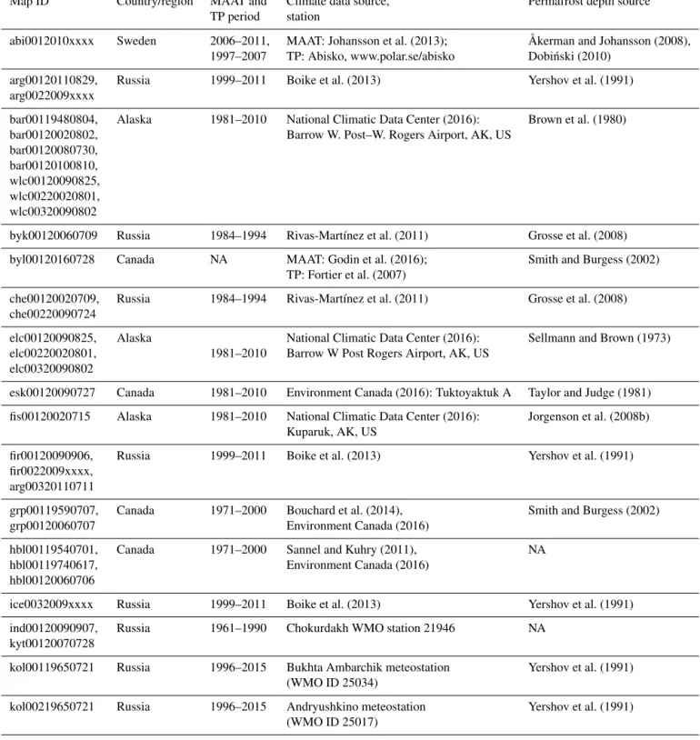
Table 2.Climate and permafrost characteristics for each study area. Latitude (lat) and longitude (long) coordinates are reported in decimal degrees (WGS84). MAAT: mean annual air temperature; TP: total precipitation; PE: permafrost extent (C – continuous, D – discontinuous, S – sporadic); PD: permafrost depth. References to all data sources are listed in Table C1.

Map ID Country/region Site name Lat Long MAAT TP PE PD

(◦C) (mm) (m)

abi0012010xxxx Sweden Abisko 68.3 19.1 0 362 S >16

arg00120110829, Russia Arga Island 73.5 123.6 −13 124 C 400–600

arg0022009xxxx, arg00320110711

bar00119480804, Alaska Barrow Peninsula 70.9 −156.2 −11 115 C >400 bar00120020802,

bar00120080730, bar00120100810

byk00120060709 Russia Bykovskiy Peninsula 71.8 129.3 −13 427 C 500–600

byl00120160728 Canada Bylot Island 73.2 −80.0 −15 190 C >200

che00120020709,

che00220090724 Russia Cherskiy 68.8 161.6 −12 294 C 400–500

elc00120090825, Alaska Elson Lagoon Coast Plain 71.2 −156.4 −11 115 C >400 elc00220020801,

elc00320090802

esk00120090727 Canada Eskimo Lakes 69.2 −133.3 −10 161 C 750

fir00120090906, Russia First terrace, 72.9 127.3 −13 124 C 400–600

fir0022009xxxx Lena Delta

fis00120020715 Alaska Fish–Judy Creek floodplain 70.3 −151.4 −10 97 C 260

grp00119590707, Canada Grande Rivière de 55.3 −77.5 −4 650 S 10–50

grp00120060707 la Baleine Plateau

hbl00119540701, Canada Coastal Hudson 57.9 −94.2 −6 430 C NA

hbl00119740617, Bay Lowlands

hbl00120060706

ice0032009xxxx Russia Ice complex, Lena Delta 72.8 124.7 −13 124 C 400–600 imc00120040725 Alaska Ikpikpuk middle coastal plain 70.2 −153.3 −10 97 C 260 ind00120090907, Russia Indigirka lowlands, 69.7 148.8 −14 232 C >300

kyt00120070728 Kytalyk

kol00119650721 Russia Kolyma Lowland 70.0 159.1 −10 110 C 500–600

kol00219650721 Russia Kolyma Lowland 69.5 156.3 −13 144 C 500–600

kpc001201007xx, Alaska Kuparuk Coastal Plain 70.3 −148.5 −10 97 C 260 kpc002201007xx,

kpc003201007xx

ksl00119620628, Alaska Kotzebue Sound 66.2 −165.8 −3 427 C <50

ksl0012012xxxx lowlands

kur00120100805, Russia Kurungnakh, 72.3 126.1 −13 124 C 400–600

kur00220080926 Lena Delta

log00120110811 Russia Logata 73.4 98.5 −13 270 C NA

mdn00120100716 Canada Mackenzie Delta north 69.1 −135.2 −8 241 D <100–500 mdw00120090921 Canada Mackenzie Delta west 68.5 −134.7 −8 241 D <100–500 ole00120060708 Russia Olenek channel, Lena Delta 72.9 122.9 −15 206 C 200–600

pbp00120090813 Canada Polar Bear Pass 75.7 −98.5 −16 161 C >500

ric001201209125 Canada Richards Island 69.5 −134.3 −8 241 C >400

rog00120070626, Russia Rogovaya 67.3 62.1 −6 538 D ca. 50

rog00219740726, rog00220070707, rog00320070626, rog00420070704, rog00520070704

sam001200808xx Russia Samoylov Island 72.4 126.5 −13 124 C 400–600

sei00120070706, Russia Seida 67.1 62.9 −6 470 D ca. 50

(9)

Table 2.Continued.

Map ID Country/region Site name Lat Long MAAT TP PE PD

(◦C) (mm) (m)

sur00120130802 Russia Surgut 62.3 74.6 −17 400 S 50–300

tav00119630831,

tav00119750810, Sweden Tavvavuoma 68.5 20.9 −3 451 S <25

tav00120030702

tbr00120100901, Canada Tanzin Upland Beaulieu River 62.7 −115.2 −4 289 D NA tea00120100901

tuk00120120723 Canada Tuktoyaktuk Peninsula 69.9 −130.4 −10 161 C 750 wlc00120090825, Alaska Wainwright lower coastal plain 70.9 −156.2 −11 115 C >400 wlc00220020801,

wlc00320090802

yak0012009xxxx Russia Yakutsk 62.1 130.3 −10 228 C 200–300

yam00120080824, Russia Yamal Peninsula 71.5 70.0 −6 260–400 C 100–500

yam00220100820

yfl0012011xxxx Alaska Yukon Flats basin 66.2 −145.9 −5 309 D 90

yuk00120090812, Alaska Yukon–Kuskokwim Delta 60.9 −162.4 61 471 C 100–200 yuk00220090812

1.0 × 106km2 are in Russia, 2.1 × 105km2 in Canada, and 1.7×105km2in Alaska. About 65 % of the extrapolated area was classified as high confidence (Fig. 3). The highest land-scape average areal fraction of water surface was 21 % (Fig. 4 and Table 3), and there was a waterbody density per square kilometer of 57 (Fig. 5 and Table 4).

RE of areal fraction for different subsets or maps within a permafrost landscape was about 7 % on average, with a maximum of 30 % (Table 4). RE for waterbody density was 8 % on average, with a maximum of 50 %. Our extrapolated area (1.4 × 106km2) represents 17.0 % of the current Arc-tic permafrost lowland area (below 300 m a.s.l.). PeRL pro-vides pond and lake estimates for about 29 % (in area) of the Alaskan lowlands, 7 % of the Canadian lowlands, and 21 % of the Russian lowlands. Together all extrapolated land-scapes contributed about 7 % to the current estimated Arc-tic permafrost area (Brown et al., 1998). In Alaska, wa-terbody maps were missing for permafrost landscapes with isolated permafrost (16 % of total area) or rocky lithology (36 % of total area). Dominant types of surficial geology that were not mapped include colluvial sites and sites with bedrock or of glacial origin, which together contribute 61 % to the total area. In Canada, neither isolated nor sporadic permafrost were inventoried (22 % of total area) nor was this done for areas with a ground ice content of 10–20 % or less (23 % of total area). Six of the nineteen geology classes were inventoried, which contributes 75 % to the total area. Six of seven lithology types with an areal coverage of 90 % were represented. In Russia, waterbody maps were not avail-able in the discontinuous permafrost zone (13 % of the to-tal area). No maps were present in regions with the geolo-gical type “deluvial–coluvial and creep” which accounts for 28 % of the total area.

Figure 3.Confidence for permafrost lowland landscapes. Confi-dence class 1 (high confiConfi-dence) designates permafrost landscapes where waterbody maps are available in lowland areas. Confidence class 2 (low confidence) represents permafrost landscapes with ex-trapolated waterbody statistics. No-value (dark grey) areas indicate that no maps were available in these permafrost landscapes. Light-grey areas indicate terrain with elevations (GTOPO 30, USGS) higher than 300 m a.s.l. which were not considered in the extrapola-tion. Permafrost boundary was derived from the regional databases.

7 Discussion

7.1 Classification accuracy and variability

The accuracy of the individual waterbody map depends on the spectral and spatial properties of the remote-sensing im-agery employed for classification as well as the

(10)

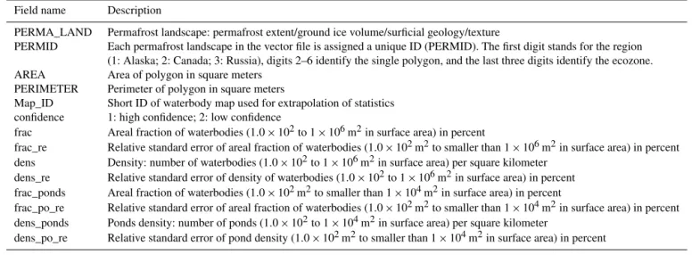
classifica-Table 3.Attributes of ESRI shape file PeRL_perma_land.shp.

Field name Description

PERMA_LAND Permafrost landscape: permafrost extent/ground ice volume/surficial geology/texture

PERMID Each permafrost landscape in the vector file is assigned a unique ID (PERMID). The first digit stands for the region (1: Alaska; 2: Canada; 3: Russia), digits 2–6 identify the single polygon, and the last three digits identify the ecozone. AREA Area of polygon in square meters

PERIMETER Perimeter of polygon in square meters

Map_ID Short ID of waterbody map used for extrapolation of statistics confidence 1: high confidence; 2: low confidence

frac Areal fraction of waterbodies (1.0 × 102to 1 × 106m2in surface area) in percent

frac_re Relative standard error of areal fraction of waterbodies (1.0 × 102m2to smaller than 1 × 106m2in surface area) in percent dens Density: number of waterbodies (1.0 × 102to 1 × 106m2in surface area) per square kilometer

dens_re Relative standard error of density of waterbodies (1.0 × 102to 1 × 106m2in surface area) in percent frac_ponds Areal fraction of waterbodies (1.0 × 102m2to smaller than 1 × 104m2in surface area) in percent

frac_po_re Relative standard error of areal fraction of waterbodies (1.0 × 102m2to smaller than 1 × 104m2in surface area) in percent dens_ponds Ponds density: number of ponds (1.0 × 102to 1 × 104m2in surface area) per square kilometer

dens_po_re Relative standard error of pond density (1.0 × 102m2to smaller than 1 × 104m2in surface area) in percent

Figure 4.Areal fraction of waterbodies with surface areas between 1.0 × 102and 1.0 × 106m2. Permafrost boundary was derived from the regional databases.

tion method. In general, open-water surfaces show a high contrast to the surrounding land area in all utilized spec-tral bands, i.e., panchromatic, near-infrared, and X-band, since water absorbs most of the incoming radiation (Grosse et al., 2005; Muster et al., 2013). Ground surveys of wa-terbody surface area were available for only a few study sites. Accuracy ranged between 89 % for object-oriented mapping of multispectral imagery (Lara et al., 2015), 93 % for object-oriented mapping of panchromatic imagery (An-dresen and Lougheed, 2015), and more than 95 % for a su-pervised maximum-likelihood classification of multispectral aerial images (Muster et al., 2012). Errors in the classifica-tion may be largely due to commission errors: i.e., the spec-tral signal is misinterpreted as water where in reality it may

Figure 5.Waterbody density per square kilometer for waterbodies with surface areas of between 1.0 × 102 and 1.0 × 106m2within permafrost landscape units. Permafrost boundary was derived from the regional databases.

be land surface. Many shallow ponds and pond–lake mar-gins are characterized by vegetation growing or floating in the water which cannot be adequately classified from single-band imagery (Sannel and Brown, 2010). PeRL classifica-tions dating from early August are likely most affected since the abundance of aquatic plants peaks around that time of year. In some cases, even multispectral imagery cannot dis-tinguish between lake and land because floating vegetation mats fully underlain by lake water may spectrally appear like a land surface (Parsekian et al., 2011).

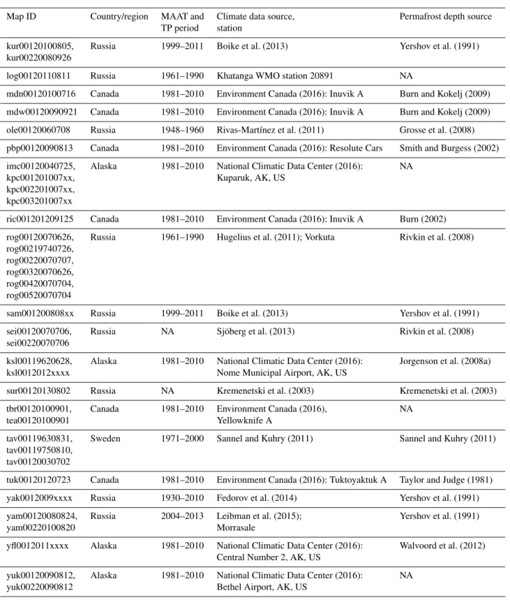
Seasonal processes, such as snowmelt, progressing thaw depth, evaporation, and precipitation do affect the extent of surface water. Waterbody maps therefore reflect the local

(11)

wa-T ab le 4. Extrapolated w aterbody statistics for permafrost landscapes. Permafrost extent (PE) is reported as follo ws: C – continuous; D – discontinuous; and S – sporadic. Extrapolated statistics include areal fraction and w aterbody number per square ki lometer for w aterbodies ( ≥ 1 .0 × 10 2and ≤ 1 .0 × 10 6m 2) and ponds ( ≥ 1 .0 × 10 2and < 1 .0 × 10 4m 2). Numbers in brack ets denote the relati v e error in percent. The RE w as calcul ated for 10 km × 10 km box es within lar ge maps or when four or more small maps could be av eraged. The RE is the standard error expressed as a percentage. The standard error is the standard de viation of the sampling distrib ution of a stat istic. Country/re gion Ecozone PE Ground ice Surficial geology Lithology Fraction Density Pond Pond (v ol %) fraction density Arctic tundra C 10–40 alluvial–marine Sandy 7.3 (4.6) 17.6 (3.4) 1.6 (2.8) 16.9 (3.4) Arctic tundra C < 10 eolian, sand Sandy 11.1 (4.9) 21.3 (10.3) 1.8 (11.4) 20.4 (10.4) Arctic tundra C > 40 glaciomarine Silty 8 (N A) 28 (N A) 1.8 (N A) 27.3 (N A) Alaska Bering taig a D > 40 eolian, loess Silty 10.5 (N A) 7.3 (N A) 1.1 (N A) 5.9 (N A) Bering taig a S 10–40 fluvial, abandoned terrace Silty 9.9 (5.3) 6.2 (3.8) 0.7 (3.3) 5.1 (3.9) Bering tundra C > 40 eolian, loess Silty 5.7 (11.8) 1.6 (18) 0.3 (13.7) 1.1 (28.5) Intermontane boreal D 10–40 fluvial, abandoned terrace Silty 7.1 (N A) 2.9 (N A) 0.3 (N A) 2.4 (N A) Canada Northern Arctic C < 20 colluvial fines Sandy Loam 15.1 (N A) 42.9 (N A) 5.9 (N A) 40.6 (N A) Northern Arctic C < 10 till v eneer N A 3.7 (N A) 57 (N A) 2.1 (N A) 50.7 (N A) Southern Arctic C > 20 glaciofluvial plain Or g anic 7.6 (4.5) 5.7 (3.4) 0.5 (3) 5.3 (3.4) Southern Arctic C > 20 till blank et Clay 13.2 (3.8) 1.9 (3.2) 0.2 (5.3) 1.0 (5.0) Southern Arctic D < 20 alluvial deposits Loam 7.7 (6.2) 6.9 (5.3) 0.8 (5.2) 6.2 (5.4) T aig a plain D < 20 alluvial deposits Loam 21.1 (1.4) 7.6 (1.7) 1.1 (1.8) 5.4 (2.4) T aig a Shield D < 20 till v eneer Sand 8 (13.9) 7.0 (1.9) 1.0 (1.7) 5.8 (1.2) T aig a Shield D < 20 undi vided Sand 10.8 (3.0) 2.7 (2.1) 0.3 (3.4) 1.7 (3.0) East Siberian taig a C > 40 alluvial–limnetic Coarse 5.3 (10.1) 1 (8.8) 0 (11.5) 0.7 (9.6) East Siberian taig a C > 40 alluvial–limnetic Medium 4.9 (3.8) 2.5 (4.2) 0.4 (4.7) 2.0 (5.0) Northeast Siberian coastal tundra C > 40 alluvial–limnetic Medium 8.3 (N A) 18.2 (N A) 0.8 (N A) 17.6 (N A) Northeast Siberian taig a C > 40 alluvial–limnetic Or g anic 16.7 (10.2) 3.5 (6.3) 0.4 (5.7) 2.3 (6.4) Northeast Siberian taig a C > 40 alluvial–limnetic Coarse 5.3 (10.1) 1 (8.8) 0 (11.5) 0.7 (9.6) Northeast Siberian taig a C > 40 co v er , loess lik e deposits, Medium 1.1 (N A) 3.3 (N A) 0.2 (N A) 3.1 (N A) loess and clays Russia Northwest Russian No v aya Zemlya tundra C < 20 glacial Medium 6.3 (28.1) 12.7 (21.4) 1.4 (24.6) 11.5 (21.5) T aimyr –Central Siberian tundra C > 40 alluvial–limnetic Or g anic 10.3 (10.5) 38.8 (50.1) 2.1 (27.5) 37.8 (51.3) T aimyr –Central Siberian tundra C 20–40 alluvial–limnetic Or g anic 7.2 (N A) 23.8 (N A) 2.5 (N A) 23.1 (N A) T aimyr –Central Siberian tundra C 20–40 glacial Medium 3.6 (N A) 4.5 (N A) 0.4 (N A) 4.1 (N A) W est Siberian taig a S 20–40 or g anic deposits Or g anic 16.7 (2.2) 20.2 (2.1) 3 (2.4) 17.6 (2.2) Y amal–Gydan tundra C > 40 marine Medium 8.9 (5.0) 3.6 (3.1) 0.4 (2.9) 2.7 (3.2) Y amal–Gydan tundra C 20–40 marine Banded 6.1 (2.3) 8.6 (2.7) 0.8 (2.7) 7.8 (2.7)

(12)

ter balance at the time of image acquisition. Seasonal reduc-tion in surface water extent, however, is largest in the first 2 weeks following snowmelt (Bowling et al., 2003). All PeRL maps date from the late summer season so that snowmelt and the early summer season are excluded. Changes of water ex-tent in late summer are primarily due to evaporation and pre-cipitation. In a study area on the Barrow Peninsula, Alaska, we find that the open-water extent varies between 6 and 8 % between the beginning and end of August of different years. However, the effect is hard to quantify as other factors such as spectral properties and resolution also impact classifica-tions of different times at the same site. Seasonal variaclassifica-tions may be larger in the case of heavy rain events right before image acquisition but ultimately depend on local conditions which control surface and subsurface runoff.

7.2 Uncertainty of circum-Arctic map

Uncertainties regarding the extrapolation of waterbody dis-tributions arise from (i) the combination of different water-body maps, (ii) the accuracy of the underlying regional per-mafrost maps, and (iii) the level of generalization inherent in the permafrost landscape units.

Waterbody statistics of permafrost landscapes are derived from diverse remote-sensing imagery. Imagery dates from different years and months and features different image prop-erties. However, the effect of seasonal variability or image properties on the average statistic is small compared to the natural variability within and between permafrost landscape units.

Permafrost landscapes present a unified circum-Arctic cat-egorization to upscale waterbody distributions. Due to the uncertainty and scale of the regional PLM, however, it can-not be expected that nonoverlapping waterbody maps within the same permafrost landscape have the same size distribu-tion. The regional PLM are themselves extrapolated prod-ucts where finite point sources of information have been used to describe larger spatial domains. No error or uncertainty measure, however, was reported for the regional maps. In ad-dition, the variables used to describe permafrost landscapes present the dominant classes within the landscape unit. Thus, certain waterbody maps may represent landscape subtypes that are not represented by the reported average statistic. For example, two permafrost landscapes have been classified in the Lena Delta in northern Siberia. The southern and east-ern parts of the delta are characterized by continuous per-mafrost with ground ice volumes larger than 40 %, alluvial– limnetic deposits, and organic substrate. Local studies entiate this region further based on geomorphological differ-ences and ground ice content. The yedoma ice complex in the southern part features a much higher ground ice content of up to 80 % and higher elevations than the eastern part; this is, however, not resolved in the Russian PLM. These subre-gional landscape variations are also reflected in the water-body size distributions which are significantly different for

the southern and eastern part of the delta. In the averaged statistics this is indicated by a high relative error of 11 and 28 % for the areal fraction of waterbodies and ponds, respec-tively, and of about 50 % for waterbody density estimates. In this case, the permafrost landscape unit in that area does not adequately reflect the known distribution of ground ice and geomorphology and demonstrates the need to further im-prove PLM in the future.

7.3 Potential use of database and future development Waterbody maps and distribution statistics are the most ac-curate at site level. On this scale, maps can be used as a base-line to detect changes in surface inundation for seasonal, in-terannual, and decadal periods. Site-level size distributions can also be used to validate statistical extrapolation methods which have previously been used to extrapolate from coarser databases to finer scales (Downing et al., 2006; Seekell et al., 2010). Validation of these approaches has questioned the validity of power laws for smaller lakes and ponds but has also been limited to waterbodies as small as 1.0 × 104m2, i.e., 2 orders of magnitude larger than the minimum size in PeRL data sets.

The circum-Arctic map provides spatially extrapolated in-formation for larger-scale applications. Coarse-scale global databases such as the Global Lakes and Wetlands database (GLWD) by Lehner and Döll (2004) are used in global Earth system models to represent the water fraction in model grid cells (Wania et al., 2013). The GLWD renders a reliable in-ventory of lakes larger 1 km2(Lehner and Döll, 2004). Com-pared to the GLWD, PeRL inventoried up to 21 % additional waterbody area. Moreover, ponds are the most frequent wa-terbody type (45–99 %). In light of the observed scaling of biogeochemical processes with waterbody surface area (Wik et al., 2016), PeRL results emphasize the need to include wa-terbodies of 1.0 × 106m2 and smaller in conjunction with their size distributions in physical and biogeochemical mod-els of the high-latitude surface. Moreover, the combination of waterbody size distributions with landscape properties can motivate further study for process-based predictive simula-tions both on the site and regional scale. However, users should be aware of the map’s uncertainty when using it to upscale landscape properties such as methane or heat fluxes. For this purpose, users should refer to the reported spatial variability, confidence class, and extensive metadata.

PeRL’s permafrost landscape units represent the least com-mon denominator across the Arctic where landscape proper-ties have been strongly generalized. More detailed informa-tion about landscape properties was available for the Cana-dian database and northern Alaska (Jorgensen et al., 2014) but not for central and southern Alaska or Russia. We sug-gest that more detailed and accurate classes of ground ice as well as further refinement of physiography within the broad lowland zone will likely explain differences in waterbody distributions between different maps in the same permafrost

(13)

landscape. Regionally different methodologies currently pro-hibit a comparison of permafrost landscapes between regions and extrapolation across regions. The harmonization of land-scape properties, delineation of common terrain units, and extrapolation methods for the whole Arctic require a coordi-nated circum-Arctic effort.

Our extrapolated area (1.4 × 106km2) represents only 7.0 % of the current estimated Arctic permafrost area (Brown et al., 1998) but about 17 % of the current Arctic permafrost lowland area (below 300 m a.s.l.) where most of the Arctic lakes are located (Lehner and Döll, 2004; Smith et al., 2007; Grosse et al., 2013). With a few exceptions, the reported sites are predominantly located in coastal areas. In particu-lar, the lake-rich permafrost lowlands of Canada and central Siberia are underrepresented, despite their large spatial cov-erage. Underrepresented landscape types are areas with dis-continuous, isolated, or sporadic permafrost, as well as ar-eas in boreal regions. PeRL maps are conservative estimates of surface inundation as most maps capture open water only and do not include ponds smaller than 1.0 × 102m2in size. PeRL maps with resolutions of less than 1 m, however, indi-cate the presence of many waterbodies smaller than the cur-rent threshold of 1.0 × 102m2. These very small waterbod-ies as well as water areas with emersed vegetation are highly productive environments that require attention in future map-ping efforts.

8 Data availability

Waterbody maps, study area boundaries, and maps of re-gional permafrost landscapes including a link to detailed metadata are available at https://doi.pangaea.de/10.1594/ PANGAEA.868349 (Muster et al., 2017).

9 Conclusions

PeRL maps and statistics provide a great resource for a large suite of applications across the Arctic such as resource and habitat management, hydrological and ecological modeling, pond and lake change detection, and upscaling of biogeo-chemical processes. PeRL maps includes waterbodies with surface areas as small as 1.0 × 102m2; this complements available global databases and increases waterbody size res-olution by 2–4 orders of magnitude. Ponds, i.e., waterbodies with surface areas smaller than 1.0 × 104m2are the domi-nant waterbody type found in all study areas across the Arc-tic. This demonstrates the need to include small waterbod-ies and parameterize size distributions in global land surface models. Furthermore, PeRL presents a baseline that allows future studies to investigate the direction and magnitude of past and future Arctic surface inundation. The current compi-lation of high-resolution waterbody maps underlines the need to produce more: vast areas in all regions are still unmapped regarding small waterbodies, especially the Canadian low-lands and boreal regions of Russia. Future mapping efforts should therefore focus equally on filling gaps and monitor-ing inventoried sites. The combination of waterbody statistics and landscape properties has great potential to improve our understanding of environmental drivers of surface inunda-tion in permafrost lowlands. However, permafrost landscape maps need to be improved by increasing the level of detail as well by harmonizing mapping and extrapolation approaches across Arctic regions.

(14)

Appendix A: Image processing and subgrid sampling

A1 Processing of TerraSAR-X imagery

Geocoded EEC products obtained from the German Space Agency (DLR) are delivered in radar brightness. They are projected to the best available digital elevation model (DEM), i.e., Shuttle Radar Topography Mission (SRTM) X-band DEMs (30 m resolution) and SRTM C-X-band DEMs (90 m resolution). For the remaining areas, the 1 km reso-lution Global Land One-kilometer Base Elevation Project (GLOBE) DEM is used. The EEC is a detected multi-look product with reduced speckle and approximately square cells on the ground. The slant-range resolution of the image is 1.2 m, which corresponds to 3.3–3.5 m projected on the ground for incidence angles between 45 and 20◦and an az-imuth resolution of 3.3 m (Eineder et al., 2008). SSC were geocoded to the Data User Element(DUE) Permafrost DEM, and no multi-looking was applied.

A2 Subgrid sampling

In large study areas we performed a subgrid analysis, i.e., we selected waterbodies within equally sized boxes and av-eraged statistics from all boxes of the study area. In order to determine a representative box size, we compared the vari-ability of waterbody distribution statistics within three study areas in Russia, Canada, and Alaska. In each study area, we selected waterbodies from a minimum of 5 and up to 50 ran-domly distributed boxes with varying sizes of 5 km × 5 km, 10 km × 10 km, and 20 km × 20 km. We calculated the stan-dard error (SE) of the mean of all statistics across all boxes of the same size. SE of density (waterbody number per square kilometer) and waterbody mean surface area was lowest for 10 km × 10 km boxes. SE increased for 20 km × 20 km boxes, which is probably due to the significantly lower number of boxes that could be sampled. Only 12 PeRL sites have a study area larger than 1000 km2that would allow sampling a min-imum of five boxes of 20 km × 20 km in size. A box size of 10 km×10 km allows the subsampling of 26 sites with a mini-mum of five boxes. Taking into account the overall variability of distributions and the possible number of subgrid samples, a box size of 10 km × 10 km was chosen for subgrid analysis. Subgrid analysis was conducted for study areas larger than 300 km2.

(15)

T ab le A1. Metadata about image processing and classification. PREP: preprocessing steps; bands used for classification with their corresponding spectral range; POP: post-processing steps (ME: manual editing, includes remo v al of ri v ers, streams, partial lak es, shado ws, streets and g ap-filling). Map ID Imagery Softw are PREP Band(s) Spectral range Method POP Reference abi0012010xxxx orthophoto GD AL, SA GA GIS, 1. image se gmentation using orthophoto red (1 m) + 610–680 nm se gmentation ME this paper (Lantmäteriet, Orfeo toolbox RGB (1 m) and DEM (2 m), slope (2 m) → SVM I2014/00691); minimum object size 130 m 2 SPO T -5; DEM 2. classification of w at ermask: SVM classifier using red band and slopes ar g00120110829 K OMPSA T -2 ENVI 4.8, georeferencing NIR 760–900 nm density slice ME this paper ArcGIS 12 ar g0022009xxxx, RapidEye N A georeferencing, histogram B, G, blue: 440–510 nm, object-oriented N A Bartsch and Seifert (2012) fir0022009xxxx, matching routine for R, RE, green: 520–590 nm, classification ice0032009xxxx radiometric normalization, NIR red: 630–685 nm, mosaicking RE: 690–730 nm, NIR: 760–850 nm ar g00320110711 K OMPSA T -2 ENVI 4.8, georeferencing NIR 760–900 nm density slice ME this paper ArcGIS 10 bar00119480804 aerial imagery ENVI 4.4 co-re gistration and orthorectification P AN N A object-oriented ME Andresen and Lougheed (2015) using an image-to-image correction classification (RMSE of 1.0 m) bar00120020802 Quickbird ENVI 4.4 co-re gistration and orthorectification P AN 445–900 nm object-oriented ME Andresen and Lougheed (2015) using an image-to-image correction classification (RMSE of 1.0 m) bar00120080730 Quickbird ENVI 4.4 co-re gistration and orthorectification P AN 445–900 nm object-oriented ME Andresen and Lougheed (2015) using an image-to-image correction classification (RMSE of 1.0 m) bar00120100810 W orldV ie w-2 ENVI 4.4 co-re gistration and orthorectification P AN 450–800 nm object-oriented ME Andresen and Lougheed (2015) using an image-to-image correction classification (RMSE of 1.0 m) byk00120060709 SPO T -5 ArcGIS georeferenced to topographic P AN 480–710 nm density slice ME Lara et al. (2015) maps of scale 1 :100 000 byl00120160728 Pleiades-1B Geomatica 2015, pan-sharpening, B, G, 430–550, 490–610, unsupervised ME this paper ArcGIS 10.4 orthorectification R, NIR 600–720, 750–920 nm k-means classification che00120020709 IK ONOS-2 ArcGIS orthorectification P AN 760–850 nm density slice ME Grosse et al. (2008) che00220090724 ALOS PRISM N A N A P AN 520–770 nm density slice ME W idhalm et al. (2014a, b) elc00120090825, T erraSAR-X ENVI 4.4 g amma filter (11 × 11 pix el) X w av elength 31 mm, unsupervised ME this paper wlc00120090825 frequenc y 9.6 GHz k-means classification elc00220020801, Quickbird ArcGIS 10.2, principle component analysis R, B, 450–520, 560–600, object-oriented ME Lara et al. (2015) wlc00220020801 eCognition 9.1 on raster bands, pan-sharpening G, IR 630–690, 760–890 nm classification elc00320090802, K OMPSA T -2 ENVI 4.8, georeferencing NIR 760–900 nm density slice ME Muster et al. (2013) wlc00320090802 ArcGIS 10

(16)

T ab le A1. Continued. Map ID Imagery Softw are PREP Band(s) Spectral range Method POP Reference elc004200808xx Quickbird ArcGIS 10.2, principle component analysis R, B, 450–520, 560–600, object-oriented N A Lara et al. (2015) eCognition 9.2 on raster bands, pan-sharpening G, IR 630–690, 760–890 nm classification esk00120090727 T erraSAR-X ENVI 4.8, ArcGIS 10 lee filter (3 × 3 pix el), X w av elength 31 mm, unsupervised ME this paper g amma filter (11 × 11 pix el) frequenc y 9.6 GHz k -means classification fir00120090906 K OMPSA T -2 ENVI 4.8, ArcGIS 10 georeferencing NIR 760–900 nm density slice ME this paper fis00120020715 airborne ENVI 4.5 N A P AN bandwidth of 135 density slice ME Jones et al. (2013) orthorectified or 270 MHz radar imagery (IFSAR) grp00119590707 aerial imagery ArcGIS 10.0 scanning (1814 dpi ), black and N A manual N A Bouchard et al. (2014) georeferencing white (RMSE = 1.8 m (4.2 pix)) grp00120060707 QuickBird ArcGIS 10.0 geometric correction (cubic P AN 450–900 nm manual N A Bouchard et al. (2014) con v olution resampling) hbl00119540701 aerial imagery ENVI 4.5, resampling of pix el resolution P AN N A manual delineation N A Sannel and Bro wn (2010), ENVI 4.7, to 0.6 m, georeferenced Sannel and K uhry (2011) ArcGIS 9 to QuickBird image from 2006 RMSE of 0.38–1.42 hbl00119740617 aerial imagery ENVI 4.5, resampling of pix el resolution P AN N A manual delineation N A Sannel and Bro wn (2010), ENVI 4.7, to 0.6 m, georeferenced Sannel and K uhry (2011) ArcGIS 9 to QuickBird image from 2006 RMSE of 0.38–1.42 hbl00120060706 QuickBird ENVI 4.5, N A P AN 405–1053 nm manual delineation N A Sannel and Bro wn (2010), ENVI 4.7, Sannel and K uhry (2011) ArcGIS 9 imc00120040725 QuickBird-2 ENVI 5.0, orthorectification P AN 760–850 nm density slice ME this paper ArcGIS 10.3 ind00120090907 W orldV ie w-1 ENVI 5.0, orthorectification P AN 400–900 nm density slice, ME this paper ArcGIS 10.3 opening filter 3 × 3 k ol00119650721, COR ON A ArcGIS 9 georeferencing P AN N A manual delineation N A this paper k ol00219650721 kpc001201007xx, digital true N A N A R, G, N A manual delineation N A W alk er et al. (1986), kpc002201007xx, color aerial B Raynolds et al. (2014) kpc003201007xx imagery ksl00119620628 Corona KH4 ENVI 4.8, ArcGIS 10 georeferencing to P AN N A density slice ME this paper Landsat ETM & TM (RMSE = 10 m) ksl0012012xxxx SPO T -5 eCognition 8 principal component G, R, N A object-oriented ME this paper analysis on visible NIR cla ssification and IR bands

(17)

T ab le A1. Continued. Map ID Imagery Softw are PREP Band(s) Spectral range Method POP Reference kur00120100805 Geoe ye ENVI 4.8, pan-sharpening, NIR 760–900 nm unsupervised ME this paper ArcGIS 10 orthorectification k-means (RMSE: 0.36 m) cla ssification kur00220080926 ALOS PRISM PCI Geomatica, orthorectification based P AN 520–770 nm manual delineation M E this paper ArcGIS 9 on o wn stereo DEM k yt00120070728 ALOS PRISM ENVI 4.8, orthorectification based P AN 520–770 nm density slice M E W idhalm et al. (2014a, b) ArcGIS 10 on o wn stereo DEM log00120110811 QuickBird ENVI 5.1 N A NIR, R, 485-830 nm supervised ME P almtag et al. (2016) G, B maximum-lik elihood classification mdn00120090921 T erraSAR-X ENVI 4.8, lee filter (3 × 3 pix el), X w av elength 31 mm, density slice; ME this paper ArcGIS 10 g amma filter (11 × 11 pix el) frequenc y 9.6 GHz mdn00120100716 T erraSAR-X ENVI 4.8, lee filter (3 × 3 pix el), X w av elength 31 mm, k-means classification: ME this paper ArcGIS 10 g amma filter (11 × 11 pix el) frequenc y 9.6 GHz 15 classes, fi v e iterations; classes 1–3 identified as w ater ole00120060708 SPO T -5 ArcGIS georeferenced to topographic P AN 480–710 nm density slice ME Grosse et al. (2008) maps of scale 1 :100 000 pbp00120090813 T erraSAR-X ENVI 4.8, g amma filter (11 × 11 pix el) X w av elength 31 mm, density slice majority filter Muster et al. (2013) ArcGIS 10 frequenc y 9.6 GHz (7 × 7 pix el) to reduce spurious pix els in classification, ME ric001201209125 T erraSAR-X ENVI 4.8, lee filter (3 × 3 pix el), X w av elength 31 mm, k-means classification: ME this paper ArcGIS 10 g amma filter (11 × 11 pix el) frequenc y 9.6 GHz 15 classes, fi v e iterations; classes 2–4 were identified as w ater rog00120070626 QuickBird ArcGIS N A P AN 760–850 nm manual delineation N A Sjöber g et al. (2013) rog00219740726 aerial imagery ENVI 4.5, resampling of pix el P AN N A manual delineation N A Sannel and K uhry (2011) ENVI 4.7, resolution to 0.6 m, ArcGIS 9 georeferenced to QuickBird image from 2007 with RMSE of 0.20–1.25, rog00220070707 QuickBird ENVI 4.5, N A P AN 760–850 nm manual delineation N A Sannel and K uhry (2011) ENVI 4.7, ArcGIS 9 rog00320070626 QuickBird-2 classificat ion in re-georeferenced B, G, blue: 450–520 nm, supervised; see more in M E this paper Definiens using field R, NIR green: 520-600 nm, INFO_Qbird_classification_ Professional 5.0, measured red: 630–690 nm, v ersion4.pdf post-processing GPS points NIR: 760–890 nm with ArcGIS

(18)

T ab le A1. Continued. Map ID Imagery Softw are PREP Band(s) Spectral range Method POP Reference rog00420070704 QuickBird-2 classi fication in re-georeferenced B, G, blue: 450–520 nm, supervised; see more in ME this paper Definiens using field R, NIR green: 520–600 nm, INFO_Qbird_classification_ Professional 5.0, measured red: 630–690 nm, v ersion4.pd post-processing GPS points NIR: 760–890 nm with ArcGIS rog00520070704 QuickBird-2 classi fication in re-georeferenced B, G, 450–520, supervised; see more in ME this paper Definiens using field R, NIR 520–600, INFO_Qbird_classification_ Professional 5.0, measured 630–690, v ersion4.pdf post-processing GPS points 760–890 nm with ArcGIS sam001200808xx aerial imagery ENVI 4.8, georeferencing NIR N A N A ME Muster et al. (2012) ArcGIS 10 sei00120070706 QuickBird ArcGIS N A P AN 450–900 nm manual delineation N A Sjöber g et al. (2013) sei00220070706 QuickBird-2 classi fication in re-georeferenced B, G, blue: 450–520 nm, supervised; see more in ME this paper Definiens using field R, green: 520–600 nm, INFO_Qbird_classification_ Professional 5.0, measured NIR red: 630–690 nm, v ersion4.pdf post-processing GPS points NIR: 760–890 nm with ArcGIS sur00120130802 T erraSAR-X ENVI 4.8, orthorectification, X w av elength 31 mm, threshold ME this paper ArcGIS 10 g amma filter 10 × 10 m frequenc y 9.6 GHz classification ta v00119630831 aerial imagery ENVI 4.5, resampling of pix el resolution P AN N A manual delineation N A Sannel and K uhry (2011) ENVI 4.7, to 0.6 m, georeferenced to ArcGIS 9 IK ONOS image from 2003 wihth RMSE of 1.28-3.31 ta v00119750810 aerial imagery ENVI 4.5, resampling of pix el resolution to P AN N A manual delineation N A Sannel and K uhry (2011) ENVI 4.7, 0.6 m, georeferenced ArcGIS 9 to IK ONOS image from 2003 with RMSE of 0.60–2.38 ta v00120030702 IK ONOS ENVI 4.5, resampling of pix el P AN 760–850 nm manual delineation N A Sannel and K uhry (2011) ENVI 4.7, resolution to 0.6 m ArcGIS 9 tbr00120100901, T erraSAR-X ENVI 4.8, lee filter (3 × 3 pix el), X w av elength 31 mm, k -means classification: ME this paper tea00220100901 ArcGIS 10 g amma filter (11 × 11 pix el) frequenc y 9.6 GHz 15 classes, fi v e iterations tuk00120120723 T erraSAR-X ENVI 4.8, lee filter (3 × 3 pix el), X w av elength 31 mm, k -means classification: ME this paper ArcGIS 10 g amma filter (7 × 7 pix el) frequenc y 9.6 GHz 15 classes, fi v e iterations yam00120080824 T erraSAR-X ENVI 4.8, lee filter (3 × 3 pix el), X w av elength 31 mm, density slice; ME this paper ArcGIS 10 g amma filter (7 × 7 pix el) frequenc y 9.6 GHz

(19)

T ab le A1. Continued. Map ID Imagery Softw are PREP Band(s) Spectral range Method POP Reference yak0012009xxxx RapidEye georeferencing, histogram B, G, blue: 440–510 nm, object-oriented ME Bartsch and Seifert (2012) matching routine R, RE, green: 520–590 nm, classification for radiometric NIR red: 630–685 nm, normalization, RE: 690–730 nm, mosaicking NIR: 760–850 nm yam00220100820 T erraSAR-X ENVI 4.8, lee filter (3 × 3 pix el), X w av elength 31 mm, density slice; ME this paper ArcGIS 10 g amma filter (11 × 11 pix el) frequenc y 9.6 GHz yfl0012011xxxx aerial imagery eCognition 8, orthorectification NIR, R, 450–520, 560–600, object-oriented ME this paper ArcGIS 10.2 G, B 630–690, 760–890 nm classification yuk00120090812, T erraSAR-X ENVI 4.8, lee filter (3 × 3 pix el), X w av elength 31 mm, k-means classification: ME this paper yuk00220090812 ArcGIS 10 g amma filter (11 × 11 pix el) frequenc y 9.6 GHz 15 classes, fi v e iterations

Appendix B: Mapping permafrost landscapes

B1 Alaskan permafrost landscape maps

The permafrost landscape map of Alaska reports surficial ge-ology, mean annual air temperature (MAAT), primary soil texture, permafrost extent, ground ice volume, and primary thermokarst landforms (Jorgenson et al., 2008). A rule-based model was used to incorporate MAAT and surficial geology. Permafrost characteristics were assigned to each surficial de-posit under varying temperatures using terrain–permafrost relationships and expert knowledge (Jorgenson et al., 2008b).

B2 Canadian permafrost landscape maps

The permafrost landscapes of Canada are described in the NEF. The NEF distinguishes four levels of generalization nested within each other. Ecozones represent the largest and most generalized units followed by ecoprovinces, ecore-gions, and ecodistricts. Ecodistricts were delineated based mainly on differences in parent material, topography, land-form, and soil development derived from the Soil Landscapes of Canada Working Group (2010) on a map scale of 1 : 3 000 000 to 1 : 1 000 000 (Ecological Stratification Working Group, 1995; Marshall et al., 1999), whereas ecoregions and ecoprovinces are generalized based mainly on climate, phys-iography, and vegetation. Ecodistricts were therefore chosen as the most appropriate to delineate permafrost landscapes. NEF reports the areal fraction of the underlying soil land-scape units and attributes nested within each ecodistrict. The dominant fraction of surficial geology, lithology, permafrost extent, and ground ice volume was chosen to describe each ecodistrict. Ecodistricts with the same permafrost landscape type within the same ecozone were then merged to PL units.

B3 Russian permafrost landscape characterization In Russia, information about permafrost extent, ground ice content, generalized geology, and lithology was available only as separate vector maps (Stolbovoi and McCallum, 2002). The individual maps were combined in ArcGIS 10.4 to delineate Russian permafrost landscape units similar to the Canadian and Alaskan databases. Russian ecozones were mapped using the global-scale map by Olson et al. (2001) which conforms to the Alaskan and Canadian ecozones. The geometric union of ecozone, ground ice content, and per-mafrost extent was calculated in ArcGIS 10.1 with the tool “intersect”. Each unique combination of these three variables was to assigned the dominant fraction of geology and lithol-ogy type.

(20)

Table B1.Attributes contained in the polygon attribute table of Alaskan permafrost landscapes (alaska_textunderscore perma_land.shp).

Field name Description Source

ECOZONE ecozone AK2008

GEN_GEOL generalized geology AK2008

LITHOLOGY texture AK2008

GROUND_ICE ground ice content (vol %) AK2008

PF_EXTENT permafrost extent AK2008

PERMA_LAND combined label of PF_EXTENT/GROUND_ICE/GEN_GEOL/LITHOLOGY PeRL

ECOZID ecozone ID PeRL

PERMID ID for each polygon in the vector file. The first digit stands for the region (1: Alaska; 2: Canada; PeRL 3: Russia), digits 2–6 identify the single polygon, and the last three digits identify the ecozone.

AREA area of polygon in square meters PeRL

PERIMETER perimeter of polygon in square meters PeRL

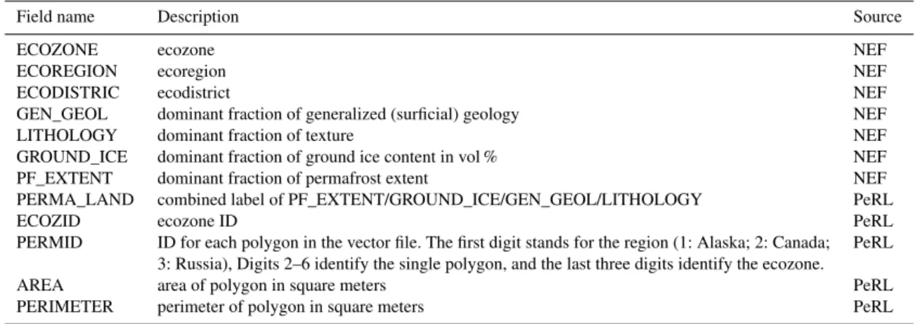
Table B2.Description of attributes contained in the polygon attribute table of Canadian permafrost landscapes (canada_perma_land.shp).

ECOZONE ecozone NEF

ECOREGION ecoregion NEF

ECODISTRIC ecodistrict NEF

GEN_GEOL dominant fraction of generalized (surficial) geology NEF

LITHOLOGY dominant fraction of texture NEF

GROUND_ICE dominant fraction of ground ice content in vol % NEF

PF_EXTENT dominant fraction of permafrost extent NEF

PERMA_LAND combined label of PF_EXTENT/GROUND_ICE/GEN_GEOL/LITHOLOGY PeRL

PERMID ID for each polygon in the vector file. The first digit stands for the region (1: Alaska; 2: Canada; PeRL 3: Russia), Digits 2–6 identify the single polygon, and the last three digits identify the ecozone.

Table B3.Description of attributes contained in the polygon attribute table of Russian permafrost landscapes (russia_perma_land.shp).

ECOZONE metadata: http://maps.tnc.org/ Olson et al. (2001), downloaded at http://maps.tnc.org/gis

GEN_GEOL surficial geology LRR; Stolbovoi and McCallum (2002)

LITHOLOGY texture LRR; Stolbovoi and McCallum (2002)

GROUND_ICE ground ice content in vol % LRR

PF_EXTENT permafrost extent LRR

PERMA_LAND combined label of LRR

PF_EXTENT/GROUND_ICE/GEN_GEOL/LITHOLOGY

PERMID ID for each polygon in the vector file. The first digit stands for PeRL

the region (1: Alaska; 2: Canada; 3: Russia), digits 2–6 identify the single polygon, and the last three digits identify the ecozone.

Table B4. Terminology for permafrost properties in the regional permafrost databases of Alaska (AK2008), Canada (NEF), and Rus-sia (LRR).

Description PeRL AK2008 NEF LRR