Any correspondence concerning this service should be sent
to the repository administrator:
[email protected]
This is an author’s version published in:
http://oatao.univ-toulouse.fr/22522
To cite this version:
Cruz Cavalcanti, Yanna and Oberlin, Thomas and
Dobigeon, Nicolas and Stute, Simon and Ribeiro, Maria and Tauber,
Clovis Unmixing dynamic PET images with variable specific binding
kinetics. (2018) Medical Image Analysis, 49. 117-127. ISSN 1361-8415
Official URL
DOI :
https://doi.org/10.1016/j.media.2018.07.011
Open Archive Toulouse Archive Ouverte
OATAO is an open access repository that collects the work of Toulouse
researchers and makes it freely available over the web where possible
Unmixing
dynamic
PET
images
with
variable
specific
binding
kinetics
s
Yanna
Cruz
Cavalcanti
a, ∗,
Thomas
Oberlin
a,
Nicolas
Dobigeon
a, b,
Simon
Stute
c,
Maria
Ribeiro
d,
Clovis
Tauber
da IRIT/INP-ENSEEIHT Toulouse, University of Toulouse, BP 7122, 31071 Toulouse Cedex 7, France b Institut Universitaire de France, France
c UMRS Inserm U1023 IMIV-CEA SHFJ, Orsay, 91400, France d UMRS Inserm U930 – Université de Tours, Tours, 37032, France
Keywords: Dynamic PET image Unmixing Brain imaging Factor analysis Matrix factorization NMF
a
b
s
t
r
a
c
t
Toanalyzedynamicpositronemissiontomography(PET)images,variousgeneric multivariatedataanal- ysistechniques have beenconsideredintheliterature,suchasprincipal componentanalysis(PCA),inde-pendentcomponent analysis(ICA), factor analysisand nonnegativematrixfactorization(NMF).Neverthe-less,theseconventionalapproachesneglectanypossible nonlinearvariations inthe timeactivitycurves describingthekineticbehavioroftissueswithspecificbinding,whichlimits theirability torecoverareli-able,understandableand interpretabledescriptionofthedata.Thispaperproposesan alternativeanalysis paradigmthataccountsforspatialfluctuationsinthe exchangerateofthetracerbetweenafree compart-mentandaspecificallyboundligandcompartment. Themethodreliesontheconceptoflinearunmixing, usuallyappliedon thehyperspectraldomain,whichcombinesNMFwithasum-to-oneconstraintthat en-suresanexhaustivedescriptionofthe mixtures.Thespatialvariabilityofthesignature correspondingto thespecificbindingtissueisexplicitlymodeledthrougha perturbedcomponent.Theperformance ofthe methodisassessedonbothsyntheticandrealdataandisshownto compete favorablywhencompared tootherconventionalanalysismethods.
1. Introduction
Dynamicpositronemissiontomography(PET)isanon-invasive nuclear imaging technique that allows biological processes to be quantified andorgan metabolicfunctionstobeevaluated through the three-dimensional measure of the radiotracer concentration overtime.
TheanalysisofdynamicPETimages,inparticularthe quantifi-cationofthekineticpropertiesofthetracer,requirestheextraction of tissue time-activity-curves(TACs) inorder to estimate the pa-rameters fromcompartmental modeling(Innis ,2007). Neverthe-less,PETimagesarecorruptedbyaprominentstatisticalnoiseand elementary TACs are mixed up due to the partial volume effect. Therefore, inferring rigorousand reliable information from these imagesstillremainsachallengingissue.
s Part of this work has been supported by CAPES. ∗ Corresponding author.
Several generic methods have been applied to estimate ele-mentary TACsandtheir corresponding proportions fromdynamic PET images. These techniques have different denominations de-pending on the application context,but all aim attackling blind source separation(BSS)problems.Forinstance,Barber(1980) and
Cavailloles (1984) proposed matrixfactorization-based PET analy-sis techniques,referredtoasfactoranalysisofdynamic structures (FADS)(Chou,2007).AnimprovementofFADStakingintoaccount thenonnegativephysiologicalcharacteristicofPETimageswas pro-posed subsequently by Wu (1995) andSitek (2000), also appear-ing in other biomedical imaging domains (Martel , 2001). Non-negative matrix factorization (NMF) techniques pursue the same objective, under nonnegativity constraints on the latent factors to be recovered, and have been intensively applied in dynamic PET studies (Lee, 2001;Padilla ,2012; Schulz,2013). The works of Sitek (2002) and El Fakhri(2005) improved nonnegativeFADS withapenalizationthatpromotednon-overlappingregionsineach voxel.
The approachproposed in thispaperfollowsthesame lineas NMFornonnegativeFADS.ItaimsatdecomposingeachPETvoxel TACintoaweightedcombinationofpurephysiologicalfactors, rep-resentingtheelementaryTACassociatedwiththedifferenttissues present within thevoxel.This factormodelingisenriched witha
E-mail addresses: [email protected] (Y.C. Cavalcanti), thomas.oberli [email protected] (T. Oberlin), [email protected] (N. Dobigeon), simon.st [email protected] (S. Stute), [email protected] (M. Ribeiro), clovis.tauber@univ- tours.fr (C. Tauber).
C
F +N S
C
S
C
P
Tissue
k
1k
2k
3k
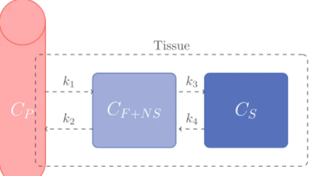
4Fig. 1. Configuration of the classic three-compartment kinetic model used in many imaging studies.
sum-to-one constraintto thefactorproportions, sothat they can be interpreted astissue percentages within eachvoxel. In partic-ular, this additional constraintexplicitly solves the scaling ambi-guity inherent toanyNMF models,whichhas provento increase robustness aswellasinterpretability.ThisBSStechnique, referred toasunmixingorspectralmixtureanalysis,originatesfromthe geo-science and remote sensing literature (Bioucas-Dias , 2012) and has proven its interest in other applicative contexts, such as mi-croscopy(Huang,2011)andgenetics(DobigeonandBrun,2012).
Thelinearityassumptionforvoxeldecompositionunderlinedby the above-mentioned PET analysis methods can be envisionedin thelightofcompartmentmodeling,atoolwidelyemployedto de-scribe thekinetic behavior occurringwithin thevoxel.The selec-tion ofa given model should be based on the radiotracer under study(Gunn,1997;Innis,2007)butmostofthemodelsconsider that themeasuredsignal inagivenvoxelisthesumofthe com-prisingcompartments.
However, factor TACs to be recovered cannot always be as-sumed to haveconstant kinetic patterns,as implicitlyconsidered in conventional methods. Fig.1 depictsan example ofa 2-tissue compartmentalmodel,wheretheradioligandisassumedtomove between threecompartments: Cp represents theradioligand con-centration inarterial plasma,CF+NS represents thefree plus non-specific compartment, and CS represents the specifically bound compartment. The exchange between compartments are subject to rateconstants kj (j=1,...,4) (Häggström,2016). Considering boththe2-tissueandreferencecompartmentmodels,the assump-tion ofconstant kinetic patterns seemsappropriate for theblood compartment as well as non-specific binding tissues, since they present somehomogeneitybesidessomeperfusiondifference(e.g. white matter versus graymatter). Therefore their contributionto the voxelTACshouldbe fairly proportionalto thefractionofthis type oftissue in the voxel.However, things getdifferent regard-ing thespecific bindingclass,astheTACassociatedwiththis tis-sue isnonlinearlydependent onboth theperfusion andthe con-centrationoftheradiotracer target.Thespatialvariationontarget concentration is inpartgovernedby differencesinthe k3 andk4
kineticparameters,whichnonlinearlymodifytheshapeoftheTAC characterizing thisparticularclass.Muzi(2005) discussedthe ac-curacy ofparameter estimatesfor tumor regions and underlined higherrorsfortheparameters relatedtospecificbinding,namely 26% fork3 and49% for k4. Theseresults were further confirmed bySchiepers(2007).Morespecifically,theystudiedthekineticsof lesioned regionsthatwere tumorandtreatmentchange predomi-nant,showingthatvariationsonk3 andk4mayallowfor differen-tiation.Bai(2013) furtherdiscussednonuniformityinintratumoral uptakeanditsimpactonpredictingtreatmentresponseandtumor aggressiveness.Nonetheless, thisfluctuationphenomenon hasnot
been taken into account by the decomposition models from the literature.
Themain motivationofthispaperisto proposea more accu-ratedescription ofthe tissues andkinetics composing thevoxels indynamic PETimages,inparticularforthoseaffectedbyspecific binding. To this end, this work proposesto explicitly model the nonlinearvariabilityinherenttotheTACcorrespondingtospecific binding,byallowingthecorrespondingfactortovaryspatially.This variationisapproximatedbyalinearexpansionovertheatomsof adictionary,whichhavebeenlearnedbeforehandbyconductinga principalcomponentanalysisonalearningdataset.
The sequel of this paper is organized as follows. The pro-posed mixing-based analysis model is described in Section 2.
Section 3 presentsthe corresponding unmixingalgorithm ableto recoverthefactors,their corresponding proportionsineach voxel and the variability maps. Section 4 details synthetic data gener-ation and real data acquisition. Simulation results obtained with syntheticdataandexperimental resultsonrealdataare reported inSection5.Section7 concludesthepaper.
2. Method
2.1. Specificbindinglinearmixingmodel(SLMM)
ConsiderNvoxelsofa3DdynamicPETimageacquiredatL suc-cessivetime-frames.First,weomitthespatialblurringinducedby the point spread function (PSF) ofthe instrument and any mea-surementnoise.TheTACinthenth voxel(n∈
{
1,...,N}
)over theLtime-framesisdenotedxn=[x1,n,...,xL,n]T.AkintovariousBSS techniquesand following the linearmixing model(LMM) for in-stanceadvocatedinthePETliterature byBarber(1980),each TAC
xn is assumedto be alinear combinationofK elementaryfactors
mk xn= K X k=1 mkak,n (1)
wheremk=[m1,k,...,mL,k]T denotesthe pure TACofthe kth tis-suetypeandak,n isthefactorproportionofthekthtissueinthe
nthvoxel. The factors mk (k=1,...,K) correspond to the kinet-icsofthe radiotracer inaparticular type oftissue inwhichthey aresupposedspatiallyhomogeneous.Forinstance,theexperiments conductedinthisworkanddescribedinSections4.1 and4.2 con-sider3typesoftissues thatfallintothiscategory:the blood,the non-specificgraymatterandthewhitematter.
Additionalconstraints regardingthesesets ofvariablesare as-sumed.First, since the elementaryTACs are expected tobe non-negative,thefactorsareconstrainedas
ml,k≥0,
∀
l,k. (2)Moreover,nonnegativity andsum-to-one constraintsare assumed forallthefactorproportions(n=1,...,N)
∀
k∈{
1,...,K}
, ak,n≥0 and KX
k=1
ak,n=1. (3) Foragivenvoxelindexedbyn,thissum-to-oneconstraint(3) en-forcesthemixingcoefficientsak,n (k=1,...,K)tobe interpreted asconcentrations(Keshava,2003).
Moreimportantly,whenfactorsareaffectedbypossibly nonlin-ear andspatially varying fluctuationswithin the image, the con-ventionalNMF-like linearmixingmodel (1) no longerprovides a sufficient description of data.Therefore, over recent years, factor variabilityhasreceivedincreasedinterestinthehyperspectral im-ageryliteratureasitallowschangesonlighteningandenvironment tobe taken intoaccount (Zare andHo, 2014;Halimi ,2015). Re-cently,Thouvenin(2016) haveproposedaperturbedLMM(PLMM)
tofurtheraddressthisproblem.Inthedynamic PETimage frame-work, factorvariabilityisexpectedtomainlyaffecttheTAC asso-ciated withspecific binding,denotedm1,whilethepossible
vari-abilitiesintheTACsmk(k∈
{
2,...,K}
)relatedtotissuesdevoidofa specifically bound compartment are supposed weaker and ne-glected in this study. Since this so-called specific binding factor (SBF)isassumedtovaryspatially,itwillbespatiallyindexed.Thus, adapting the PLMMapproach toour problem, theSBFin agiven voxelwill be modeledasa spatially-variantadditive perturbation affectinganominalandcommonSBFm¯1
m1,n=m¯1+
δm
1,n (4) wheretheadditivetermδ
m1,ndescribesitsspatialvariabilityover the image. However, recovering the spatial fluctuationδ
m1,n in each image voxel is a high-dimensional problem. To reduce this dimensionality,thevariationswillbeassumedtolie insidea sub-space of small dimension Nv≪L. As a consequence, similarly to the strategy followed by Park (2014), the additive termsδ
m1,n (n∈{
1,...,N}
)aresupposedtobeapproximatedbythelinearex-pansion
δm
1,n= Nv X i=1 bi,nvi, (5)wherethe Nv variabilitybasiselements v1,...,vNv canbe chosen beforehand,e.g.,byconductingaPCAonalearning setcomposed of simulated or measured SBFs. The PCA aims at extracting the mainvariabilitypatterns,whileallowing fordimension reduction. Thus, the setof coefficients
©
b1,n,...,bNv,nª
quantifythe amountofvariabilityinthenthvoxel.ThenominalSBFm¯
1isalsoroughly
estimatedfromthelowestvaluesofthisdatasetandfurtherfixed so thatall thevariabilitycoefficientsare nonnegative,inorderto reduce correlationbetweenthevariabilityelementsandtheother tissuefactors.
Combiningthelinearmixingmodel(1),theperturbationmodel
(4)andits linearexpansion (5),the voxelTACs aredescribed ac-cording to the following so-called specific binding linear mixing model(SLMM) xn=a1,n
³
¯ m1+ Nv X i=1 bi,nvi´
+ K X k=2 ak,nmk. (6) To be fully comprehensive and motivated by the findings ofHenrot(2014),thisworkalsoproposestoexplicitlymodelthePET scan point spreadfunction(PSF),combininga deconvolutionstep jointlywithparameterestimation.WewilldenotebyHthelinear operator that computesthe 3D convolution by some knownand spatiallyinvariantPSF,whichleadsto
Y=MAH+
h
E1A◦VBi
H|
{z
}
1 +R (7)where M=[m¯1,...,mk] is a L×K matrix containing the factor TACs,A=[a1,...,an]isaK×Nmatrixcomposedofthefactor pro-portionvectors,“◦” isthe Hadamardpoint-wiseproduct,E1isthe matrix[1L,10L,K−1],V=[v1,...,vNv]istheL×Nvmatrixcontaining thebasiselementsusedtoexpandthespatialvariabilityoftheSBF,
B=[b1,...,bn]is the Nv×N matrixcontaining the intrinsic pro-portions, and R=[r1,...,rN]T is the L×N matrix accountingfor noise and mismodeling. Notethat ifB=0 andH=I,the model in (7) reduces tothe conventional linear mixingmodelgenerally assumedbyfactormodeltechniqueslikeNMFandICA.
Whilenoisesassociatedwithcountratesaretraditionally mod-eled by a Poisson distribution (Shepp andVardi, 1982), postpro-cessingcorrectionsandfilteringoperatedbymodern PETsystems significantly alter thenature ofthe noise corruptingthe final re-constructed images. Modeling the noise on this final data is a
highlychallengingtask(Wilson,1994).However,asdemonstrated by Fessler (1994), pre-corrected PET data can be sufficiently ap-proximated by a Gaussian distribution. As a consequence,in this work, the noise vectors rn=[r1,n,...,rL,n] (n∈
{
1,...,N}
) are as-sumed tobenormallydistributed.Moreover,withoutloss of gen-erality, all vector components rℓ,n (ℓ=1,...,L and n=1,...,N) will be assumed to be independent and identically distributed. This assumption seems to evade anyspatial andtemporal corre-lations thatmaycharacterizethe noisegenerallyaffectingthe re-constructedPETimages(Tichý andŠmídl,2015).However,the pro-posedmodelcanbeeasily generalizedtohandlecolorednoiseby weighting the modeldiscrepancymeasure accordingto thenoise covariance matrix, asdone by Fessler (1994). Alternatively, after diagonalizingthenoisecovariancematrix,thePETimagetobe an-alyzed canundergoa conventionalwhitening pre-processingstep (Thireou,2006;Bullmore,2001;Turkheimer,2003).Inadditiontothenonnegativityconstraintsappliedtothe ele-mentary factors (2) and factorproportions (3),the intrinsic vari-ability proportion matrix B is also assumed to be nonnegative, mainlytoavoidspuriousambiguity,i.e.,
Bº0Nv,N, (8)
where 0Nv,N denotes theNv×N-matrixmadeof0’sandº stands for acomponent-wise inequality.We accordinglyfix the nominal SBF m¯1 with a robust estimation of the TAC chosen asa lower bounding signature ofa set ofpreviously generated ormeasured SBFTACs.Capitalizingonthismodel,theunmixing-basedanalysis ofdynamicPETimagesisformulatedinthenextparagraph.
2.2. Problemformulation
TheSLMM(7) andconstraints(2),(3) and(8) canbecombined to formulate a constrained optimizationproblem. In order to es-timate the matrices M, A, B, a proper cost function is defined. The data-fitting term is defined as the Frobenius norm
k
·k
2F of the difference between the dynamic PET image Y and the pro-posed data modelingMAH+1
. Thiscorresponds to the negativelog-likelihood underthe assumption ofGaussian noise.Since the problem is ill-posed and non-convex, additional regularizers be-come essential. In this paper, we propose to define penalization functions
8
,9
andÄ
to reflecttheavailable a priori knowledge onM,AandB,respectively.Theoptimizationproblemisthen de-finedas(
M∗,A∗,B∗)
∈argmin M,A,Bn
J(
M,A,B)
s.t.(
2)
,(
3)
,(
8)
o
(9) with J(
M,A,B)
= 1 2°
°
°
Y−MAH−h
E1A◦VB)
i
H°
°
°
2 F +α
8(
A)
+β
9 (
M)
+λ
Ä(
B)
(10)where the parameters
α
,β
andλ
control the trade-off between thedatafittingtermandthepenalties8
(A),9
(M) andÄ
(B), de-scribedhereafter.2.2.1. Factorproportionpenalization
Thefactorproportionsrepresentingtheamountofdifferent tis-suesareassumedtobespatially smooth,sinceneighboringvoxels maycontainthesametissues.Wethuspenalizetheenergyofthe spatialgradient
8(
A)
=12
k
ASk
2F, (11)whereSistheoperatorcomputingthefirst-orderspatialfinite dif-ferences.MoredetailsarereportedbyCavalcanti(2017).
2.2.2. Factorpenalization
The chosenfactorpenalizationbenefitsfromtheavailabilityof rough factorTACsestimatesM0=
£
m¯10,. . .,m0K¤
.Thus,wepropose to enforce similarity (in termof mutualEuclidean distances) be-tweentheseprimaryestimatesandthefactorTACstoberecovered9 (
M)
= 1 2°
°M
−M0°
°
2F. (12)2.2.3. Variabilitypenalization
The SBFvariability is expectedto affect only a small number of voxels, thosebelonging to theregion containing the SBF.As a consequence,weproposetoenforcesparsityviatheuseoftheℓ1
-norm,alsoknownastheLASSOregularizer(Tibshrani,1996)
Ä(
B)
=k
Bk
1 (13)where
k
.k
1istheℓ1norm.Thispenaltyforcesbi,ntobe0outside thehigh-uptakeregion,thusreducingoverfitting.3. Algorithmimplementation
Given the nature of the optimization problem (9), which is genuinely nonconvex and nonsmooth, the adopted minimization strategyreliesontheproximalalternatinglinearizedminimization (PALM)scheme(Bolte,2013).PALMisan iterative,gradient-based algorithm which generalizes the Gauss-Seidel method. It consists in iterative proximal gradient steps with respect to A, M and B
and ensures convergence to a local critical point A∗,M∗ and B∗.
The principleofPALMisbrieflyrecalledbyCavalcanti(2017).Itis specificallyinstantiatedfortheunmixing-basedkineticcomponent analysis considered in this paper. The resulting SLMM unmixing algorithm, whosemainsteps aredescribed inthefollowing para-graphs,issummarizedinAlgorithm1.
Algorithm1:SLMMunmixing:mainalgorithm.
Data:Y
Input:A0,M0,B0
1k←0;
2whilestoppingcriterionnotsatisfieddo
3 Mk+1←P+
³
Mk− γ Lk M∇
MJ(
Mk,Ak+1,Bk)
´
4 Ak+1←PAR³
Ak− γ Lk A∇
AJ(
Mk,Ak,Bk)
´
5 Bk+1← proxλ Lk B k.k1³
P+³
Bk− γ Lk B∇
BJ(
Mk+1,Ak+1,Bk)
´´
6 k←k+1 7A←Ak+1 8M←Mk+1 9B←Bk+1 Result:A,M,B3.1. OptimizationwithrespecttoM
A direct application of the approach presented by
Bolte (2013) under the constraints defined by (2) leads to the followingupdatingrule
Mk+1=P +
³
Mk− 1 Lk M∇
MJ(
Mk,Ak+1,Bk)
´
(14)whereP+
(
·)
istheprojector ontothenonnegativeset{X|Xº0L,R} andtherequiredgradientwrites∇
MJ(
M,A,B)
=(
(
E1A◦VB)
H−Y)
HTAT+M
(
AHHTAT)
+β
(
M−M0)
. (15)3.2.OptimizationwithrespecttoA
SimilarlytoSection3.1,thefactorproportionupdateisdefined asthefollowing Ak+1=P AR
³
Ak− 1 Lk A∇
AJ(
Mk,Ak,Bk)
´
, (16)wherePAR
(
·)
istheprojectiononthesetARdefinedbythefactor proportionconstraints (3), whichcan be computed withefficient algorithms,see,e.g., thework ofCondat(2015). Thegradientcan becomputedas∇
AJ(
M,A,B)
=−MT(
DA)
−ET1(
DA◦VB)
+αASS
T withDA=(
Y−MAH−(
E1A◦VB)
H)
HT.3.3.OptimizationwithrespecttoB
Finally,theupdatingruleforthevariabilitycoefficientscanbe writtenas Bk+1=prox λ Lk B k.k1
³
P+³
Bk− 1 Lk B∇
BJ(
Mk+1,Ak+1,Bk)
´´
,wheretheproximalmappingoperatoristhesoft-thresholding op-erator. Indeed, the proximal map ofthe sum of the nonnegative indicator function andtheℓ1 norm is exactlythe composition of
theproximalmapsofbothindividualfunctions,followingthesame principleshowedbyBolte(2013).Thegradientwrites
∇
BJ(
M,A,B)
=VT¡
(
E1A)
◦(
−Y+MAH+1)
HT¢
.4. Experimentaldesign
4.1. Syntheticdatageneration
Toillustratetheaccuracyofouralgorithm,experimentsarefirst conducted on synthetic data for which the ground truth of the mainparametersofinterest(i.e.,factorTACsandfactorproportion maps)isknown.IntheclinicalPETframework,groundtruth con-cerningthetracerkineticsanduptakeisnevercompletelyknown. Meanwhile, simulations benefit from an entire knowledge ofthe patientpropertiesandkinetics,andtheirdegreeofcomplexityand detailscanbeselectedaccordingtothepurposeofthestudy. Fur-thermore, several simulations can be performed in a reasonable time.
Thus, experimentations are conducted on set of 20 syn-thetic images of size 128×128×64. As in Boellaard (2008) and
Yaqub (2012), each image voxel is constructed as a combination ofK=4pureTACsrepresentativeofthebrain,whichistheorgan ofinterestinthepresentwork:specificgraymatter,purebloodor veins,purewhitematterandnon-specificgraymatter.First,ahigh resolutiondynamicPETnumericalphantomwithlabeledregionsof interest(ROIs)(Stute,2015),hasbeenused tocreatetheground truth for factor and proportions. In this phantom, all the distri-butions of thetracer per region have beenextracted froma real dynamic PET image acquiredinL=20times ofacquisition rang-ing from1 to 5 min ina totalperiod of 60min. For thisstudy, the patient was injected with the [11C]PE2I radioligand. Using a phantomextracted fromPET acquisitionsof a realpatient brings to the syntheticimage the complexity of real data.For instance, thepureTACsconstitutiveofthisphantomimagearecreatedfrom theaveragingofvisuallysegmentedregionsandthereforearestill mixed up due to partial volume. To simulate realistic variability of the SBF, a set of synthetic TACs generated through a realistic compartment-based modelis used.More details can be found in thetechnicalreportofCavalcanti(2017).
0
1000
2000
3000
4000
Time
0
0.05
0.1
0.15
0.2
0.25
0.3
0.35
Variability basis element
0
1000
2000
3000
4000
Time
0
20
40
60
80
Concentration
Specific Binding TACs
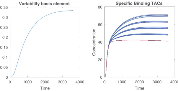
Fig. 2. Left: variability basis element v 1 identified by PCA. Right: generated SBFs (blue) and the nominal SBF signature (red). (For interpretation of the references to color in this figure legend, the reader is referred to the web version of this article.)
• Followinga2-tissuecompartment-basedmodel(Phelps,1986),
alarge databaseofSBFTACshasbeengeneratedby randomly varyingthek3parameter(representingthespecificbindingrate
oftheradiotracer inthetissue). APCAwasconductedonthis dataset,andananalysisoftheeigenvaluesledtothechoiceof auniquevariabilitybasiselementV=v1(i.e.,Nv=1),depicted
inFig.2 (left).
• The nominalSBF TAC ¯m1 is then chosen asthe TAC of
mini-mum area underthe curve (AUC) amongall theTACs ofthis database.ThisTACisdepictedinFig.2 (right,redcurve).
• The dynamic PET phantom has been linearly unmixed
us-ing the N-FINDR (Winter, 1999) and SUnSAL ( Bioucas-Dias and Figueiredo, 2010) algorithms to select the ground-truthnon-specificfactorTACm2,...,mKandfactorproportions
a1,...,aN, respectively. These factor TACs and corresponding factorproportionmapsare depictedinFig.3 (top)andFig.4, respectively.
• The 1st row of the factor proportion matrix A, namely A1,
£
a1,1,...,a1,N
¤
was designed to locate the region associated withspecific binding. Then,the Nv×N matrix B=[b1,...,bN] mappingthe SBFvariabilityineach voxel hasbeenartificially generated. The high-uptake region was divided into 4 subre-gions with non-zero coefficients bn, asshown in Fig. 5 (left), whilethesecoefficientsaresettobn=0outsidetheregion af-fectedwithSBF.Ineachofthesesubregions,thenon-zero coef-ficientsbnhavebeendrawnaccordingtoGaussiandistributions withaparticularmeanvalueandsmallvariances.The spatially-varying SBFs in each region are then generated according to themodel in(5) and(4).Some resultingtypical SBFTACs are showedinFig.2.Afterthisprimarygenerationprocess,aPSFdefinedasa space-invariant andisotropicGaussianfilterwithFWHM=4.4mmis ap-plied to the output image. In brain imagingusing a clinical PET scanner,thisisanacceptableapproximation,sincethedegradation of thescanner resolution mainlyaffects the bordersof the field-of-view (Rahmim,2013;Mehranian,2017). Finallythe measure-ments havebeencorruptedbya zero-meanwhiteGaussian noise withasignal-to-noiseratioSNR=15dB,inagreementwitha pre-liminarystudyconductedontherealistic replicasofStute (2015), which showed that the SNR ranges from approximately 10dB on the earlierframes to 20dB on the latter ones. Simulations were
conducted in20different realizationsof thenoise to getreliable performancemeasures.
4.2. Realdataacquisition
Toassessthebehavioroftheproposedapproachwhen analyz-ingrealdynamicPETimages,thedifferentmethodshavebeen ap-pliedtoa dynamicPETimage with[18F]DPA-714 ofastroke sub-ject.Cerebralstrokeisasevereandfrequentlyoccurringcondition. While differentmechanisms areinvolved inthestroke pathogen-esis, thereisanincreasingevidencethatinflammation,mainly in-volving the microglial andthe immune systemcells, account for itspathogenicprogression.The[18F]DPA-714isaligandofthe 18-kDa translocator protein (TSPO) for in vivo imaging, which is a biomarkerofneuroinflammation.Thesubjectwasexaminedusing anIngenuityTOFCamerafromPhilipsMedicalSystems,sevendays afterthestroke.
The PET acquisition was reconstructed into a 128×128× 90-voxels dynamic PET image with L=31 time-frames. The PET scan image registration time ranged from 10 s to 5 min over a 59 min period. The voxel size was of 2×2×2 mm3. As for the experiments conducted on simulated data, once again as in
Boellaard (2008) andYaqub(2012),the voxelTACs havebeen as-sumed to bemixtures ofK=4 typesofelementary TAC:specific bindingassociatedwithinflammation,blood,thenon-specificgray and whitematters. The K-means methodwas applied to the im-ages to mask the cerebrospinal fluid andto initialize NMF, LMM and SLMM algorithms. A groundtruth of the high-uptake tissue wasmanuallylabeledbyanexpertbasedonamagneticresonance imaging (MRI) acquisition. The stroke region was segmented on thisregisteredMRIimagetodefineasetofvoxelsusedtolearnthe variability descriptorsV by PCA.The nominalSBFhas beenfixed astheempiricalaverageofthecorrespondingTACswithAUC com-prised betweenthe5thand10thpercentile.Thechoicetousethe average ofa percentileinsteadoftheminimumAUC TACis moti-vatedbythefactthat,inthiscase,thelearningsetiscorruptedby noiseandpartialvolumeeffects.
4.3. Comparedmethods
The resultsofthe proposed algorithmhavebeen comparedto thoseobtainedwithseveralclassicallinearunmixingmethodsand
Ground truth
0
0.5
1
Kmeans
0
0.5
1
NMF
0
0.5
1
VCA
0
0.5
1
LMM
0
0.5
1
SLMM
0
0.5
1
0
0.5
1
0
0.5
1
0
0.5
1
0
0.5
1
0
0.5
1
0
0.5
1
0
0.5
1
0
0.5
1
0
0.5
1
0
0.5
1
0
0.5
1
0
0.5
1
0
0.5
1
0
0.5
1
0
0.5
1
0
0.5
1
0
0.5
1
0
0.5
1
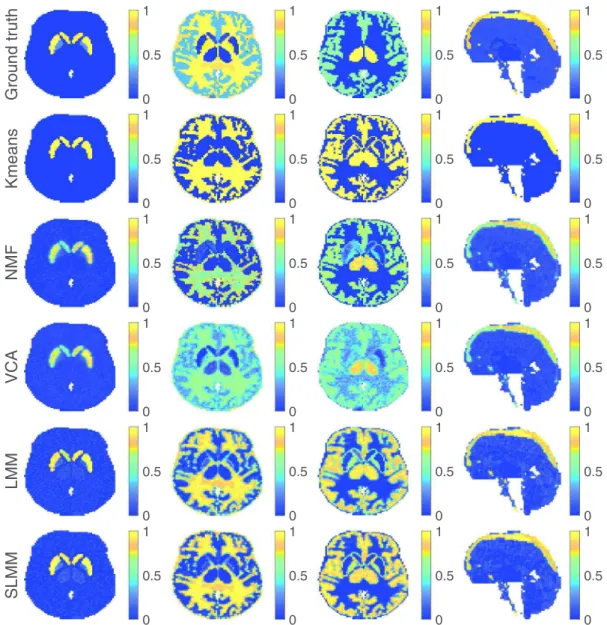
Fig. 3. Factor proportion maps of the 15th time-frame obtained for SNR = 15dB corresponding to the specific gray matter, white matter, gray matter and blood, from left to right. The first 3 columns show a transaxial view while the last one shows a sagittal view. All images are in the same scale in [0,1].
other BSStechniques.The methods arerecalledbelow withtheir mostrelevantimplementationdetails.
NMF(novariability).TheNMFalgorithmhereinappliedisbased onmultiplicativeupdaterulesusingtheEuclideandistanceascost function (Leeand Seung, 2000). The stopping criterion is set to 10−3. To obtain a faircomparison mitigating scale ambiguity
in-herenttomatrixfactorization-likeproblem,resultsprovidedbythe NMF havebeennormalizedbythemaximumvalue forthe abun-dance,i.e., ˆ Ak← ˆ Ak
°
°
Aˆk°
°
∞ ˆ mk←mˆk°
°
Aˆk°
°
∞ (17)where Aˆkdenotes thekthrowofthe estimatedfactorproportion matrixAˆ.
VCA(novariability).ThefactorTACsarefirstextractedusingthe vertexcomponentanalysis(VCA)whichrequirespurevoxelstobe present intheanalyzed images(NascimentoandDias, 2005).The factorproportionsaresubsequentlyestimatedbysparseunmixing byvariablesplittingandaugmentedLagrangian(SUnSAL)( Bioucas-DiasandFigueiredo,2010).
LMM (no variability)LMM(novariability).Toappreciatethe in-terestofexplicitlymodelingthespatialvariabilityoftheSBF,a
de-Table 1
Factor proportion, factor and variability penaliza- tion parameters for LMM and SLMM. LMM SLMM α 0.010 0.010 β 0.010 0.010 λ – 0.020 ε 0.001 0.001
preciated version oftheproposed SLMMalgorithm isconsidered. Moreprecisely,itusestheLMM(1) withoutallowingtheSBFm1,n tobespatially varying.Thestoppingcriterion, definedas
ε
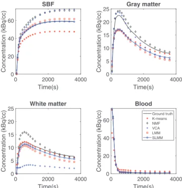
,isset to10−3.Thevaluesoftheregularizationparameterarereportedin Table1.SLMM(proposedapproach).AsdetailedinSection2.1, ma-trixBisconstrainedtobe nonnegativeto increaseaccuracy. Con-sequently,thenominalSBFTAC m¯1 isinitializedasthe TACwith theminimumAUClearnedfromthegenerateddatabasetoensure apositiveB.TheregularizationparametershavebeentunedtotheSBF 0 2000 4000 Time(s) 0 20 40 60 Concentration (kBq/cc) White matter 0 2000 4000 Time(s) 0 5 10 15 20 25 Concentration (kBq/cc) Gray matter 0 2000 4000 Time(s) 0 5 10 15 20 25 Concentration (kBq/cc) Blood 0 2000 4000 Time(s) 0 20 40 60 Concentration (kBq/cc) Ground truth K-means NMF VCA LMM SLMM
Fig. 4. TACs obtained for SNR = 15 dB. For the proposed SLMM algorithm, the repre- sented SBF TAC corresponds to the empirical mean of the estimated spatially vary- ing SBFs m 1,1 , . . . , m 1,N .
Fig. 5. Ground-truth (left) and estimated (right) SBF variability.
valuesreportedinTable1.Asfortheother approaches, the stop-pingcriterionissetto10−3.
Since the addressed problem is non-convex, thesealgorithms requirean appropriate initialization.Inthiswork,the factorTACs have been initialized as the outputs M0 of a K-means clustering conducted on the PET image. TheseK-means TACs estimates are alsoconsideredforperformancecomparison.
Theperformance ofthealgorithmsonsyntheticdatahasbeen accessed through the use of a normalized mean square error (NMSE)computedforeachvariable
NMSE
(
θ
ˆ)
=k
ˆ
θ
−θk
2F
k
θk
2F (18)where
θ
ˆistheestimatedvariableandθ
thecorrespondingground truth. The NMSE has been measured for the following parame-ters: the factor proportions A1 corresponding to the high-uptake region,theremainingfactorproportionsA2:K,theSBFsaffectedby the variabilityM˜1,[m1,1,...,m1,N],the non-specific factorTACsM2:K,[m2,...,mK] and finally the variability factor proportion matrixB.
4.4. Hyperparametertuning
Considering the significant number of hyperparameters to be tuned in both LMM andSLMM approaches (i.e.,
α
,β
,λ
), a fullsensitivityanalysisisachallengingtask,whichisfurther complex-ifiedbythenon-convexnatureoftheproblem.Toalleviatethis is-sue,eachparameterhasbeenindividuallyadjustedwhilethe oth-ershavebeensettozero.Severalsimulations empiricallyshowed that the resultis not very sensitive to the choice of parameters. Theparametershavebeentuned suchthatthetotalpercentageof theircorrespondingtermintheoverallobjectivefunctiondoesnot surpass25%ofthetotalvalueofthefunction.Giventhehighlevel ofnoise corruptingthePETimages,thehyperparameter
α
associ-ated withthefactorproportionshasbeensetsoastoreducethe noise impact whileavoidingtoomuch smoothing.ThefactorTAC penalization hyperparameterβ
results from a trade-off between the quality of the initial factor TAC estimates M0 andthe flexi-bility requiredbyPALM toreach moreaccurate estimates.Finally the variability penalizationλ
has been tuned to achieve a com-promise between therisks of capturingnoise into the variability term (i.e., overfitting) andof losing information.While there are moreautomatizedwaystochoosethehyperparametervalues(e.g., usingcross-validation,gridsearch,randomsearchandBayesian es-timation),thesehyperparameterchoiceshaveseemed tobe suffi-cient toassesstheperformance oftheproposed method.The hy-perparameter valuesusedinLMM andSLMMare finally reported inTable1.5. Results
5.1. Evaluationonsyntheticdata
The factor proportionmaps recovered by the compared algo-rithmsareshowninFig.3.Eachcolumncorrespondstoaspecific factor: SBF, white matter, non-specific gray matter, blood (from left toright,respectively).The sixrowscontainthefactor propor-tion maps ofthe groundtruth,andthose estimatedby K-means, NMF,VCA,LMMandtheproposed SLMM(fromtoptobottom, re-spectively). A visual comparison suggests that the factor propor-tionmapsobtainedwithLMMandSLMMaremoreconsistentwith the expected localization of each factor in the brain than VCA. Meanwhile, they are lessnoisy than the maps obtainedby NMF. TheestimatedLMMandSLMMproportionsmapsareclosertothe ground truth than both NMF andVCA, particularly inthe region affected by specific binding, as quantitatively shown in Table 2. It can alsobe observedthat thefactor proportionmaps obtained withtheproposedSLMMapproachpresentahighercontrast com-paredtoLMMandotherapproaches,especiallyinthehigh-uptake region.
The mapsof SLMMarealso sharpercompared toLMM. Addi-tionally, itisalsopossibletoseethatNMFresultsforwhite mat-ter are sharper but also more noisy than both LMM and SLMM approaches. However, forthespecific graymatter, bothLMM and SLMMapproachesshowsharperestimatedfactorproportionmaps. Note thatthesharpnessofthefactorproportionsisnot necessar-ily a good criterion of comparison. Indeed, factor analysis-based methods expect to recover smooth maps that take into account the spillingpartofpartial volumeeffect,whichisnot considered within deconvolution.Theaim ofunmixingisnothard-clustering orclassification.
The corresponding estimated factor TACs are shown in
Fig.4 where,forcomparisonpurposes,theSBFdepictedforSLMM is the empirical average over the whole set of spatially varying SBFs, as it is also the case for the SBF ground truth TACs. The best estimate of the SBF TAC seems to be obtained by the pro-posed SLMMapproach, forwhichthe TAC hasbeen precisely re-covered, asopposedtoK-means, VCAandNMF. K-meansprovide the best estimate of the white matter TAC, closely followed by SLMMwhileNMFhighlyoverestimatesit.Thebestestimateofthe non specificgraymatterTAChasbeenobtainedbyVCAandNMF,
Table 2
Normalized mean square errors of the estimated variables A1 , A2:K, M˜ 1 , M2:K and B for K-means, VCA, NMF, LMM and SLMM. A 1 A 2:K M˜1 M 2:K B K-means 0.567 0.669 0.120 0.442 − ± 4.3 ×10 −4 ± 2.2 ×10 −3 ±1.5 ×10 −4 ±6.1 ×10 −2 VCA 0.547 0.481 0.517 0.248 – ± 6.7 ×10 −4 ± 1.8 ×10 −3 ±9.3 ×10 −5 ±1.3 ×10 −3 NMF 0.512 0.558 0.517 0.133 – ± 1.0 ×10 −6 ± 3.8 ×10 −5 ±4.5 ×10 −5 ±1.5 ×10 −4 LMM 0.437 0.473 0.349 0.148 – ± 3.8 ×10 −6 ± 4.3 ×10 −8 ±6.0 ×10 −7 ±1.5 ×10 −6 SLMM 0.359 0.495 0.009 0.128 0.259 ± 1.3 ×10 −5 ± 3.1 ×10 −5 ±3.0 ×10 −8 ±9.8 ×10 −7 ± 2.3 ×10 −5
even though it is slightlyoverestimated. It can be observed that SLMM andLMM have underestimatedthis factorTAC, whichhas beencompensatedwithhighervaluesinthecorrespondingfactor proportionmap.The factorTACassociatedwithblood iscorrectly estimatedbySLMM,LMM,VCAandNMF.
Table2 presentstheNMSEoverthe20realizationsofthenoise for allalgorithms andvariables ofinterest.These quantitative re-sults confirm the preliminary findings drawn fromthe visual in-spection of Fig. 3 and 4. The proposed method outperforms all the othersfor the estimation of M˜1, M2:K and A
1.In particular,
SLMM provides a very precise estimation of the mean SBF TAC with an NMSE of 0.9%.In Fig. 4,the mean of theestimated SBF TACsm1,1,...,m1,NisveryclosetothegroundtruthforLMMand SLMMbutthe individualerrors computedforeach voxel demon-strate betterperformanceobtainedbySLMM. Italsoshowsbetter resultsthanK-meansandNMFforA2:K,eventhoughitisless ef-fectivebutstillcompetitivewhencomparedtoLMMandVCA.
TakingintoaccounttheSBFvariabilityallowstheestimationof
A1to beimprovedupto35%.Fig.5 comparestheactual
variabil-ityfactorproportionsandthoseestimatedbytheproposedSLMM. Thisfigureshowsthattheestimatednon-zeroscoefficientsare cor-rectlylocalizedinthe4subregionscharacterizedbysomeSBF vari-ability.Thesenon-zerovaluesseemtobeaffectedbysome estima-tion inaccuracies, mainly dueto the deconvolution.However, the estimationerrorstillstayscloseto25%.
5.2. Evaluationonrealdata
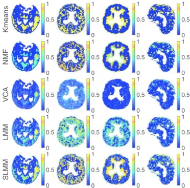
Fig. 6 depicts the factor proportion maps estimated by the compared methods. The corresponding estimatedfactor TACs are showninFig.7.TheLMMandSLMMalgorithmsestimatefour dis-tinct TACsassociatedwithdifferenttissues,asexpected. InFig.6, a remarkableresult is the factor proportion maps forthe blood. Thesagittalviewrepresentedinthelastrowisintheexactcenter ofthebrain.BothNMFandSLMMrecoverfactorproportionmaps that are invery good agreement withthe superior sagittal sinus vein that passeson thehigherpartofthebrain.Onthecontrary, VCAestimatestwofactorswhichseemtobemixturesofthevein TACsandotherregionTACs.
Fig.8 depictsthreedifferentviewsofthestrokeareaidentified by theexpertonMRIacquisition (1strow),theestimatedspecific gray matterfactor proportions(2nd–6th rows)andthe estimated corresponding variability(7throw).Allmethodsseemtocorrectly recoverthemainlocalizationofthestrokearea.However,the pro-posedSLMMapproachidentifiesasignificantlylargerarea.This re-sult seems to be in better agreement withthe stroke area iden-tified in the MRI acquisition of the same patient. Moreover, the specific gray matter factor proportion maps estimated by SLMM andK-meansshowhighvaluesinthethalamus,whichisaregion knowntopresentspecificbindingof[18F]DPA-714.Itispossibleto noteaninterestingimprovementofthefinalSLMMestimatewhen comparedtoitsK-meansinitialization.Thisdemonstratesthatthe
Kmeans
0 0.5 1NMF
0 0.5 1VCA
0 0.5 1LMM
0 0.5 1SLMM
0 0.5 1 0 0.5 1 0 0.5 1 0 0.5 1 0 0.5 1 0 0.5 1 0 0.5 1 0 0.5 1 0 0.5 1 0 0.5 1 0 0.5 1 0 0.5 1 0 0.5 1 0 0.5 1 0 0.5 1 0 0.5 1Fig. 6. Factor proportion maps of the real PET image with [ 18 F ]DPA-714 of a subject
with a stroke. The first 3 columns show a transaxial view while the last one shows a sagittal view. From left to right: the specific gray matter, white matter, non-specific gray matter and blood.
methodconvergestoan estimationofthespecificallybound gray matterthatismoreaccuratewiththeproposedmodel.
6. Discussion
6.1. Performanceofthemethod
This work proposes a novel unmixing method, called SLMM, that takes into account the spatial variabilityof high-uptake tis-sues by modeling the SBFwith an additional degree of freedom ateach pixel.It alsointroduces asimplifiedversionofthismodel withnovariability, thatconsistsofa regularized andconstrained unmixingalgorithm,hereinnamedLMM.
Forthecasesstudiedinthispaper,SLMMandLMMalways pro-vide physically interpretable results,though not always the best, on the estimation of non-specific binding tissues. In Fig. 4 from syntheticdata,wecanseethatbothalgorithmsprovidevery accu-rateresultsforthewhitematterandbloodfactors.However,they providetheworstresultsforthegraymatterfactor,alongwith K-means,whencomparedwithVCAandNMF.Thisresultsfromthe poorinitializationofLMMandSLMMbytheK-meansoutputsthat are furtherpropagated through the iterations by the factor regu-larization.Abetterinitializationforthegraymatterwouldprovide
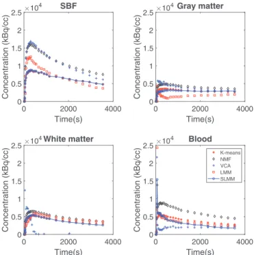
SBF 0 2000 4000 Time(s) 0 0.5 1 1.5 2 2.5 Concentration (kBq/cc) 104 White matter 0 2000 4000 Time(s) 0 0.5 1 1.5 2 2.5 Concentration (kBq/cc) 104 Gray matter 0 2000 4000 Time(s) 0 0.5 1 1.5 2 2.5 Concentration (kBq/cc) 104 Blood 0 2000 4000 Time(s) 0 0.5 1 1.5 2 2.5 Concentration (kBq/cc) 104 K-means NMF VCA LMM SLMM
Fig. 7. TACs obtained by estimation from the real image.
betterresults.Ontheother hand,itisalsotheaccurate initializa-tion provided byK-means forthe whitematter that allows LMM and SLMM to present good results for thisfactor in comparison with the other algorithms. BothVCA and NMF show a very low performance forthisfactorTAC,inoppositionto itsgood estima-tionofthegraymatterTAC.AsthegrayandwhitematterTACsare highlycorrelated,itisnaturaltoexpectambiguityontheirresults andtherefore,agoodperformance ononeofthemmaylowerthe performanceontheother.Concerningthebloodfactor,bothLMM and SLMM are able to overcome the poor K-means initialization andshowaveryaccurate performance,alongwithVCAandNMF. Inrealdata,whileVCAiscompletelyunabletodifferentiatetissues andLMMgetsfarawayfromtheK-meansinitialization,bothNMF andSLMMmaintaintheinitializationstructureforthenon-specific bindingtissues withsomeadditionalartifactsontheSLMMresult duetodeconvolution,asseeninFig.6.
Concerning high-uptake tissues, SLMM performs better than LMM andall the other algorithms forboth theSBFand its asso-ciatedproportion,asseeninFig.3,showingtheinterestof explic-itlymodelingthevariability.Indeed,thevariabilityproportionmap computed by SLMM, depicted inFig. 5 forsynthetic simulations, not onlydelineates thespecificbinding regionbutalsois ableto differentiatetheintensityofhigh-uptake.Thisaccurateestimation canbeexpectedtocharacterizetissuesdifferentlyaffectedbya tu-mor(someinearlystagesofmetastasisandothersalready aggres-sively affected) or, in the case of stroke, to detect regions more orlessaffectedbylackofoxygenorinflammation.When inspect-ingtheexperimentalresultsobtainedontherealdatasetinFig.8, the factor proportionrelated to specific binding seems to be es-timated witha visually higher precision by the proposed model thantheothers.SLMMprovidessharperandmoreaccuratemaps, characterized by a larger area with high uptake, as in the MRI ground-truth. Theproposedtechniqueseems todetectthis metic-ulousdifferences,whichareuntilnowneglectedinstate-of-the-art computer-aidedPETanalysis.
6.2. Flexibilityofthemethod
The method isan unsupervised approach andis easily adapt-abletoothercontexts.Inthiswork,tworadiotracersformicroglial
Stroke
0
0.5
1
Kmeans
0
0.5
1
NMF
0
0.5
1
VCA
0
0.5
1
LMM
0
0.5
1
SLMM
0
0.5
1
Variability
0
0.5
0
0.5
1
0
0.5
1
0
0.5
1
0
0.5
1
0
0.5
1
0
0.5
1
0
0.5
0
0.5
1
0
0.5
1
0
0.5
1
0
0.5
1
0
0.5
1
0
0.5
1
0
0.5
Fig. 8. From top to bottom: MRI ground-truth of the stroke area, SBF coefficient maps estimated by K-means, NMF, VCA, LMM, SLMM and SBF variability estimated by SLMM.
activation were studied.Syntheticimageswere based ona phan-tomthatpresentedthekineticsofthe[11C]-PE2Iradioligand,while real images were acquired from [18F]DPA-714 injection. Besides these two tracers, the algorithm may be adapted to any tracer andanysubjectinstudy.Tobetransposedtoanothersetting,the methodonlyrequires:
(a) asinallfactoranalysistechniques,thenumberofexpected kineticclassesinaROI;
(b) aninitialguessofthefactorsandproportions;
(c) a dictionary with the specific binding variability pattern, thatcanbelearnedaslongasTACscontainingspecific bind-ingkineticscanbeidentified.
Thus, changes in perfusion along patients and scans do not affect theperformance of themethod, since both(b) and(c)are subjectandscan-dependent,i.e.,areprovidedforeachsubjectand scan.Whatindeedaffectstheperformanceofthemethodisrather the quality of (b)and (c)previous estimations. In thiswork, the initial guess (b) was provided by K-means, however, the choice of the initialization can be adapted to the available data (e.g. a MRI scan of each subject, pre-defined population-based classes or atlas-based segmentations, SVCA results). The specific binding TACsneededin(c)wereidentifiedbyvisualinspectionforthereal
image, aprocedurethat cangenerallyberepeated inanycase, as longassomehigh-uptakevoxelscanbeidentified.Athresholding can also be used to identify theseTACs, e.g., the 10% maximum AUCvoxelsinthelastframes,orsomeatlasifhighspecificbinding regionsareknown,e.g.thethalamusfor[18F]DPA-714.
Note howeverthatwe alsohavea highnumberofpriorsthat mayneedto beadapted toeachnewscenario,eventhough their
a priori assumptionsare oftenverygeneric.The factorproportion penalization,relatedtothehomogeneityofneighboringregionsin the image, is a quite general prior forall biomedicalimage pro-cessing applications. The factors prior is relatedto the reliability ofinitialization. Itfurtherintensifiesthedependency oftheLMM and SLMM solutions on a good initialization of factors but also allows to benefit from a previous knowledge on the pattern of the factors,e.g.,thekineticsofthetracer.Finally,theprior ofthe variabilityrelatedtospecificbindinginducessparsity,i.e.,assumes thatonlyafewvoxelsintheimageareimpactedbyspecific bind-ing. The [11C]-PE2I is expectedto mainly specificallybind inthe striatum, so,in thiscase, sparsity isan adequate assumption.On theother hand,the[18F]DPA-714targetsmicroglialactivationand thereforeneuroinflammationinthebrain,whichcanpotentially af-fect a greaterpart oftheimage, inoppositionto thesparsity as-sumption.Nevertheless,inourspecificcaseofstrokepatients, neu-roinflammation was mainly expected in the stroke area and the thalamuswhichrepresentaverysmallpartofthebrain,therefore thisassumptionwas stilladequate. Dependingontheapplication, the intensityofthe expectedsparsity maybeeasily regulated by its corresponding weight (as for the other penalties), i.e., if spe-cificbindingisexpectedinagreaterpartoftheimage,wemay re-ducethelevelofthesparsitypenaltyorevensetittozero.Soitis alsoquiteadaptable.However,thishighlightsadrawbackfromour method thatisthehighnumberofhyperparametersto betuned. The use ofautomatic estimationstrategies within the algorithms shouldbeenvisagedinfuturedevelopments.
7. Conclusionandfutureworks
This paper introduced a new model to conduct factor analy-sis ofdynamic PETimages.Itreliedon theunmixingconcept ac-countingforspecificbindingTACsvariation.Themethodwasbased on the hypothesis that the variations within the SBF can be de-scribedbyasmallnumberofbasiselementsandtheir correspond-ing proportions per voxel. The resulting optimization problemis extremely non-convexwithhighlycorrelatedfactorsand variabil-itybasiselements,whichleadstoahighnumberofspuriouslocal optimaforthecostfunction.However,theexperimentsconducted onsyntheticdatashowedthattheproposedmethodsucceededin estimating thisvariability, which improved the estimation ofthe specific bindingfactorandthecorresponding proportions.Forthe other quantitiesof interest, theproposed approachcompared fa-vorably withstate-of-the-art unmixing techniques. The proposed approach has manypotential applications in dynamic PET imag-ing. Itcould beused forthe segmentationofa region-of-interest, classificationofthevoxels,creationofsubject-specifickinetic refer-enceregionsorevensimultaneousfilteringandpartialvolume cor-rection.Besidesexploring suchapplications ofthe method,future works should focuson theintroduction ofa Poisson-fitting mea-sureofdivergenceused inthecostfunction, e.g.Kullback-Leibler, tobettermodelnoisefrequentlyencounteredinlowratePETdata.
References
Bai, B., Bading, J., Conti, P.S., 2013. Tumor quantification in clinical positron emission tomography. Theranostics 3 (10), 787–801. doi: 10.7150/thno.5629 .
Barber, D.C. , 1980. The use of principal components in the quantitative analysis of gamma camera dynamic studies. Phys. Med. Biol. 25 (2), 283–292 .
Bioucas-Dias, J.M. , Figueiredo, M.A.T. , 2010. Alternating direction algorithms for con- strained sparse regression: Application to hyperspectral unmixing. In: Proceed- ings of the IEEE GRSS Workshop Hyperspectral Image SIgnal Process.: Evolution in Remote Sens. (WHISPERS) .
Bioucas-Dias, J.M., Plaza, A., Dobigeon, N., Parente, M., Du, Q., Gader, P., Chanus- sot, J., 2012. Hyperspectral unmixing overview: geometrical, statistical, and sparse regression-based approaches. IEEE J. Sel. Topics Appl. Earth Observ. Re- mote Sens. 5 (2), 354–379. doi: 10.1109/jstars.2012.2194696 .
Boellaard, R., Turkheimer, F.E., Hinz, R., Schuitemaker, A., Scheltens, P., van Berckel, B.N.M., Lammertsma, A .A ., 2008. Performance of a modified super- vised cluster algorithm for extracting reference region input functions from (r)- [11c]pk11195 brain pet studies. In: Proceedings of the 2008 IEEE Nuclear Sci- ence Symposium Conference Record, pp. 5400–5402. doi: 10.1109/NSSMIC.2008. 4774453 .
Bolte, J., Sabach, S., Teboulle, M., 2013. Proximal alternating linearized minimization for nonconvex and nonsmooth problems. Math. Program. 146 (1–2), 459–494. doi: 10.1007/s10107- 013- 0701- 9 .
Bullmore, E., Long, C., Suckling, J., Fadili, J., Calvert, G., Zelaya, F., Carpenter, T.A., Brammer, M., 2001. Colored noise and computational inference in neurophysi- ological (fMRI) time series analysis: resampling methods in time and wavelet domains. Hum. Brain Mapp. 12, 61–78. doi: 10.1109/tns.2003.817963 .
Cavailloles, F. , Bazin, J.P. , Di Paola, R. , 1984. Factor analysis in gated cardiac studies. J. Nuclear Med. 25, 10671079 .
Cavalcanti, Y.C. , Oberlin, T. , Dobigeon, N. , Stute, S. , Ribeiro, M. , Tauber, C. , 2017. Un- mixing dynamic PET images with variable specific binding kinetics – Supporting materials. Technical Report. University of Toulouse, IRIT/INP-ENSEEIHT, France .
Chou, Y.-C., Teng, M.M.H., Guo, W.-Y., Hsieh, J.-C., Wu, Y.-T., 2007. Classification of hemodynamics from dynamic-susceptibility-contrast magnetic resonance (dsc- mr) brain images using noiseless independent factor analysis. Med. Image Anal. 11 (3), 242–253 . 10.1016/j.media.20 07.02.0 02.
Condat, L., 2015. Fast projection onto the simplex and the l 1 -ball. Math. Program.
158 (1–2), 575–585. doi: 10.1007/s10107- 015- 0946- 6 .
Dobigeon, N. , Brun, N. , 2012. Spectral mixture analysis of EELS spectrum-images. Ultramicroscopy 120, 25–34 .
El Fakhri, G. , Sitek, A. , Gurin, B. , Kijewski, M.F. , Di Carli, M.F. , Moore, S.C. , 2005. Quantitative dynamic cardiac 82 r b PET using generalized factor and compart- ment analyses. J. Nuclear Med. 46 (8), 1264–1271 .
Fessler, J.A. , 1994. Penalized weighted least-squares image reconstruction for positron emission tomography. IEEE Trans. Med. Imag. 13 (2), 290–300 . Gunn, R.N. , Lammertsma, A .A . , Hume, S.P. , Cunningham, V.J. , 1997. Parametric imag-
ing of ligand-receptor binding in PET using a simplified reference region model. Neuroimage 6, 279–287 .
Häggström, I. , Beattie, B.J. , Schmidtlein, C.R. , 2016. Dynamic PET simulator via tomo- graphic emission projection for kinetic modeling and parametric image studies. Med Phys 43 (6), 3104–3116 . Part 1.
Halimi, A., Dobigeon, N., Tourneret, J.-Y., 2015. Unsupervised unmixing of hyperspec- tral images accounting for endmember variability. IEEE Trans. Image Process. 24 (12), 4 904–4 917. doi: 10.1109/tip.2015.2471182 .
Henrot, S. , Soussen, C. , Dossot, M. , Brie, D. , 2014. Does deblurring improve ge- ometrical hyperspectral unmixing? IEEE Trans. Image Process. 23 (3), 1169– 1180 .
Huang, Y. , Zaas, A.K. , Rao, A. , Dobigeon, N. , PETer J. Woolf , Veldman, T. , Oien, N.C. , McClain, M.T. , Varkey, J.B. , Nicholson, B. , Carin, L. , Kingsmore, S. , Woods, C.W. , Ginsburg, G.S. , Hero, A. , 2011. Temporal dynamics of host molecular responses differentiate sym ptomatic and asymptomatic influenza a infection. PLoS Genet. 8 (7) .
Innis, R.B., Cunningham, V.J., Delforge, J., Fujita, M., Gjedde, A., Gunn, R.N., Holden, J., Houle, S., Huang, S.-C., Ichise, M., et al., 2007. Consensus nomenclature for in vivo imaging of reversibly binding radioligands. J. Cereb. Blood Flow Metab 27 (9), 1533–1539. doi: 10.1038/sj.jcbfm.9600493 .
Keshava, N. , 2003. A survey of spectral unmixing algorithms. Lincoln Lab. J. 14, 56–78 .
Lee, D.D. , Seung, H.S. , 20 0 0. Algorithms for non-negative matrix factorization. In: Proceedings of the Neural Information Processing System .
Lee, J.S. , Lee, D.D. , Choi, S. , Park, K.S. , Lee, D.S. , 2001. Non-negative matrix factoriza- tion of dynamic images in nuclear medicine. In: Proceedings of the IEEE Nuclear Science Symposium (NSS) .
Martel, A.L., Moody, A.R., Allder, S.J., Delay, G.S., Morgan, P.S., 2001. Extracting para- metric images from dynamic contrast-enhanced MRI studies of the brain us- ing factor analysis. Med. Image Anal 5 (1), 29–39. doi: 10.1016/S1361-8415(00) 0 0 032-3 .
Mehranian, A. , Belzunce, M.A. , Niccolini, F. , Politis, M. , Prieto, C. , Turkheimer, F. , Hammers, A. , Reader, A.J. , 2017. PET Image reconstruction using multi-paramet- ric anato-functional priors. Phys. Med. Biol. 62 (15), 5975 .
Muzi, M. , Mankoff, D.A. , Grierson, J.R. , Wells, J.M. , Vesselle, H. , Krohn, K.A. , 2005. Ki- netic modeling of 3-deoxy-3-fluorothymidine in somatic tumors: mathematical studies. J. Nuclear Med. 46 (2), 371–380 .
Nascimento, J., Dias, J., 2005. Vertex component analysis: a fast algorithm to unmix hyperspectral data. IEEE Trans. Geosci. Remote Sens. 43 (4), 898–910. doi: 10. 1109/tgrs.2005.844293 .
Padilla, P., Lpez, M. , Grriz, J.M. , Ramrez, J. , Salas-Gonzlez, D. , lvarez, I. , 2012. NM- F-SVM based cad tool applied to functional brain images for the diagnosis of Alzheimers disease. IEEE Trans. Med. Imag. 31, 207–216 .
Park, S.-U. , Dobigeon, N. , Hero, A.O. , 2014. Variational semi-blind sparse deconvolu- tion with orthogonal kernel bases and its application to MRFM. Signal Process. 94, 386–400 .
Phelps, M.E. , Mazziotta, J.C. , Schelbert, H.R. , 1986. Positron Emission Tomography and Autoradiography (Principles and Applications for the Brain and Heart). Raven, New York .
Rahmim, A. , Qi, J. , Sossi, V. , 2013. Resolution modeling in PET imaging: theory, prac- tice, benefits, and pitfalls. Med. Phys. 40 (6) .
Schiepers, C., Chen, W., Dahlbom, M., Cloughesy, T., Hoh, C.K., Huang, S.-C., 2007. 18F-fluorothymidine kinetics of malignant brain tumors. Eur. J. Nuclear Med. Molecular Imag. 34 (7), 1003–1011. doi: 10.1007/s00259- 006- 0354- 5 .
Schulz, D., 2013. Non-negative matrix factorization based input function extraction for mouse imaging in small animal PET - comparison with arterial blood sam- pling and factor analysis. J. Molecular Imag. Dyn. 02. doi: 10.4172/2155-9937. 10 0 0108 .
Shepp, L. , Vardi, Y. , 1982. Maximum likelihood reconstruction for emission tomog- raphy. IEEE Trans. Med. Imag. 113–122 .
Sitek, A. , Di Bella, E.V.R. , Gullberg, G.T. , 20 0 0. Factor analysis with a priori knowl- edge - application in dynamic cardiac SPECT. Phys. Med. Biol. 45, 2619–2638 . Sitek, A. , Gullberg, G.T. , Huesman, R.H. , 2002. Correction for ambiguous solutions in
factor analysis using a penalized least squares objective. IEEE Trans. Med. Imag. 21 (3), 216225 .
Stute, S. , Tauber, C. , Leroy, C. , Bottlaender, M. , Brulon, V. , Comtat, C. , 2015. Analyt- ical simulations of dynamic PET scans with realistic count rates properties. In: Proceedings of the IEEE Nuclear Science Symposium on Medical Imaging Con- ference (NSS-MIC) .
Thireou, T. , Pavlopoulos, S. , Kontaxakis, G. , Santos, A. , 2006. Blind source separation for the computational analysis of dynamic oncological PET studies. Oncol. Rep. 15, 10071012 .
Thouvenin, P.-A. , Dobigeon, N. , Tourneret, J.-Y. , 2016. Hyperspectral unmixing with spectral variability using a perturbed linear mixing model. IEEE Trans. Signal Process. 64 (2), 525–538 .
Tibshrani, R. , 1996. Regression shrinkage and selection via the lasso. J. Roy. Stat. Soc. 58 (1), 267–288 .
Tichý, O. , Šmídl, V. , 2015. Bayesian Blind Separation and Deconvolution of Dynamic Image Sequences Using Sparsity Priors. IEEE Trans. Med. Imag 34 (1), 258–266 .
Turkheimer, F., Aston, J., Banati, R., Riddell, C., Cunningham, V., 2003. A linear wavelet filter for parametric imaging with dynamic PET. IEEE Trans. Med. Imag. 22 (3), 289–301. doi: 10.1109/tmi.2003.809597 .
Wilson, D. , Tsui, B. , Barrett, H. , 1994. Noise properties of the EM algorithm. II. monte carlo simulations. Phys. Med. Biol. 39, 847–871 .
Winter, M.E. , 1999. N-FINDR: an algorithm for fast autonomous spectral end-mem- ber determination in hyperspectral data. In: Descour, M.R., Shen, S.S. (Eds.), Pro- ceedings of the SPIE Imaging Spectrometry V. SPIE, pp. 266–275 .
Wu, H.-M. , Hoh, C.K. , Choi, Y. , Schelbert, H.R. , Hawkins, R.A. , Phelps, M.E. , Huang, S.-C. , 1995. Factor analysis for extraction of blood time-activity curves in dynamic FDG-PET studies. J. Nuclear Med. 36 (9), 1714–1722 .
Yaqub, M., van Berckel, B.N., Schuitemaker, A., Hinz, R., Turkheimer, F.E., Tomasi, G., Lammertsma, A .A ., Boellaard, R., 2012. Optimization of supervised cluster anal- ysis for extracting reference tissue input curves in (r)-[11C]pk11195 brain PET studies. J. Cereb. Blood Flow Metab. 32 (8), 1600–1608. doi: 10.1038/jcbfm.2012. 59 .
Zare, A., Ho, K., 2014. Endmember variability in hyperspectral analysis: addressing spectral variability during spectral unmixing. IEEE Signal Process. Mag. 31 (1), 95–104. doi: 10.1109/msp.2013.2279177 .