Any correspondence concerning this service should be sent to the repository
administrator:
staff-oatao@listes-diff.inp-toulouse.fr
O
pen
A
rchive
T
OULOUSE
A
rchive
O
uverte (
OATAO
)
OATAO is an open access repository that collects the work of Toulouse researchers and
makes it freely available over the web where possible.
This is an author-deposited version published in:
http://oatao.univ-toulouse.fr/
Eprints ID: 15988
To cite this version:
Masmoudi, Malek and Hans, Erwin W. and Haït, Alain Tactical
project planning under uncertainty: fuzzy approach. (2016) European Journal of Industrial
Engineering, vol. 10 (n° 3). pp. 301-317. ISSN 1751-5254
Official URL:
http://dx.doi.org/10.1504/EJIE.2016.076381
Tactical project planning under uncertainty: Fuzzy approach
Abstract
At the tactical planning level in a multi-project environment, uncertainties are inherent to the workloads of the activities, and costs may be involved for using non-regular capacity and for violating project due dates. Examples of such environments are found in engineer-to-order environments like construction, and ship yards. We offer in this paper an approach that allows project management to identify per period whether non-regular capacities (overtime, hiring and subcontracting) might be needed to meet the projects’ negotiated due dates. The studied problem is known as the Rough Cut Capacity Planning problem (RCCP) under uncertainty. We propose a possibilistic approach, which is based on modeling uncertain workloads with fuzzy sets. We present the resulting Fuzzy Rough Cut Capacity Planning (FRCCP problem), and show that we can use the possibilistic approach to provide a robust solution with a fuzzy resource loading profile that serves as a decision support for the managers. To solve the FRCCP problem, we provide a Simulated Annealing metaheuristic. We test it against several of the existing RCCP approaches. For the experiments we use real life instances from a shipyard maintenance center.
Keywords: project planning, RCCP, uncertainty, workload, fuzzy sets, possibilistic approach, simulated annealing.
1. Introduction
Multi-project organizations face decision problems on project acceptance, resource allocation, coordi-nation, etc., with multiple (internal or external) customers. This context demands a structured planning process [8]. At the tactical planning level, Rough-Cut Capacity Planning (RCCP) is applied during the ne-gotiation stage with a customer [19]. It consists of studying the impact of project acceptance on the resource capacity usage and provides a feasible and competitive project delivery date. At this level, a project is viewed as a set of macro-tasks with both precedence and resource constraints. A macro-task may require specific skills to be completed (e.g., mechanical skills). Costs are incurred when nonregular capacity (e.g., overtime, hiring, subcontracting) is used, or when project due dates are not met. Rough-cut capacity planning aims at allocating the appropriate workforce, on a periodic basis, in order to complete the macro-tasks within their time windows at a minimum cost. The deterministic RCCP problem is NP-hard [23, 36]. Integrating uncertainties increases the problem complexity [46, 47].
Planning the activity of large Dutch ship repair yard at the tactical level is considered as an application of the Rough-Cut Capacity Planning (RCCP) [8, 46] where uncertainty is particularly present. The reparation of a ship is considered as a project and several ships are repaired at the same time. The shipowner and the shipyard negotiate the details of the project: the starting time (receiving date), the list of macro-tasks, the costs, and the finishing time (delivery date). The shipyard must make a realistic offer before having seen the damage on the ship [46]. The project execution is not free from uncertainty and unexpected events, e.g., the starting time may be delayed, additional work may appear after the first inspection, and required resources may be unavailable.
Two approaches can be considered simultaneously or separately to solve the tactical planning problem: the time-driven approach and the resource-driven approach. The former aims to minimize overcapacity cost (overtime, hiring and subcontracting capacity cost) given fixed due dates, and the latter aims to minimize the costs incurred by projects’ lateness given fixed capacity levels. In this paper we adopt the time-driven approach, which is, in our experience, the most common approach in practice. To deal with uncertainty, we will introduce a robustness criterion. This concept, which is also called stability, has gained the interest of
several researchers in operational [25] and tactical planning [47]. Hans [19] has proposed a branch-and-price technique to solve the deterministic RCCP. Wullink et al. [47] have extended Hans’ deterministic model to a scenario-based approach based on a discretization of the stochastic work content. They consider a time-driven problem and also introduce different robustness objective functions.
In this paper, we consider fuzzy numbers to model uncertainty on work contents and propose a simulated annealing algorithm to solve the RCCP problem under uncertainty. Planning the activity of a Dutch ship repair yard is considered as an application in our study and benchmark instances from [46] are considered for computations.
Section 2 contains the RCCP problem statement. Section 3 outlines fuzzy sets as one of the modeling approach for dealing with uncertainty in comparison to the most used approach, which is the stochastic approach. Section 4 contains a generalization of the RCCP problem to a fuzzy version. Section 5 describes a Simulated Annealing (SA) algorithm to solve the Fuzzy RCCP variant. In section 6, the SA algorithm is applied to real-life instances and validated in comparison to existing algorithms. Section 7 contains the conclusions.
2. RCCP problem statement and linear programming
To introduce the RCCP problem we consider the exact MILP formulation proposed by [19] that we generalized to accommodate uncertainty. We consider a set N of projects, each composed of tasks (b, j), j ∈ N , b ∈ Nj. A project is constrained by its release date and deadline, and so are its macro-tasks; precedence constraints also applied between different macro-tasks of one project. The work content of macro-task (b, j) is uncertain and denoted by ˜pbj and its minimum duration is ωbj. The minimum durations are a result of technical constraints such as available working space and expected precedence relations between activities at a lower level.
To perform a macro-task, several skills may be needed. A resource group i ∈ I is associated to each skill. The fraction of macro-task work content ˜pbj to be performed by resource group i is written as υbji, with P
i∈Iυbji= 1 for all b, j. The planning horizon consists of T periods. Decision variables Ybjt represent the fraction of the work content of macro-task (b, j) executed in period t.
We consider Πjthe set of all feasible project plans for project j. A project plan ajπ∈ Πjfor project j is a vector of 0-1 values abjtπ (b ∈ Nj; t = 1, . . . , T ), where abjtπ = 1 if task (b, j) is allowed to be performed in period t, 0 otherwise. Binary variable Xjπ takes value 1 if project plan ajπ is selected for project j, 0 otherwise.
A complete mathematical model for the RCCP is formulated as follows (the parameters and variables that we consider ”uncertain” in the next section are shown with a tilde: “∼”):
minimize I X i=1 T X t=0
subject to X π∈Πj Xjπ= 1, j ∈ N (2) Ybjt− 1 ωbj X π∈Πj abjtπXjπ≤ 0, j ∈ N ; b ∈ Nj; t = 1, .., T (3) T X t=1 Ybjt = 1 j ∈ N ; b ∈ Nj (4) X j∈N X b∈Nj ˜
pbjυbjiYbjt≤ κi1t+ ˜Oit+ ˜Hit+ ˜Sit, i ∈ I; t = 1, .., T (5) ˜
Oit≤ κi2t− κi1t, i ∈ I; t = 1, .., T (6)
˜
Hit≤ κi3t− κi2t, i ∈ I; t = 1, .., T (7)
˜
Oit, ˜Hit, ˜Sit≥ 0, i ∈ I; t = 1, .., T (8)
Xjπ∈ {0, 1}, j ∈ N ; π ∈ Πj (9)
Ybjt∈ [0, 1], j ∈ N ; b ∈ Nj; t = 1, .., T (10)
In this formulation, κi1tis the regular capacity available of resource i in period t, κi2tis the sum of regular and overtime capacity, and κi3t equals κi2t augmented with the capacity available by hiring non-regular temporary (interim) staff. Variable ˜Oit is the uncertain number of overtime hours of resource i in period t, ˜Hit is the uncertain number of hours performed by interim workers and ˜Sit is the uncertain number of subcontracted hours. The constants ςi1, ςi2and ςi3specify the costs of using one hour of non-regular capacity (overtime ˜Oit, hiring ˜Hit, and subcontracting ˜Sit, respectively).
The objective function (1) is a linear function that minimizes the uncertain cost of non-regular capacity; overtime is less expensive than interim work, which in turn is cheaper than subcontracting. The concept of project plans stems from [19]; project plans can incorporate calendar constraints (time windows) and precedence constraints. Constraints (2) ensure that exactly one project plan is selected for each project. Constraints (3) specify a minimum duration ωbj for macro-task (b, j) and impose consistency of the project schedule (the Y -variables) with the project plan. Constraints (4) guarantee that all work is done. Finally, Equations (5)–(7) are the capacity constraints.
The described RCCP incorporates ready times and deadlines (in the project plans) and is NP-hard. Since the number of project plans to be considered grows exponentially with the size of N and Nj, Hans [19] uses branch-and-price to find an optimal integer solution and Gademann and Schutten [15] uses several LP-based heuristics for a better computation time.
3. Uncertainty modeling
The scientific study of uncertainty probably started in 1654 by Pascal and Fermat with the development of probability theory [41]. Formally, it is well known that if X is a continuous random variable within an uncountable domain S, then it has a probability density function p(x), and therefore its probability to fall into a given interval, say [A, B], is given by the integral Pr[A ≤ X ≤ B] =RB
A p(x)dx. Hence, the probability distribution is completely characterized by its cumulative distribution function F (x). This latter gives the probability that the random variable is not larger than a given value F (x) = Pr [X ≤ x] ∀x ∈ S.
The study of imprecision and subjective uncertainty came far later in 1965 when Zadeh [48] proposed the fuzzy set theory. This new theory is a generalization of classical set theory. It is based on the idea that vague notions without clear limits such as “old”, “near”, “short” can be modeled by a gradual number called “fuzzy subset”. The representation of vagueness and imprecision became consequently possible thanks to fuzzy logic. Possibility theory was then developed by Zadeh [49] as alternative to probability theory for
dealing with a non-probabilistic uncertainty that is modeled with fuzzy logic. This new theory treats uncertainty and imprecision with the same formalism.
A fuzzy set eA is mathematically defined as a subset of a referential set X, whose boundaries are gradual rather than abrupt. A fuzzy number eA is a convex and normal fuzzy set. It refers to a connected set of possible values called degree of membership (µ
e
A(x), x ∈ X) taking values in [0, 1]. These possible values form a profile called the membership function µ
e
A. Many types of profiles are used in literature to represent fuzzy numbers e.g 6-point, 4-point and 3-point linear membership possibilities (see Figure 1). Particularly, the trapezoidal profile (4-point) is well-supported by the possibility approach [10]. It is the one that we consider in this paper because it is the most appropriate to our case of study.
µ e A(x) 1 x aA bA cA dA µ e A(x) 1 x aA bA cA dA eA fA µ e A(x) 1 x aA bA dA
Figure 1: Frequently used profiles: 6-point, 4-point and 3-point linear membership functions
A trapezoidal fuzzy number eA is represented by a 4-tuple (i.e., eA = (aA, bA, cA, dA)). The first and fourth elements (aA and dA) correspond to the extremes from where the membership function begins to grow, and the second and third elements (bAand cA) define the interval that limits the maximum degree of membership (generally considered equal to 1).
Dubois and Prade [10], and Chen and Hwang [6] have defined mathematical operations that can be performed on trapezoidal fuzzy sets. Let eA(aA, bA, cA, dA) and eB(aB, bB, cB, dB) be two independent trape-zoidal fuzzy numbers, then:
e
A ⊕ eB = (aA+ aB, bA+ bB, cA+ cB, dA+ dB) (11) α eA =
(
(αaA, αbA, αcA, αdA) if α > 0
(αdA, αcA, αbA, αaA) if α ≤ 0 (12)
Other operations like subtraction, multiplication, division, intersection and union have also been studied. For more details regarding fuzzy arithmetic, we refer readers to [4, 10].
The possibility theory was introduced by [49] to provide a mean to take into account the uncertainties. It is based on fuzzy subsets and introduces both a possibility measure (denoted Π) and a necessity measure (denoted N ).
Let P to be a crisp number, and eA is a fuzzy number attached to a single valued variable x. The possibility (necessity) of the event ”x ≤ P ”, denoted by Π(x ≤ P ) (N (x ≤ P )), evaluates the extent to which the event is ”possibly true” (”necessarily true”). It is defined as the degree of intersection between eA and ] − ∞, P ] by the following operations:
Π( eA ≤ P ) = sup u min(µ e A(u), µ(−∞,P [(u)) = sup u≤P µ e A(u) (13) N ( eA ≤ P ) = 1 − Π( eA > P ) = 1 − sup u>P µ e A(u) = inf u>P(1 − µAe(u)) (14)
Many papers in literature compare fuzzy/possibilistic to other approaches dealing with uncertainty mod-eling [11, 21, 31, 35, 40]. Kosko [24] claims that probability theory is a sub-theory of fuzzy logic. Zadeh [50],
the creator of fuzzy logic and the so-called possibilistic approach, claims that probability theory and fuzzy logic are complementary rather than competitive and that possibility theory is the alternative to probability. Fuzzy modeling is used when little and imprecise information is available [1, 7]. It is often judged appro-priate to represent subjective uncertainty and full or partial ignorance. Based on fuzzy set modeling, possi-bility theory offers a framework to model implicit information given by experts. Fuzzy arithmetics are easy to manipulate whatever the complexity of the considered profile, and this fact makes the fuzzy/possibilistic approach powerful enough to attract the attention of many authors in different research domains, and par-ticularly in planning and scheduling [3, 26, 28, 29, 33, 44, 45]. Today, fuzzy scheduling and planning is a specific field for several journals e.g Fuzzy Optimization and Decision Making.
In this article, we consider fuzzy sets distributions to deal with uncertainty modeling. The uncertain parameters and variables in the MILP model provided in Section 2 are modeled with fuzzy sets. We refer to this problem as Fuzzy RCCP (FRCCP).
4. Fuzzy RCCP
Uncertainty in tactical planning is present in macro-task work contents [12, 20]. Macro-tasks work contents can be established by asking experts. In the fuzzy planning literature, the operational (scheduling) level of planning has received the most attention [16, 3, 26, 29], and tactical planning has remained rather underexposed [13, 18, 42, 44]. To the best of our knowledge, Masmoudi et al. [30] is the first reference to deal with the fuzzy tactical project planning.
In this work, we consider 4-point fuzzy numbers called trapezoidal profile. Each macro-task work content is divided into portions that are allocated to the time periods between the macro-task’s starting and finishing dates [30].
Let us consider an example of macro-task A with a fuzzy work contentpeA= (120, 180, 240, 300), present from period 3 to period 5; here and throughout the text, a tilde ”∼” over a quantity indicates that the quantity is a fuzzy number. Let us suppose that one third of the work content is to be executed by resource type 1 (υA1 = 1/3) and two thirds correspond to resource type 2 (υA2 = 2/3). We choose to carry out three quarters of the macro-task A at period 3 (YA3= 3/4) and the other quarter at period 4 (YA4= 1/4). Table 1 shows the macro-task and its different work content portions.
Table 1: Fuzzy macro-task resource portions
Macro-task Resource type Period 3 Period 4
A 1 (30,45,60,75) (10,15,20,25)
A 2 (60,90,120,150) (20,30,40,50)
The workload fWit on resource i in period t is calculated as fWit = Pb,jpebjυbjiYbjt. fWit is calculated using simple fuzzy mathematical operations (addition and multiplication) as defined in [10, 6].
Below we first look into evaluation of the costs (Section 4.1) and subsequently we discuss robustness functions (Section 4.2).
4.1. Fuzzy cost expectation
As in the deterministic case, the FRCCP aims at minimizing the total cost of non-regular capacity usage (overtime, hiring and subcontracting). In our case, the non-regular capacity usage is fuzzy because it represents the portion of the fuzzy workload between the different capacity limits. The objective function to minimize the costs of the use of non-regular capacity is:
minimize I X i=1 T X t=0
To transform a fuzzy quantity into a deterministic quantity, the defuzzification technique is one of the easiest ways that have been used in the literature [37]. In particular, a simple formula has been proposed for trapezoidal profiles [5, 9, 14, 34, 37]. Using this formula, we obtain the following cost expectation:
E = I X i=1 T X t=0 l X m=1
qm(ςi1Oitm+ ςi2Hitm+ ςi3Sitm) (16)
Hence, the cost expectation is a weighted sum of the costs for various work content values of fuzzy non-regular capacities (weights qm). Here, with trapezoidal fuzzy numbers, we have l = 4 values for each fuzzy number. These values are related to the risk that the managers take by giving more or less importance to the possibility and necessity profiles. According to Liu and Liu [27], we consider q1 = q2 = (1−β)2 , which corresponds to weights assigned to the extreme points of the possibility profile and q3= q4= β2, which are weights assigned to the extreme points of the necessity profile. β is considered greater than 12 to give more importance to the necessity profile.
4.2. Fuzzy robustness functions
Contrary to the tactical planning problem where uncertainty is mainly on macro-task workload, in the fuzzy scheduling problem the uncertainty is mainly on task duration and expected order due date. In the fuzzy scheduling literature, two approaches exist to calculate the robustness of a schedule to the lateness criterion: one based on the possibility measure and the other on intersection areas [6, 39]. Let us denote eCj the fuzzy completion time of project j and edjits due date, with µ
e
Cj and µdej their corresponding membership
functions. The two robustness functions, also called satisfaction grades (SG), are: SG1 = Π
e
Cj( edj) = supx min(µCej(x), µdej(x)) (17)
SG2 = area( eCj∩ edj)/area( eCj) (18)
While area( eCj) measures the surface area of the fuzzy number eCj and area( eCj∩ edj) measures the area of overlap between edj and eCj, .
For the FRCCP problem, we propose to measure the robustness as the ”necessity and possibility” of a workload plan to respect the capacity limits i.e. the difference between the fuzzy workload and the available capacity.
Let fWit be the fuzzy workload and κit be the capacity limit of resource i at period t = 0, . . . , T . To verify whether the fuzzy workload respects the capacity limit, we measure the truth of event fWit≤ κitusing the couple possibility (Π(fWit≤ κit)) and necessity (N (fWit≤ κit)). Thus:
Π(fWit≤ κit) = sup u≤κit
µ f
Wit(u) (19)
N (fWit≤ κit) = 1 − Π(κit< fWit)= inf u>κit
(1 − µ f
Wit(u)) (20)
Let Nitand Πitbe the values of the workload membership function intersection with the capacity limits: ∀i, t Nit= N (fWit≤ κit) and Πit= Π(fWit≤ κit) (∀i, t) with N and Π the possibility and necessity measures respectively. Let fWit= (Wit1, Wit2, Wit3, Wit4). Expressions Nit and Πitare calculated as follows:
Nit= 0 if κit< Wit3 κit−Wit3
Wit4−Wit3 if κit∈ [Wit3, Wit4]
1 if κit> Wit4 (21) Πit= 0 if κit< Wit1 κit−Wit1
Wit2−Wit1 if κit∈ [Wit1, Wit2]
1 if κit> Wit2
Fig. 2a presents the membership function of a fuzzy workload (µ f
Wit), its complementary (1 − µWfit)
and a real value (κit) varying from 0 to ∞ on the domain of the workload. Fig. 2b shows the possibility and necessity that the workload is inferior to κit. The possibility that the workload is lower than κit (Π(fWit≤ κit)), for κit varying from 0 to ∞ on the domain of the workload, is equal to 1 until κit reaches the last value u for which µ
f
Wit(u) = 1, then decreases according to the same slope than µfWit. The necessity
that the workload is lower than κit (N (fWit ≤ κit)), for κit varying from 0 to ∞ on the domain of the workload, is equal to 1 until κit reaches the decreasing slope of 1 − µ
f
Wit(u), then follows the slope until
1 − µ f
Wit(u) = 0.
This representation is similar to the one proposed by Grabot et al. [18] to model uncertainty in orders in MRP. Contrary to Grabot et al. [18] who measured the necessity and the possibility of the event ”fWit≥ κit”, we considered here the complementary event (fWit≤ κit) by respecting that N ( eA ≤ P )= 1 − Π( eA > P ).
Fig. 2c shows the way to represent a fuzzy load by period using the necessity and possibility measures using a rotation. The result is close to the bar graphs usually used for a workload planning visualization, but contains two inclined lines representing the possibility and the necessity profiles, instead of only one horizontal line. 1 Wit1 Wit2 Wit3 Wit4 µ f Wit 1 − µWitf κit u 1 Wit1 Wit2 Wit3 Wit4 Π(fWit≤ κit) N (fWit≤ κit) u u 1 0 Wit1 Wit2 Π(fWit≤ κit) Wit3 Wit4 N (fWit≤ κit)
2a. Fuzzy work content 2b. Possibility/Necessity 2c. Fuzzy workload
Figure 2: How to get a fuzzy load by period using the necessity and possibility measures
For the FRCCP problem, it is necessary to compare fuzzy workloads to the three deterministic capacity limits: regular, overtime and hiring, respectively denoted κi1t, κi2t, κi3t.
Inspired by SG1 (17), a first robustness expression is provided, based on possibility and necessity mea-sures: R1= PT t=0 PI i=1 P3 p=1ςip(βNipt+ (1 − β)Πipt) (T + 1)(PIi=1P3p=1ςip) (23)
The weighted sum βNipt+ (1 − β)Πipt expresses the credibility of fWit being under the limit κipt. Liu and Liu [27] proposed to set β to 1/2 but it is possible to consider other expressions of the credibility by giving to β other values in [0, 1].
Inspired by SG2 (18), a second fuzzy robustness function is provided, based on intersection area:
R2= PT t=0 PI i=1 P3 p=1ςip( β Sipt+1 + 1−β S0 ipt+1) (T + 1)(PKi=1P3p=1ςip) (24) This function accounts for the necessary and potential excess value of workload over the capacity limit, represented by surfaces Sipt and Sipt0 , whereas the previous one relies on necessity and possibility of excess. Figure 3 shows the robustness coefficients Nipt, Πipt, Sipt and Sipt0 .
The fuzzy workload fWit at period t is equal toP
bjYbjtυbjipbj. The areas Sipt˜ and S 0
ipt are determined as shown in Figure 4.
f Wit 0 1 Si3t Ni3t 0 1 f Wit Si2t Si2t0 Πi2t f Wit 0 1 Si1t Si1t0
Πi1t Regular capacity
Overtime Hired capacity Subcontracted capacity κi1t κi2t κi3t Wit1 Wit2 Wit3 Wit4
Figure 3: Fuzzy distribution and robustness coefficients
for t = 0 to T , i = 1 to I, p = 1 to 3 do if Wit4< κipt then
Sipt= 0
else if Wit3> κipt or Wit3= Wit4 then Sipt= Wit3+Wit4
2 − κipt else Sipt= (Wit4−κipt)2 2(Wit4−Wit3) end if
if Wit2< κipt then Sipt0 = 0
else if Wit1> κipt or Wit1= Wit2then Sipt0 = Wit1+Wit2
2 − κipt else
Sipt0 = (Wit2−κipt)2
2(Wit2−Wit1)
end if end for
Figure 4: Pseudo-code for determining the areas Siptand Sipt0
We mention that the robustness function R1 reflects a more optimistic attitude to overcapacity than the robustness function R2. In fact, R2 considers the highest point of intersection of the two fuzzy sets regardless of their overall dimensions, while R1 considers the proportion of the fuzzy workload that falls within the deterministic capacity limits (inspired by [32, 38]).
The mixed-integer linear programming (MILP) model for the FRCCP is formulated as follows (fuzzy parameters are defuzzified):
minimize I X i=1 T X t=0 ((1 − β)
2 [ςi1(Oit1+ Oit2) + ςi2(Hit1+ Hit2) + ςi3(Sit1+ Sit2)] +β
subject to X π∈Πj Xjπ= 1, j ∈ N (26) Ybjt− 1 ωbj X π∈Πj abjtπXjπ≤ 0, j ∈ N ; b ∈ Nj; t ∈ 1, .., T (27) T X t=1 Ybjt = 1, j ∈ N ; b ∈ Nj (28) X j∈N X b∈Nj ((1 − β) 2 [pbj1+ pbj2] + β 2[pbj3+ pbj4])υbjiYbjt ≤ ( (1 − β)
2 [Oit1+ Oit2+ Hit1+ Hit2+ Sit1+ Sit2] +β
2[Oit3+ Oit4+ Hit3+ Hit4+ Sit3+ Sit4]) + κi1t, i ∈ I; t = 1, .., T (29) ((1 − β)
2 [Oit1+ Oit2] + β
2[Oit3+ Oit4]) ≤ κi2t− κi1t, i ∈ I; t = 1, .., T (30) ((1 − β)
2 [Hit1+ Hit2] + β
2[Hit3+ Hit4]) ≤ κi3t− κi2t, i ∈ I; t = 1, .., T (31) Oit1, Oit2, Oit3, Oit4, Hit1, Hit2, Hit3, Hit4, Sit1, Sit2, Sit3, Sit4≥ 0, i ∈ I; t = 1, .., T (32)
Xjπ∈ {0, 1}, j ∈ N ; π ∈ Πj (33)
Ybjt∈ [0, 1], j ∈ N ; b ∈ Nj; t = 1, .., T (34)
5. Solving the RCCP problem
The RCCP problem is proven to be NP hard [23]. Hence, solving the RCCP problem to optimality in the deterministic case may be unrealistic for big instances [19]. Moreover, the stochastic variation of the problem is even more complex [46]. Several heuristics are provided in [8, 15, 19]. Below, we present two existing algorithms dealing with RCCP problem, that we have used in our study: the exact branch-and-price procedure of Hans [19] and one of the LP-based heuristics proposed by Gademann and Schutten [15]. Then, a new Simulated Annealing procedure is provided for the FRCCP problem.
5.1. Two existing algorithms dealing with RCCP problem
Hans [19] proposes an exact branch-and-price algorithm to solve the RCCP problem within the resource driven technique. The branch-and-price technique, which integrates branch-and-bound with column gener-ation is useful when coping with large-scale IP problems. The integrality constraints of ILP model shown in section 2 are first relaxed. Column generation is done in each node of the branch-and-bound search tree to solve the LP relaxation. To check optimality, a sub-problem called pricing problem is solved to identify columns to enter the basis. If such columns are found, the LP is re-optimized. Branching occurs when no more columns are candidate to enter the basis and the LP solution does not satisfy integrality conditions [2].
In [19] and according to the model shown in section 2, the feasible project plans ajπ are the binary columns that are used as input for the model. Binary variable Xjπ takes value 1 if project plan ajπ is selected for project j, 0 otherwise. Hence the variables of the master problem are the project plan selection variables Xjπand the project schedule variables Ybjt. The determination of feasible project plans according to calendar and precedence constraints is done in the sub-problem. The linear programming relaxation of this ILP is obtained by replacing (19) by Xjπ ≥ 0 (∀j ∈ N, π ∈ Πj). The optimization of the given LP is done by performing column generation on a restricted LP, in which for each project j, a subset ˜Πj of feasible columns Πj is considered. The pricing algorithm generates other columns ajπ for project j and adds them to ˜Πj when possible. After optimizing LP, branch-and-bound is performed in conjunction with column generation to find an optimal solution to the ILP.
DeBoer [8] provides several heuristics to deal with RCCP problem and considers both time driven and resource driven techniques. Gademann and Schutten [15] provide several LP based heuristics and compare them with the heuristics of De Boer and with Hans’ branch-and-price technique. Among the heuristics provided in the aforementioned references, we consider the one denoted Hf eas(basic) in [15]. This heuristic is a time driven technique and generally provides very good results. It is based on a steepest-descent step within the Simplex method for evaluating the neighbours of a set S of time windows. An initial feasible set S is generated by a basic primal heuristic denoted Hbasic [15]. Next, we look for neighbours and accept the first one that leads to an improved schedule. The local search is continued until no more improvement is found.
The aforementioned existing deterministic algorithms: the exact branch-and-price procedure of Hans [19] and one of the LP-based heuristics proposed by Gademann and Schutten [15], are generalized to accomodate fuzzy workload. The simple defuzzification technique [37] is used to get the deterministic version of the algorithms. The aforementioned robustness functions R1and R2are both non-linear, so cannot be integrated into these LP-based algorithms. Fuzzy Cost Expectation is linear, and used as the main objective function for these algorithms, after fuzzification.
5.2. Simulated Annealing
In this section, we provide a Simulated Annealing procedure to successively modify project plans and project schedules in order to improve the objective function. The aforementioned fuzzy objective functions are introduced into the RCCP model. Simulated annealing [22] is a local search heuristic, frequently used for scheduling problems [43]. We consider the original scheme of the SA. The initial solution, with objective e1, is chosen at temperature T = Tinitial. Holding T constant, the initial solution is perturbed and the change in objective ∆e is computed. For a minimization problem, if the change in objective function is negative then the new solution is accepted. Otherwise, it is accepted with a probability given by the Boltzmann factor exp − (∆e/T ). This process is repeated Ns times to give good sampling statistics for the current temperature, and then the temperature is decremented by (1 − alpha)% and the entire process is repeated until the stop criterion T = Tstop.
Perturbation consists of choosing a new solution in the neighbourhood of the current one. For the RCCP problem, we mentioned that a solution is defined by a project plan ajπ and a project schedule Yj (see section 2). A neighbour is then either a solution with the same project plan and a modified project schedule, or a solution with a neighbour project plan and its associated project schedule. Gademann and Schutten [15] use a LP-based local search heuristic to improve a feasible solution. An improved feasible plan is obtained by dual LP information, solving the LP problem according to this plan then gives the new schedule.
In our simulated annealing scheme, we propose to use both kinds of neighbours. A feasible project plan ajπ is defined by the set of intervals [Sbj, Cbj] (referred as Allowed To Work (ATW) in [15] ) where Sbj is the starting interval of macro-task (b, j) and Cbj is its completion interval. In the following, ESj is the earliest start interval of macro-task (b, j), succ(bj) are the successors of macro-task (b, j), and pred(bj) are its predecessors. Variables Ybjt are used for the project schedule, heuristically defined by spreading the work content over the allowed periods. We consider, as objective functions, the expected cost and robustness expressions presented in Section 4.1 and Section 4.2. The heuristic proceeds as follows:
• Step1: Initialize with a feasible set of ATW windows (Sbj= ESbjand Cbj =min(b0,j)∈succ(bj)(Sb0j−1))
with a uniform spread of each activity workload through its ATW.
• Step2: Local modification 1: We randomly modify the project schedule (see below). • Step3: Local modification 2: We randomly modify the project plan (see below).
• Step4: Keep the best solution in memory. If some termination criterion is met, then stop, else go to Step2.
Step2 starts with choosing the period t that has the greatest minimum value of workload fWit. Among all macro-tasks present in this period, we select the macro-task (b, j) that has the maximum positive slack time. Then, the fraction of the macro-task workload in period t (Ybjt) is spread uniformly through [Sbj, t − 1] ∪ [t + 1, Cbj]. Note that a random selection of the period and then a random selection of a macro-task provides better results when computation time is not limited.
Step3 starts with randomly choosing the way to modify the ATW windows by increasing or decreasing either start or completion times by 1. Below, the 4 possible neighbourhoods are explained in detail.
The first possible neighbourhood is to increase a starting time; we choose the macro-task (b, j) having the minimum positive local slack time (Cbj− Sbj− ωbj). Randomly choosing a macro-task with a positive local slack time provides better results and the combination between random and guided selection is the best. Once the macro-task has been selected, we apply the following modifications:
• YbjSbj is spread uniformly between Sbj+ 1 and Cbj. • Sbj is increased by 1.
• Cb0j is also increased by 1 for all (b0, j) ∈ pred(bj), if all successors start at least at Sbj.
The second possible neighbourhood is to decrease a completion time; we choose the macro-task (b, j) having the minimum positive local slack time (Cbj− Sbj− ωbj). To randomly choose a macro-task having a positive local slack time provides better results and the combination between random and guided selection is the best. Once the macro-task has been selected, we apply the following modifications:
• YbjCbj is spread uniformly between Sbj and Cbj− 1. • Cbj is decreased by 1.
• Sb0j is also decreased by 1 for all (b0, j) ∈ succ(bj) if all predecessors finish at most at Cbj.
The third possible neighbourhood is to decrease a starting time; we choose the macro-task (b, j) having the minimum positive free slack time (min(b0,j)∈pred(bj)(Sbj− Sb0j− ωb0j)). To randomly choose a macro-task
having a positive local free slack time provides better results and the combination between random and guided selection is the best. Once the macro-task has been selected, we apply the following modifications:
• Yb0jC
b0 j is spread uniformly between Sb0j and Cb0j− 1, for all (b
0, j) ∈ pred(bj) • Sbj is decreased by 1.
• Cb0j is also decreased by 1 for all (b0, j) ∈ pred(bj), if all successors start at least at Sbj.
• The starting times Sb00j are decreased by 1 for all successors (b00, j) of any predecessor (b0, j) of task
(b, j) if all predecessors are completed by time Cb0j. This modification is selected randomly.
The fourth possible neighbourhood is to increase a completion time; we choose the macro-task (b, j) having the minimum positive free slack time (min(b0,j)∈succ(bj)(Sb0j − Sbj− ωbj)). To randomly choose a
macro-task having a positive local free slack time provides better results and the combination between random and guided selection is the best. Once the macro-task has been selected, we apply the following modifications:
• Yb0jS
b0 j is spread uniformly between Sb0j+ 1 and Cb0j, for all (b
0, j) ∈ succ(bj). • Cbj is increased by 1.
• Sb0j is also increased by 1 for all (b0, j) ∈ succ(bj), if all predecessors finish no later than Cbj.
• The finishing times Cb00j are increased by 1 for all predecessors (b00, j) of any successor (b0, j) of task
In contrast to branch-and-price, Simulated Annealing accepts both linear and non-linear objective func-tions. The Simulated Annealing parameters are chosen in a generic way respecting the rule of acceptance ratio (accepted solutions/Nsfor the initial cooling factor) that should be greater than 95%. We recommend the use of design of experiments to fix parameters while completion time is limited. In each iteration of the Simulated Annealing algorithm (with multiple iterations for each temperature), η neighbours are generated. We propose two variants of this procedure: in SA1, η is constant and in SA2 this number is updated in each iteration according to η = η + exp(1/η) (e.g., initial value η = 70).
6. Computations and comparisons
To make computations, we consider deterministic instances from a large Dutch ship repair yard [19]. We use trapezoidal profiles (4-point fuzzy numbers) to model the implicit information extracted from the experts expressions (e.g., ”this maintenance macro-task should take between two months and two months and a half, but at least 50 days and at most two months and a half in case of complications”). Thus, to generalize the deterministic instances to fuzzy, we replace each workload p byp = p+ (−0.1 ∗ r1, −0.05 ∗ r2,e 0.05 ∗ r3, 0.1 ∗ r4)p, while r1, r2, r3 and r4 are random values in [0.1, 1]. We consider projects with 10, 20 and 50 macro-tasks, then we consider 1 to 7 projects in parallel. Table 2 and Table 3 contain the results of simulation for different significant instances that we have sorted in ascending order of complexity. We use ’*’ when optimal solution is found, and ’-’ when no competitive solution is achieved even after an excessive computation time. We consider as a linear objective function the defuzzification of the fuzzy cost expectation.
Table 2 shows the numerical results.
Table 2: Computational results: small instances
Instances branch-and-price LP-based Heuristic SA1 SA2
N Nj Obj time(s) Obj time(s) Obj time(s) Obj time(s)
1 10 101.43∗ 0.03 101.43∗ 0.11 102.08 85.04 101.44 481.52 20 1334.78∗ 4.76 1395.23 0.83 1350.30 154.63 1341.40 868.12 50 964.65∗ 269.57 964.65∗ 2.43 978.95 289.01 969.14 1633.40 2 10 535.17∗ 0.25 535.17∗ 0.40 607.42 118.65 536.09 671.38 20 848.49∗ 222.42 848.49∗ 1.85 953.02 253.17 865.89 1504.90 50 745.34− >4953.20 688.01 16.32 695.89 465.06 688.28 2618.50 The branch-and-price technique of Hans provides optimal solutions for small instances (Table 2). How-ever, the LP-based heuristic of Gademann and Schutten is the most effective in terms of computation time. For the majority of instances, the LP-based heuristic and the SA are competitive in terms of solutions. For larger instances (Table 3), we exclude the exact branch-and-price procedure of Hans [19] from comparison as it does not provide optimal solutions anymore.
It is apparent that the Simulated Annealing is very competitive for many instances. Moreover, we know that the more time the algorithm takes, the better is the result. Hence, for very large instances, the adjustment of the cooling scheme is necessary to improve the convergence of the algorithm.
We see that both SA1 and SA2 consume more CPU-time but both deliver better results than the LP-based Heuristic of Gademann and Schutten for big instances; SA2 is computationally more expensive than SA1 but also delivers best-quality schedules.
We showed the performance of the Simulated Annealing (SA1 and SA2) when considering a linear objective function (the fuzzy cost expectation). We note that the strength of using SA is its ability to handle nonlinear objective functions like R1 and R2, a weakness of the exact branch-and-price technique of Hans and the LP-based Heuristic of Gademann and Schutten.
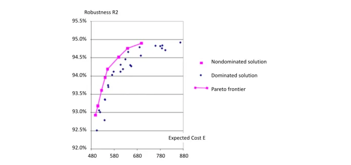
Using our Simulated Annealing algorithm, the project manager is able to change his objective function or decide to optimize a composite objective that is a weighted average of two or more objective functions (e.g., Expectation cost and Robustness function). By varying the weights, an approximation of the Pareto
Table 3: Computational results: large instances
Instances LP-based Heuristic SA1 SA2
N Nj Obj time(s) Obj time(s) Obj time(s)
3 10 153.46 4.13 144.08 186.01 101.08 1053.0 20 31.86 26.83 83.01 277.29 28.21 1631.0 50 299.18 884.94 187.55 722.52 4.63 3998.5 5 10 340.02 42.57 373.76 271.41 86.61 1531.6 20 90.69 67.95 63.41 412.01 22.16 2434.2 50 1.20 523.20 60.74 787.86 0.00 4562.1 7 10 227.01 51.50 214.85 337.20 48.28 1855.3 20 801.99 224.15 820.97 628.14 596.62 3289.0 50 79.61 467.90 139.58 1212.02 0.00 6869.1
frontier is obtained (Figure 5). A project manager can select one of the eight non-dominated solutions by making a trade-off between robustness and expected cost.
Nondominated solution Dominated solution Pareto frontier 95.5% 95.0% 94.5% 94.0% 93.5% 93.0% 92.5% 92.0% 480 580 680 780 880 Robustness R2 Expected Cost E
Figure 5: An approximation of the Pareto frontier: Nondominated solutions
Embedded in a decision support system (DSS), our FRCCP approach allows project managers to choose the solution that they assess to be the best amongst those forming the Pareto frontier. Before discussing how to interpret the model outcomes, we will explain the terminology that is common to using a fuzzy planning approach. In this context, the possibility framework is much more loose than the probabilistic one: • A possibility equal to one only means that the corresponding event is fully possible, but not at all that it is certain. We distinguish between ’possible’ and ’completely possible’, to indicate when the degree of possibility is non nul but less than one or equal to one.
• A necessity equal to one means that the corresponding event is certain or ’completely necessary’. When necessity is non nul but less than one, it means that the event is quite certain.
For each suitable solution on the Pareto frontier an associated fuzzy resource loading profile like in Figure 6 provides to managers a workload plan for all the concerned resources. This workload plan shows where additional (non-regular) capacity may be needed, given by the possibility and necessity that the workload is greater than the limits of capacity (regular, overtime and hired capacity). Using this workload plan, the managers can make arrangements and prepare decisions for ensuring a good workload / capacity balance, for example by warning subcontractors on the possibility of a later workload transfer, by evaluating the feasibility of increasing the capacity of the workshop, by workload smoothing, or by negotiating new delivery date with customer, etc [17]. We emphasize that some training has to be provided to managers to be able to properly interpret such information that comes from fuzzy modeling.
Periods
170 160
150 Fuzzy profile: Necessity
140 and possibility measures
130
120 Hiring capacity limit
110 Overtime capacity limit
100 regular capacity limit
90 80 P1 P2 P3 P4 P5 P6 P7 Periods Hours 170 160 150 140 130 120 110 100 90 80 70 60 A G B D C F E
Figure 6: A workload plan: a fuzzy resource loading profile for a resource type and a set of periods
Let us consider the example in Figure 6 and analyze the fuzzy workload in period 1. First, we remark that the uncertainty is important (workload between 82h5 and 165h i.e. interval ”A”). The capacity is not sufficient to absorb the workload. In fact, an overtime of 7h30 (i.e. interval ”B”) is ’completely necessary (i.e. certain), and additional 20h of overtime (i.e. interval ”C”) is ’necessary’ but not ’completely necessary’ (i.e. quite certain). An additional 5h of overtime (i.e. interval ”D”) and 35h of hiring extra operator (i.e. interval ”E”) are ’completely possible’. An additional 5h of hiring extra operator (i.e. interval ”F”) and 17H50 of outsourcing hours (i.e. interval ”G”) are ’possible’ but not ’completely possible’.
Of course, contrary to deterministic workload, information is not precise as we illustrated in Figure 6, and covers all situations with a quantification of their possibility of occurrence. This fuzzy workload allows making a decision on the base of an evaluation of the risk that the managers take while supposing that the real workload will have a given value. Imagine for example that the managers decide to request 37h50 of overtime and 5h of hiring extra operator so that the total workload becomes equal to 112h5, and finally this extra-workload is insufficient because the real workload to make the planned work at period 1 is 125h. In this case, the workload of 12h50 that is not carried out at period 1 should be carried out at period 2. The overtime hours, hiring extra operator (interim) hours and outsourcing hours are planned within a horizon of 1 week, 2 weeks and 4 weeks, respectively. Thus, for the workload that is not carried out in period 1, an equivalent workload will be carried out using regular capacity in period 2, overtime in periods 2 to 4, hiring in period 3 to 4 or outsourcing after period 4.
7. Conclusion
This paper explains how an RCCP problem under uncertainty can be modeled using the fuzzy/possibilistic approach. Some fuzzy objective functions are defined and a Simulated Annealing algorithm is provided to
solve the Fuzzy RCCP problem. The Simulated Annealing algorithm is compared to existing algorithms. These are a branch-and-price technique [19] and an LP-based heuristic [15]. For computational experimen-tation we have used benchmark instances from a shipyard maintenance center. Results of compuexperimen-tations are provided and show the performance of our metaheuristic. Finally, we have explained how the results of our algorithm can be exploited by project managers.
The future research will deal with the minimization of costs incurred by projects’ lateness in addition to the minimization of overcapacity cost. For this purpose, we plan to develop a fuzzy resource-driven approach and thus consider the fuzzy time-driven and the fuzzy resource driven approaches within a decisional loop handling projects due dates and production capacity simultaneously.
References
[1] Ibrahim Bakry. Optimized Scheduling of Repetitive Construction Projects under Uncertainty. PhD thesis, Concordia University, June 2014.
[2] Cynthia Barnhart, Ellis L. Johnson, George L. Nemhauser, Martin W. P. Savelsbergh, and Pamela H. Vance. Branch-and-price: Column generation for solving huge integer programs. Operations Research, 46(3):316–329, 1998.
[3] Tarun Bhaskar, Manabendra N. Pal, and Asim K. Pal. A heuristic method for RCPSP with fuzzy activity times. European Journal of Operational Research, 208(1):57–66, 2011.
[4] Shan-Huo Chen. Operations of fuzzy numbers with step form membership function using function principle. Information Sciences, 108(14):149 – 155, 1998.
[5] Shan Huo Chen, Shiu Tung Wang, and Shu Man Chang. Optimization of fuzzy production inventory model with repairable defective products under crisp or fuzzy production quantity. International Journal of Operations Research, 2(2):31–37, 2005.
[6] Shu-Jen Chen and Ching-Lai Hwang. Fuzzy Multiple Attribute Decision Making: Methods and Applications. Springer-Verlag New York, Inc., Secaucus, NJ, USA, 1992.
[7] Sophie Qinghong Chen. Comparing Probabilistic and Fuzzy Set Approaches for Designing in the Presence of Uncertainty. PhD thesis, Virginia Polytechnic Institute and State University, Blacksburg, Virginia, 2000.
[8] Ronald DeBoer. Resource-constrained Multi-Project Management - A Hierarchical Decision Support System. PhD thesis, BETA Institute for Business Engineering and Technology application, 1998.
[9] Didier Dubois and Henri Prade. The mean value of a fuzzy number. Fuzzy Sets and Systems, 24(3):279–300, December 1987.
[10] Didier Dubois and Henri Prade. Possibility Theory: An Approach to Computerized Processing of Uncertainty. Plenum Press, New York, 1988.
[11] Didier Dubois and Henri Prade. Fuzzy sets and probability: Misunderstandings, bridges and gaps. In Proceedings of the Second IEEE Conference on Fuzzy Systems, pages 1059–1068. IEEE, 1993.
[12] Salah E. Elmaghraby. Contribution to the round table discussion on new challenges in project scheduling. In PMS Conference, Valencia, Spain, April 3-5 2002.
[13] Juan Carlos Figueroa-Garca, Dusko Kalenatic, and Cesar Amilcar Lopez-Bello. Multi-period mixed production planning with uncertain demands: Fuzzy and interval fuzzy sets approach. Fuzzy Sets and Systems, 206(0):21 – 38, 2012. [14] Philippe Fortemps. Jobshop scheduling with imprecise durations: A fuzzy approach. IEEE Transactions on Fuzzy Systems,
5(4):557–569, November 1997.
[15] Noud Gademann and Marco Schutten. Linear-programming-based heuristics for project capacity planning. IIE Transac-tions, 37:153–165, 2005.
[16] Jun Gang, Jiuping Xu, and Yinfeng Xu. Multiproject resources allocation model under fuzzy random environment and its application to industrial equipment installation engineering. Journal of Applied Mathematics, page 19, 2013. [17] Laurent Geneste, Bernard Grabot, and Gabriel Reynoso-Castillo. Management of demand uncertainty within mrp ii using
possibility theory. In 16th IFAC World Congress, Czech Republic, 2005.
[18] Bernard Grabot, Laurent Geneste, Gabriel Reynoso Castillo, and Sophie V´erot. Integration of uncertain and imprecise orders in the MRP method. International Journal of Intelligent Manufacturing, 16(2):215–234, 2005.
[19] Erwin W. Hans. Resource Loading by Branch-and-Price Techniques. PhD thesis, Twente University Press, Enschede, Netherland, 2001.
[20] Erwin W. Hans, Willy Herroelen, Roel Leus, and Gerhard Wullink. A hierarchical approach to multi-project planning under uncertainty. Omega, 35:563–577, 2007.
[21] Willy Herroelen and Roel Leus. Project scheduling under uncertainty: Survey and research potentials. European Journal of Operational Research, 165(2):289–306, 2005.
[22] Scott Kirkpatrick, C. Daniel Gelatt, and Mario P. Vecchi. Optimization by simulated annealing. Science, 220:671–680, 1983.
[23] Tam´as Kis. A branch-and-cut algorithm for scheduling of projects with variable-intensity activities. Mathematical Pro-gramming, 103:515–539, July 2005.
[24] Bart Kosko. Fuzziness vs. probability. International Journal of General Systems, 17(2-3):211–240, 1990.
[25] Roel Leus. The generation of stable project plans, Complexity and Exact Algorithms. PhD thesis, Katholieke Universiteit Leuven, Leuven, Belgium, 2003.
[26] Xuesong Li, Hiroaki Ishii, and Minghao Chenr. Single machine parallel-batching scheduling problem with fuzzy due-date and fuzzy precedence relation. International Journal of Production Research, 53(9):2707–2717, 2015.
[27] Baoding Liu and Yian-Kui Liu. Expected value of fuzzy variable and fuzzy expected value models. IEEE Transactions on Fuzzy Systems, 10(4):445–450, august 2002.
[28] Malek Masmoudi and Alain Hait. Fuzzy uncertainty modelling for project planning: application to helicopter maintenance. International Journal of Production Research, 50(13):3594–3611, 2012.
[29] Malek Masmoudi and Alain Hait. Project scheduling under uncertainty using fuzzy modelling and solving techniques. Engineering Applications of Artificial Intelligence, 26(1):135–149, 2013.
[30] Malek Masmoudi, Erwin W. Hans, and Alain Hait. Fuzzy tactical project planning: Application to helicopter maintenance. In the 16th IEEE International Conference on Emerging Technologies and Factory Automation ETFA’2011, Toulouse, France, September 2011.
[31] Gilles Mauris. A comparison of possibility and probability approaches for modelling poor knowledge on measurement distribution. In Instrumentation and Measurement Technology Conference Proceedings, 2007. IMTC 2007. IEEE, pages 1–5, may 2007.
[32] Mohammad Saidi Mehrabad and Ali Pahlavani. A fuzzy multi-objective programming for scheduling of weighted jobs on a single machine. The International Journal of Advanced Manufacturing Technology, 45:122139, 2009.
[33] Ozcan Mutlu and Elif Ozgormus. A fuzzy assembly line balancing problem with physical workload constraints. Interna-tional Journal of Production Research, 50(18):5281–5291, 2012.
[34] Muhammad Nazim, Muhammad Hashim, and Jiuping Xu. Multi objective optimization of production-distribution problem under fuzzy random environment. Global Journal of Technology & Optimization, 5(1), 2014.
[35] Efstratios Nikolaidis, Sophie Chen, Harley Cudney, Raphael T. Haftka, and Raluca Rosca. Comparison of probability and possibility for design against catastrophic failure under uncertainty. Journal of Mechanical Design, 126(3):386–394, 2004. [36] Fabrice Talla Nobibon, Roel Leus, Kameng Nip, and Zhenbo Wang. Resource loading: Applications and complexity analysis. In 11th International Symposium on Operations Research and its Applications in Engineering, Technology and Management 2013 (ISORA 2013), pages 1–5, August 2013.
[37] David Peidro, Josefa Mula, Mariano Jimnez, and Ma del Mar Botella. A fuzzy linear programming based approach for tactical supply chain planning in an uncertainty environment. European Journal of Operational Research, 205(1):65 – 80, 2010.
[38] Masatoshi Sakawa and Ryo Kubota. Fuzzy programming for multiobjective job shop scheduling with fuzzy processing time and fuzzy duedate through genetic algorithms. European Journal of Operational Research, 120(2):393–407, 2000. [39] Xueyan Song and Sanja Petrovic. A fuzzy approach to capacitated flow shop scheduling. In the 11th International
Conference on Information Processing and Management of Uncertainty in Knowledge-based Systems, IPMU, pages 486– 493, Paris, July 2006.
[40] Y. Sotskov and F. (Eds.) Werner. Sequencing and scheduling with inaccurate data. New York Nova Publishers, Hauppauge, New York, 2014.
[41] Paul Tannery and Charles Henry. Oeuvres de Fermat, volume 2. Gauthier Villars, Paris, 1894.
[42] Seyed .A. Torabi, Mahmoud Ebadian, and Reza Tanha. Fuzzy hierarchical production planning (with a case study). Fuzzy Sets and Systems, 161(11):1511 – 1529, 2010.
[43] Peter J. M. van Laarhoven, Emile H. L. Aarts, and Jan Karel Lenstra. Job shop scheduling by simulated annealing. Operations Research, 40(1):113–125, 1992.
[44] Reay-Chen Wang and Hsiao-Hua Fang. Aggregate production planning with multiple objectives in a fuzzy environment. European Journal of Operational Research, 133(3):521 – 536, 2001.
[45] Bo K. Wong and Vincent S. Lai. A survey of the application of fuzzy set theory in production and operations management: 1998-2009. International Journal of Production Economics, 129(1):157–168, January 2011.
[46] Gerhard Wullink. Resource Loading Under Uncertainty. PhD thesis, Twente University Press, Enschede, Netherland, 2005.
[47] Gerhard Wullink, Noud Gademann, Erwin W. Hans, and Aart van Harten. A scenario based approach for flexible resource loading under uncertainty. International Journal of Production Research, 42(24):5079–5098, 2004.
[48] Lotfi Askar Zadeh. Fuzzy sets. Information and Control, 8:338–353, 1965.
[49] Lotfi Askar Zadeh. Fuzzy sets as basis for a theory of possibility. Fuzzy Sets and Systems, 1:3–28, 1978.
[50] Lotfi Askar Zadeh. Discussion: Probability theory and fuzzy logic are complementary rather than competitive. Techno-metrics, 37(3):271–276, 1995.
View publication stats View publication stats