HAL Id: tel-01895859
https://tel.archives-ouvertes.fr/tel-01895859
Submitted on 15 Oct 2018
HAL is a multi-disciplinary open access archive for the deposit and dissemination of sci-entific research documents, whether they are pub-lished or not. The documents may come from teaching and research institutions in France or abroad, or from public or private research centers.
L’archive ouverte pluridisciplinaire HAL, est destinée au dépôt et à la diffusion de documents scientifiques de niveau recherche, publiés ou non, émanant des établissements d’enseignement et de recherche français ou étrangers, des laboratoires publics ou privés.
lambda-calculus
Pierre Vial
To cite this version:
Pierre Vial. Non-idempotent typing operators, beyond the lambda-calculus. Computation and Lan-guage [cs.CL]. Université Sorbonne Paris Cité, 2017. English. �NNT : 2017USPCC038�. �tel-01895859�
Thèse de doctorat de l’Université Sorbonne Paris Cité Préparée à l’Université Paris Diderot
Ecole Doctorale 386 — Sciences Mathématiques de Paris Centre Institut de recherche en informatique fondamentale (I.R.I.F.)
équipe Preuves Programmes Systèmes
Opérateurs de typage
non-idempotents, au-delà du
λ-calcul
par Pierre Vial
Thèse de doctorat d’informatique dirigée par
Delia Kesner Directrice de thèse
Damiano Mazza Co-directeur de thèse
Thèse soutenue publiquement le 7 décembre 2017 devant le jury constitué de
Directrice de thèse Kesner Delia Professeur Paris Diderot Rapporteur Klop Jan Willem Professeur émérite Vrije Universiteit Examinateur dal Lago Ugo Maître de conférence Università di Bologna Chargé de Recherche Mazza Damiano Co-directeur de thèse Paris 13
Examinatrice van Raamsdonk Femke Maître de conférence Vrije Universiteit Président du Jury Regnier Laurent Professeur Université Aix-Marseille Rapporteur Rehof Jakob Professeur TU Dortmund
Pierre Vial Thèse de Doctorat 20171
Opérateurs de typage non-idempotents, au delà du λ-calcul
Contributions: L’objet de cette thèse est l’extension des méthodes de la théorie des types intersections non-idempotents, introduite par Gardner et de Carvalho, à des cadres dépassant le λ-calcul stricto sensu.
• Nous proposons d’abord une caractérisation de la normalisation de tête et de la normalisation forte du λµ-calcul (déduction naturelle classique) en introduisant des types unions non-idempotents. Comme dans le cas intuitionniste, la non-idempotence nous permet d’extraire du typage des informations quantitatives ainsi que des preuves de terminaison beaucoup plus élémentaires que dans le cas idem-potent. Ces résultats nous conduisent à définir une variante à petits pas du λµ– calcul, dans lequel la normalisation forte est aussi caractérisée avec des méthodes quantitatives.
• Dans un deuxième temps, nous étendons la caractérisation de la normalisation faible dans le λ-calcul pur à un λ-calcul infinitaire étroitement lié aux arbres de Böhm et dû à Klop et al. Ceci donne une réponse positive à une question connue comme le problème de Klop. À cette fin, il est nécessaire d’introduire conjointe-ment un système (système S) de types infinis utilisant une intersection que nous qualifions de séquentielle, et un critère de validité servant à se débarrasser des preuves dégénérées auxquelles les grammaires coinductives de types donnent nais-sance. Ceci nous permet aussi de donner une solution au problème 20 de TLCA (caractérisation par les types des permutations héréditaires). Il est à noter que ces deux problèmes n’ont pas de solution dans le cas fini (Tatsuta, 2007).
• Enfin, nous étudions le pouvoir expressif des grammaires coinductives de types, en dehors de tout critère de validité. Nous devons encore recourir au système S et nous montrons que tout terme est typable de façon non triviale avec des types in-finis et que l’on peut extraire de ces typages des informations sémantiques comme l’ordre (arité) de n’importe quel λ-terme. Ceci nous amène à introduire une méth-ode permettant de typer des termes totalement non-productifs, dits termes muets, inspirée de la logique du premier ordre. Ce résultat prouve que, dans l’extension coinductive du modèle relationnel, tout terme a une interprétation non vide. En utilisant une méthode similaire, nous montrons aussi que le système S collapse surjectivement sur l’ensemble des points de ce modèle.
Mots-clés: lambda calcul, type, non-idempotent, type intersection, typage infinitaire, coinduction, intersection séquentielle, type rigide, lambda-mu calcul, logique classique, Curry-Howard, collapse, réduction productive, réduction non-productive
Non-idempotent typing operators, beyon the λ-calculus
Abstract In this dissertation, we extend the methods of non-idempotent intersection type theory, pioneered by Gardner and de Carvalho, to some calculi beyond the λ-calculus.
• We first present a characterization of head and strong normalization in the λµ calculus (classical natural deduction) by introducing non-idempotent union types. As in the intuitionistic case, non-idempotency allows us to extract quantitative information from the typing derivations and we obtain proofs of termination that are far more elementary than those in the idempotent case. These results leads us to define a small-step variant of the λµ calculus, in which strong normalization is also characterized by means of quantitative methods.
• In the second part of the dissertation, we extend the characterization of weak nor-malization in the pure λ-calculus to an infinitary λ-calculus narrowly related to Böhm trees, which was introduced by Klop et al. This gives a positive answer to a question known as Klop’s problem. In that purpose, it is necessary to simulta-neously introduce a system (system S) featuring infinite types and resorting to an intersection operator that we call sequential, and a validity criterion in order to discard unsound proofs that coinductive grammars give rise to. This also allows us to give a solution to TLCA problem # 20 (type-theoretic characterization of hereditary permutations). It is to be noted that those two problem do not have a solution in the finite case (Tatsuta, 2007).
• Finally, we study the expressive power of coinductive type grammars, without any validity criterion. We must once more resort to system S and we show that every term is typable in a non-trivial way with infinite types and that one can extract semantical information from those typings e.g. the order (arity) of any λ-term. This leads us to introduce a method that allows typing totally unproductive terms (the so-called mute terms), which is inspired from first order logic. This result es-tablishes that, in the coinductive extension of the relational model, every term has a non-empty interpretation. Using a similar method, we also prove that system S surjectively collapses on the set of points of this model.
Key words: lambda calculus, type, non-idempotent, intersection type, infinitary typ-ing, coinduction, sequential intersection, rigid type, lambda-mu calculus, classical-logic, Curry-Howard, collapse, productive reduction, non-productive reduction
Pierre Vial Thèse de Doctorat 20173
Marcelle Nullans 10 février 1931 - 21 août 2017
In Memoriam
Cette thèse est dédiée à ma grand-mère, Marcelle Nullans,
en mémoire de sa générosité, de sa bienveillance et de tout ce qu’elle m’a appris.
Remerciements
Mes remerciements vont d’abord à Delia Kesner, qui a accepté de me diriger en thèse environ un quart d’heure après m’avoir rencontré et a bien voulu composer un sujet à quatre mains en un temps record avant l’heure limite de remise des projets! Je suis aussi redevable à Delia de m’avoir posé la question qui devait être reconnue a posteriori comme le problème de Klop: c’est de là que presque tout est parti. Pendant ces trois années de thèse, Delia m’a prodigué ses conseils et a fait preuve d’une infinie patience pour lire et relire encore un grand nombre de versions de mes articles et de mon manuscrit, dont certaines étaient peut-être, avouons-le, un peu thomas-bernhardiennes.
Merci à Damiano Mazza de m’avoir d’abord encadré en stage “d’initiation à la recherche” en M2 et pour son enthousiasme communicatif, ses mille idées qui surgis-sent à chaque instant. Merci aussi pour la confiance et la liberté offerte pendant ces trois ans et demi, ses nombreux encouragements et pour m’avoir en premier orienté vers le λ-calcul infini !
Jan Willem Klop et Jakob Rehof m’ont fait l’honneur de bien vouloir être les rappor-teurs de ma thèse. Je les remercie pour tout le temps et tous les efforts consacrés à lire l’intégralité du manuscrit, et pour les remarques détaillées qu’ils ont bien voulu me faire sur celui-ci. Je n’ose pas penser que cela a été une sinécure. Merci à Jan Willem Klop, pour avoir, avec d’autres, inventé le λ-calcul infinitaire et à Jakob Rehof pour les très agréables moments de discussion que nous avons eus à Budapest, Reykjavik ou Oxford. Que Ugo dal Lago, Femke van Raamsdonk et Laurent Regnier soient aussi remerciés d’avoir bien voulu faire partie de mon jury de thèse.
Je remercie Alexis Saurin, aussi bien l’ami, le responsable des thésards aux conseils avisés que le chercheur avec qui j’ai eu de nombreuses discussions éclairantes, notam-ment à travers sa connaissance et sa compréhension encyclopédiques des langages de programmation, qui vont bien au delà du λ-calcul.
Ma gratitude va aussi à Giulio Manzonetto, qui a parfois pris la casquette de co-co-directeur de thèse et s’est intéressé à ce qui constitue la dernière partie de ma thèse. Giulio a notamment relu plusieurs articles qui constituent la fin de ce manuscrit et j’ai profité extensivement de ses conseils en rédaction (et en typographie) scientifique. Je re-mercie aussi tous les chercheurs1avec qui j’ai eu des discussions scientifiques éclairantes: je pense notamment à Daniel de Carvalho, Antonio Bucciarelli, Thomas Ehrhard, Hugo Herbelin, Paul-André Melliès, Roman Péchoux, Matthieu Sozeau, Christine Tasson et Lionel Vaux.
Merci à Odile Ainardi et à Marie Fontanillas pour leur patience quasi-bouddhique et pour toute l’efficacité qu’elles ont déployée pendant mes missions et déplacements en
1
Selon la tradition, les précaires seront remerciés dans un deuxième temps. 5
France et à l’étranger, pour moi, comme pour tout le monde.
Le LMFI a été riche en rencontres. Je remercie Amina2 Doumane, dont l’amitié a été très précieuse depuis que nous nous connaissons. Merci pareillement à Ludovic Patey, l’homme qui a le CNRS plusieurs fois chaque année, avec qui je ne compte plus les discussions de toutes sortes, autour d’un feu de camp ou ou d’un bassin rempli de poissons rouges. Je remercie Sonia Marin pour toutes ces heures passées sur les devoirs à la maison du LMFI et sur la géométrie filipendulaire (qui n’a rien à envier à la géométrie grothendieckienne).
Je remercie Charles Grellois de m’avoir fait profiter de sa culture scientifique, de ses slides et de ses conseils avisés, pour traverser les différentes ordalies que le thésard doit connaître avant de pouvoir soutenir. Merci à Cyrille Chenavier pour ses explications his-toriques sur la rivalité entre Attila et Charles Quint ou Hugues Capet, et pour ne toujours faire ressortir que la meilleure partie de chacun (et le faire savoir). Je ne dirai pas de mal d’Étienne Miquey, dernier compagnon3 de ligne gauche, car nous sommes appelés à nous revoir assez régulièrement dans un futur proche. Il faut quand même reconnaître que ses explications sur la logique classique et les types dépendants n’étaient pas inintéres-santes. Merci à Maxime Lucas pour sa loquacité, et à Antoine Allioux pour sa résistance à l’alcool. Merci à Léonard Guetta pour sa magnanimité et son couscous à venir4. Merci à tous les autres thésards et stagiaires de l’IRIF, d’aujourd’hui ou d’hier: Clément Jacq (qui était de facto co-directeur de PPS), Thibaut Girka, Pierre-Marie Pedrot, Yann Ham-daoui, Gabriel Radanne, Théo Zimmermann, Tommaso Petrucciani,Théo Winterhalter, Nicolas Jeannerod, Victor Lanvin, Leo Stefanesco, Zeinab Galal, Jules Chouquet, Chai-tanya Leena Subramaniam, Rémi Nollet, Cédric Ho Tanh, Matthieu Bouttier, Hadrien Batmalle, Raphaëlle Crubillé, Cyprien Mangin, Thibault Godin, Pierre Cagne et Adrien Husson. Merci aux doctorantes honoris causa, Clémentine, Daniel et Maud. Je n’oublie pas les thésards de Paris 13, Luc Pellissier, Alice Pavaux et Thomas Rubiano, avec qui je suis allé notamment à OPLSS, et plus encore, à Hot Cougar Springs. Toute ma grat-itude politico-culturelle à Luc, qui m’a fait connaître Thomas Römer, les Brigandes et Liza Monet.
J’ai rencontré des professeurs exceptionnels à l’École normale supérieure, comme François Loeser, Jean-François Le Gall, Marc Rosso, quoique mon assiduité ne m’ait pas fait profiter de leurs enseignements autant qu’ils le méritaient. Marc Rosso a accepté de me recevoir au printemps 2012 alors que je m’interrogeais sur une réinscription à l’Université et m’a orienté vers le LMFI. Arnaud Durand a ensuite bien voulu accepter ma candidature et j’ai pu commencer les cours le lendemain de notre entretien le mois de septembre suivant. À tous les deux, merci.
Au cours de ma scolarité, j’ai eu la chance d’être élève dans la classe de Mme Alini, en CP et CE1 à l’école des Cités-Cécile, ainsi que celle de Mlle Welter et M. Dupuy, au collège Charles Guérin de Lunéville. Je leur exprime ma gratitude, pour m’avoir montré ce qu’était un cours vivant et à l’écoute5 des élèves. Merci aussi à Philippe Château, mon professeur en MP* au lycée Henri Poincaré. De l’autre côté du miroir, il me faut
2
Qu’elle n’oublie pas cependant les pièces de tissu simples et de bon goût qu’elle a promises à une bonne partie des membres de l’IRIF du bas.
3
Quoiqu’il ait, contrairement à l’auteur, astucieusement évité les frais de réinscription en “4ème année”.
4
Le couscous est à venir, pas la magnanimité, qui n’est plus à prouver
5Pour l’improbable lecteur qui aurait eu la chance de fréquenter l’IUFM et autres ESPE, cette
Pierre Vial Thèse de Doctorat 20177
remercier mes anciens élèves, sur qui j’ai expérimenté toutes les méthodes de travail qui me faisaient défaut. Sans eux, je n’aurais sans doute pas pu mettre le pied à l’étrier.
Enfin, un grand merci à Nicolas Tabareau de m’accueillir à Nantes pour une année de post-doc. C’est une immense opportunité de découvrir Coq et la théorie homotopique des types avec lui.
Reprendre les études n’a pas été de soi. Sans les nombreux encouragements de Camille Tauveron, Jean-Baptiste Bilger, Julien Rabachou, Hélène Valance, Sandra Collet et Stéphane Pouyaud, je n’aurais sans doute jamais dépassé mes hésitations et retrouvé le chemin des écoliers. Qu’ils soient tous remerciés pour m’avoir accompagné un moment ou un autre. Pour la même raison, je remercie aussi Michel Plouznikoff. Merci à Shirine, Marie-Cécile, David et Rossella pour leur amitié.
Mes années de thèse auraient été traversées bien différemment si Mahek ne m’avait pas apporté l’Illumination quelques heures avant un départ en avion: je lui en serai toujours reconnaissant. Je suis particulièrement redevable à la famille Rollet, à Fanny et à Christine en particulier, de m’avoir chaleureusement accueilli au printemps 2015. Je remercie aussi Joseph Beaume pour son amitié, ainsi que pour les nombreux livres qu’il m’a envoyés. Ma reconnaissance aussi à Rachel Daniel, pour sa compréhension profonde des expériences intérieures. Merci à Mariana pour les dernières semaines de septembre, alors que j’apportais les touches finales à ce manuscrit. Merci à Mathilde Régent et Aude Leblond, pour leur voisinesque et verre-siffleuse présence pendant ces trois années, matérialisée par d’innombrables tisanes, bières, vodkas et autres Yogi Teas c.
Je remercie mes soeurs, Mélanie et Camille, pour tout ce que j’ai partagé avec elles, à Paris, à Lunéville ou en Bretagne. Enfin, je remercie mes parents pour le soutien qu’ils m’ont apporté tout au long de ma reprise d’études.
Contents
Contents 9
1 Introduction 15
1.1 Functions and Termination . . . 17
1.2 Processing Computation in Functional Programming . . . 21
1.3 Intersection (or not) Types in the λ-Calculus . . . 26
1.4 Infinitary Computation, Coinduction and Productivity . . . 34
1.5 Main Contributions (Technical Summary) . . . 38
1.6 How to read this thesis . . . 41
I PRELIMINARIES 43 2 Lambda Calculus 47 2.1 Pure Lambda Calculus . . . 48
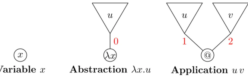
2.1.1 Tracks and Labelled Trees . . . 48
2.1.2 Lambda Terms and Alpha Equivalence . . . 51
2.1.3 Beta Reduction, Redexes and Normal Forms . . . 53
2.1.4 Notable Lambda Terms . . . 54
2.1.5 Residuals and Quasi-Residuals . . . 55
2.1.6 Reduction Sequences and Residuation . . . 58
2.1.7 Contexts . . . 58
2.2 Normalizations and Reduction Strategies . . . 59
2.2.1 Head Redexes, Head Normal Forms, Head Reduction . . . 60
2.2.2 Weak Normalization and Leftmost Reduction . . . 61
2.2.3 Strong Normalization . . . 63
2.3 Tinkering with Normalization . . . 63
2.3.1 Stable Positions and Sets of Normal Forms . . . 64
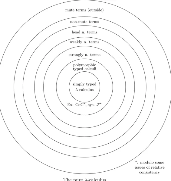
2.3.2 Mute Terms and Order of a Lambda Term . . . 65
2.3.3 Toward Infinitary Normalization . . . 66
2.3.4 Partial Normal Forms . . . 68
2.3.5 Böhm Reduction Strategies . . . 70
2.4 A Lambda-Calculus with Explicit Substitutions . . . 72
3 Intersection Type Systems 75 3.1 From the λ-Calculus to Intersection Types Theory . . . 76
3.1.1 The Curry-Howard Correspondence . . . 76
3.1.2 Lambda-Calculus and Type Theory . . . 76
3.1.3 A Simple Type System . . . 78
3.1.4 Types and Termination . . . 79
3.2 Principles and Examples of Intersection Types . . . 80
3.2.1 Towards Strictness and Relevance . . . 80
3.2.2 Intersection Operator, Sets and Multisets . . . 83
3.2.3 SystemD0 (Idempotent Intersection) . . . 85
3.2.4 SystemR0 (Non-Idempotent Intersection) . . . 86
3.3 Discussing Subject Reduction and Subject Expansion . . . 87
3.3.1 Uses and Behaviors of Intersection Type Systems . . . 88
3.3.2 Subject Reduction and Subject Expansion . . . 89
3.3.3 Context Preservation . . . 91
3.3.4 Failure of Subject Expansion with Relevant Idempotent Intersection 93 3.3.5 Weakening and Irrelevant Intersection Types Systems . . . 94
3.4 Study of Head Normalization in System R0 . . . 97
3.4.1 Typed and Untyped Parts of a Term . . . 97
3.4.2 Typing (Head) Normal Forms . . . 98
3.4.3 Weighted Subject Reduction . . . 101
3.4.4 Characterization of Head Normalization and Completeness of Head Reduction . . . 101
3.4.5 Order Discrimination . . . 102
4 A Few Complements on Intersection Types 105 4.1 A Bit of This and a Bit of That . . . 105
4.1.1 An Alternative Presentation of Relevant Derivations . . . 105
4.1.2 Confluence (and Non-Confluence) of Type Systems . . . 106
4.1.3 Type Systems and their Features (Summary) . . . 109
4.2 Intersection Types for the Lambda Calculus with Explicit Substitutions 109 4.3 Tait’s Realizability Argument . . . 111
4.3.1 The Failure of an Induction . . . 111
4.3.2 Interpretation . . . 113
5 Characterizing Weak and Strong Normalization 117 5.1 Characterizing Weak Normalization . . . 117
5.1.1 Positive and Negative Occurrence of a Type . . . 117
5.1.2 Unforgetfulness . . . 118
5.1.3 Unforgetfulness and Typing Rules . . . 119
5.1.4 Weak Normalization . . . 121
5.2 Characterizing Strong Normalization . . . 122
5.2.1 Erasable Subterms . . . 122
5.2.2 Subject Reduction and Expansion in S . . . 124
5.2.3 Strong Normalization as an Inductive Predicate . . . 125
5.2.4 Characterizing Strong Normalization . . . 127
5.2.5 Obtaining an Upper Bound for Normalizing Sequence . . . 128
II RESOURCES FOR CLASSICAL NATURAL DEDUCTION 131 Presentation . . . 133
CONTENTS 11
6 The Lambda-Mu Calculus 135
6.1 Classical Logic in Natural Deduction . . . 135
6.1.1 Getting Classical Logic . . . 135
6.1.2 Focused Classical Natural Deduction . . . 136
6.2 The Lamda-Mu Calculus . . . 137
6.2.1 Lambda-Mu Terms . . . 138
6.2.2 Simply Typed Lambda-Mu Calculus . . . 139
6.2.3 Operational Semantics . . . 139
6.2.4 Subject Reduction for Simply Typed Lambda-Mu . . . 140
6.2.5 Normalization in Lambda-Mu Calculus . . . 141
7 Non-Idempotent Intersection and Union Types for Lambda-Mu 143 7.1 Auxiliary Judgments and Choice Operators . . . 144
7.2 Quantitative Type Systems for the λµ-Calculus . . . 147
7.2.1 Types . . . 147 7.2.2 System Hλµ . . . 148 7.2.3 Design of System Hλµ . . . 151 7.2.4 System Sλµ . . . 153 7.3 Typing Properties . . . 154 7.3.1 Forward Properties . . . 154 7.3.2 Backward Properties . . . 160
7.4 Strongly Normalizing λµ-Objects . . . 164
7.5 Relevance (an Inquiry) . . . 167
8 A Resource Aware Semantics for the Lambda-Mu-Calculus 169 8.1 The λµr-calculus . . . 169 8.1.1 Syntax . . . 170 8.1.2 Operational Semantics . . . 171 8.1.3 Typing System . . . 171 8.2 Typing Properties . . . 173 8.2.1 Forward Properties . . . 173 8.2.2 Backward Properties . . . 178
8.3 Strongly Normalizing λµr-Objects . . . 182
8.4 Conclusion . . . 184
IIIINFINITARY NORMALIZATION AND SEQUENTIAL INTER-SECTION 185 Presentation . . . 187
9 The Infinitary Lambda-Calculus 189 9.1 Böhm Trees . . . 189
9.2 Induction and Coinduction . . . 191
9.2.1 Infinite Labelled Trees . . . 191
9.2.2 Smallest and Biggest Invariant Subsets . . . 192
9.2.3 Inductive vs. Coinductive Grammars . . . 192
9.3 The Infinitary Lambda Calculi . . . 194
9.3.1 The Full Infinitary Calculus . . . 194
9.3.2 The Infinitary Calculus of Böhm Trees . . . 198
10 Klop’s Problem 203
10.1 How to Answer Positively to Klop’s Problem . . . 206
10.1.1 The Finitary Type SystemR0 and Unforgetfulness . . . 206
10.1.2 Finitarily Typing the Infinite Terms . . . 207
10.1.3 Infinitary Subject Expansion by Means of Truncation . . . 209
10.2 Intersection by means of Sequences . . . 211
10.2.1 Towards System S . . . 212
10.2.2 Rigid Types . . . 213
10.2.3 Rigid Derivations . . . 214
10.3 Statics and Dynamics . . . 216
10.3.1 Bipositions and Bisupport . . . 216
10.3.2 Quantitativity and Coinduction . . . 217
10.3.3 One Step Subject Reduction and Expansion . . . 217
10.3.4 Safe Truncations of Typing Derivations . . . 220
10.3.5 A Proof of the Subject Reduction Property . . . 221
10.4 Approximable Derivations and Unforgetfulness . . . 222
10.4.1 The Lattice of Approximation . . . 222
10.4.2 Approximability . . . 223
10.4.3 Unforgetfulness . . . 224
10.4.4 The infinitary Subject Reduction Property . . . 226
10.5 Typing Normal Forms and Subject Expansion . . . 227
10.5.1 Support Candidates . . . 228
10.5.2 Natural Extensions . . . 229
10.5.3 Approximability . . . 230
10.5.4 The Infinitary Subject Expansion Property . . . 231
10.6 Conclusion . . . 232
IV UNDERSTANDING UNPRODUCTIVE REDUCTION THROUGH LOGICAL METHODS 233 Presentation . . . 235
11 An Informal Presentation of Threads 239 11.1 Threads, Syntactic Polarity and Consumption . . . 239
11.1.1 Ascendance, Polar Inversion and Threads . . . 239
11.1.2 Syntactic Polarity and Consumption . . . 241
11.1.3 Referents of Threads, Applicative Depth and Brotherhood . . . . 244
11.2 Collapsing Redex Towers . . . 246
11.2.1 Negative Left-Consumption and Redex Towers . . . 246
11.2.2 Collapsing a Redex Tower Sequence . . . 248
11.3 Formalizing Ascendance and Polar Inversion in System S . . . 250
11.3.1 Applications and Tracking in System S . . . 250
11.3.2 Abstractions and Tracking in System S . . . 251
12 Complete Unsoundness: a Linearization of the λ-Calculus 253 12.1 Coinductive Type Systems . . . 256
12.1.1 A Coinductive Simple Type System . . . 256
12.1.2 Complete Unsoundness and Relevance . . . 256
CONTENTS 13
12.1.4 Type System S (Sequential Intersection) . . . 258
12.2 Bisupport Candidates . . . 260
12.2.1 A Toy Example: Support Candidates for Types . . . 260
12.2.2 Toward the Characterization of Bisupport Candidates . . . 261
12.2.3 Tracking a Type in a Derivation . . . 262
12.2.4 Type Formation, Type Destruction . . . 265
12.2.5 Threads and Minimal Bisupport Candidate . . . 266
12.3 Nihilating Chains . . . 269
12.3.1 Polarity and Threads . . . 269
12.3.2 Interactions in Normal Chains . . . 271
12.3.3 Complete Unsoundness (almost) at Hand . . . 274
12.4 Normalizing Nihilating Chains . . . 275
12.4.1 Quasi-Residuals . . . 276
12.4.2 The Collapsing Strategy . . . 280
12.4.3 Redex Towers . . . 280
12.5 Applications . . . 282
13 The Surjectivity of the Collapse of Sequential Intersection Types 287 13.1 From Representing Types in System S to Representing Derivations . . . 290
13.1.1 Multiset Types as Collapses of Sequential Types . . . 290
13.1.2 The Representation Theorem and Hybrid Derivations . . . 293
13.1.3 SystemR and the Hybrid Construction . . . 295
13.2 Subject Reduction . . . 296
13.2.1 Encoding Reduction Choices with Interfaces . . . 296
13.2.2 Residuation and Encoding Reduction Choices . . . 298
13.3 Representation Theorem and Isomorphisms of Derivations . . . 299
13.3.1 Isomorphisms of Operable Derivations . . . 300
13.3.2 Resetting an Operable Derivation . . . 301
13.3.3 Relabelling a derivation . . . 302
13.4 Edge Threads . . . 304
13.4.1 Threads and Consumption of Mutable Edges . . . 305
13.4.2 Edge Threads and Syntactic Polarity . . . 307
13.4.3 Brother Chains and Representation . . . 307
13.4.4 Towards the Final Stages of the Proof . . . 309
13.4.5 Top Ascendants, Syntactic Polarity and Referents . . . 310
13.5 Residuation of Threads and the Collapsing Strategy . . . 313
13.5.1 Edges and Residuation . . . 314
13.5.2 The Collapsing Strategy for Operable Derivations . . . 315
13.5.3 Conclusion of the Proof . . . 315
13.6 Conclusion . . . 317
Conclusion 319 Bibliography 323 A Complements to Klop’s Problem 333 A.1 Expanding the Π0nand Π0 . . . 333
A.2 Equinecessity, Reduction and Approximability . . . 336
A.2.1 Equinecessary bipositions . . . 336
A.2.3 Equinecessity and Bipositions of Null Applicative Depth . . . 337
A.3 Lattices of (finite or not) approximations . . . 338
A.3.1 Meets and Joins of Derivations Families . . . 342
A.3.2 Reach of a derivation . . . 343
A.3.3 Proof of the subject expansion property . . . 344
A.4 Approximability of the quantitative NF-derivations . . . 344
A.4.1 Degree of a position inside a type in a derivation . . . 344
A.4.2 Truncation of degree n . . . 345
A.4.3 A Complete Sequence of Derivation Approximations . . . 347
A.5 Isomorphisms between S-Derivations . . . 347
A.6 Approximability cannot be defined by means of Multisets . . . 349
A.6.1 Quantitativity in SystemR . . . 349
A.6.2 Representatives and Dynamics . . . 349
A.7 A Positive Answer to TLCA Problem 20 . . . 351
B Residuation, Threads and Isomorphisms in System Sop 355 B.1 Subject Reduction . . . 355
B.1.1 Residual Derivation (Hybrid) . . . 356
B.1.2 Residual Types and Contexts (Hybrid Derivations) . . . 357
B.1.3 Residual Interface . . . 359
B.1.4 Proof of the Representation Lemma . . . 361
B.2 Isomorphisms and Relabelling of Derivations . . . 362
B.2.1 Isomorphisms of Operable Derivations . . . 362
B.2.2 Resetting an Operable Derivation . . . 363
B.3 Edge Threads, Brotherhood and Consumption . . . 364
B.4 Residuation for Mutable Edges and Threads . . . 365
B.4.1 Edges and Residuation . . . 365
Chapter 1
Introduction
Mise en bouche
This thesis is about the relations between type theory and mathematical logic. We specialize into the non-idempotent intersection type theory applied to the λ-calculus. Type theory provides syntactic certificates that some programs behave well e.g., terminate and the λ-calculus can be seen as the mold on which functional pro-gramming is designed. Thus, forgetting temporarily about the words “intersection” and “non-idempotent”, we are interested in finding guarantees that some programs of a lan-guage called the λ-calculus terminate.
The matter of finding such certificates of good behavior is indeed fundamental when working with expressive programming languages and it is a crucial step for having pro-grams that meet their specification: the specification of a program is everything what it is supposed to do e.g., you do not want the embedded system of your aircraft to open the doors while it is flying1 or to bug because of an unnoticed coding mistake)
The syntactic nature of the certificates – meaning that they rely on the source code– provided by type theory is an invaluable asset: this avoids all coding mistakes, contrary to semi-random benchmarking methods that only sample the instances of a program. As it turns out, type theory also ensures that streams – i.e. programs running without limit of time – keep on producing computations instead e.g., of looping in a cycle of states.
But what is a type? Roughly speaking, typing is a very simple idea: it just consists in describing what kind of data (integer? floating number? string of characters? array of integers? function?) is stored in the memory (in the variables) used by the program. We may then assign types to programs e.g., the function sumLength that takes two strings s1 and s2and outputs the sum of their respective lengths has the type (String×String) → int. On the left-hand side (the source), we find the types of the inputs2 and on its right-hand side (the target ), the type of the output. From the practical perspective, typing provides a form of safety for the program developer: one cannot inadvertently switch the name of an integer variable with that of a string variable without having an error, whereas some untyped languages may let the mistake pass unbeknownst to the programmer.
It is not this kind of type-safety we are interested in in this thesis, but that of the types as a guarantee of termination. But how does such a guarantee hold? Here is where
1Except if you are Tom Cruise. 2
Separated by the operator ×, roughly corresponding to a cartesian product. 15
mathematical logic comes into play. William A. Howard, extending some observations by Haskell Curry, noticed that type systems really look like some inference systems coming from mathematics, not only because assignment rules of types system and inference rules of logic are oddly similar (statical correspondence), but also because the execution-steps of programs are in almost every point homologous to the so-called cut-elimination steps (dynamical correspondence). As we will see, the cut-elimination procedure was introduced by Gerhard Gentzen [45] to give a (partial) proof of coherence of some logic underlying arithmetic: from a high-level perspective, this procedure consists in transforming a proof of an assertion A subdivided in several lemmas into a self-contained one-block proof of the same statement A.
An interesting aspect of Gentzen’s contribution, later extended to intuitionistic3 Nat-ural Deduction by Prawitz [95], is that he proved that this cut-elimination procedure is terminating. As a consequence of the correspondence developed by Curry and Howard (the so called Curry-Howard correspondence), the fact that the typed programs (w.r.t. some type systems) are terminating became a straightforward consequence of some proofs of cut-elimination. This was the first of many fruitful back-and-forth ex-changes between programming languages and logic – each one shedding light on the other–, leading to powerful type theories (as the Martin-Löf type theory) and proof assistants like Coq or Agda, used both in the industry and in fundamental mathematics. This introduction chapter is dedicated to making the keywords of this foreword explicit as “function”, “types”, “λ-calculus”, “intersection”, “non-idempotent” as well as some important phenomena and difficulties occurring in functional programming, before presenting our contributions in an informal way, then in a more concise and technical manner from p. 38 on. We also present some historical elements regarding the birth of computation theory (before the invention of the first computers!) and the undecidability of the so-called halting problem, which is the limitation result that intersection types are constantly at odds with. More precisely, we follow the plan below:
• Section 1.1:
– We first present some very basic features of functional programming and typ-ing and also very basic examples of terminattyp-ing/non-terminattyp-ing programs. – We present the circumstances leading to the creation of computer science (the
Entscheidungsproblem, Gödel incompleteness theorems, Turing machines and the undecidable of the halting problem).
• Section 1.2: we say a few words on the λ-calculus as a paradigm of functional pro-gramming and present some fundamental notions (duplication, creation, reduction paths, reduction strategies) related to functional computation.
• Section 1.3: we explain how intersection types are situated in the general picture of type theory (notably in regard to higher-order typing), we present some of their uses and sketch the mechanisms of non-idempotent intersection.
• Section 1.4: we discuss infinitary semantics of the λ-calculus and how unsoundness arises from infinitary type systems.
To the reader who is familiar with the concepts above, we suggest to pass directly to Sec. 1.5 and Sec. 1.6, respectively presenting a technical description of all the contribu-tions of this thesis and a road-map with the dependencies between chapters.
3
1.1. FUNCTIONS AND TERMINATION 17
1.1
Functions and Termination
Functional Programming Functional programming is a high-level paradigm of lan-guage, in which a program is thought as a function, that takes parameters as inputs, performs a computation on these parameters, and then outputs a return value, if the computation terminates. The main aspects that differentiate functional programming from other paradigms (e.g., imperative/assembler programming) are the following:
• Functions are taken as first-class objects. Some programs can be applied to func-tions (and not only to data). Such programs are said to be of higher-order. For instance, the function map can take e.g., a function f from N to N as input and then outputs the lifted function from the set of the arrays of integers to itself, that applies f to each element of the array: thus, map(f) is the function that takes an array [n1n2. . . nk] and outputs [f(n1) f(n2) . . . f(nk)].
• Absence of side-effects: side-effects occur when the state e.g., of a variable is modified because some function/routine has been executed. For instance, arrays are sensitive to side-effects in most languages, particularly when imperative fea-tures are involved. The modification of a variable by a function call is often a convenient feature, but because of side-effects, a function fed with the same ar-guments can output different results, depending on the place of the call in the execution. This makes programs with side-effects difficult to verify, especially those with lengthy source codes. In contrast to that, functional programming ad-vocates referentially transparent or pure functions i.e. functions that do not cause side-effects. Most usual functional languages actually have imperative features and are thus not impervious to side-effects, except for instance Haskell, which is an example of purely4 functional language.
• Functions are suitable for typing, which helps avoid bugs and coding errors. They also help developers to organize their programs, to make them more readable, to subdivide them into modules and thus, to make them easier to maintain.
The Problem of Termination One very simple observation is that some programs do not terminate. This problem is pervasive in most expressive programming language (and is independent from the functional features of the language). For instance, in imperative style, the program below never ends:
x = 1
while (x 6= 0) { x = x + 1 }
print(“It0s quite late, don0t you think?00)
That is: the initial value of x is 1. One keeps on incrementing x so long that the value of x is not 0, so that x is equal to 1, then to 2, then to 3, etc. . . Of course, x will never be equal to 0, so that the while loop will keep on running and the message will never be printed.
4
Some other programs also obviously terminate (although one is never sure that no mistake has been made) e.g., the one below, computing the sum 1+2+. . . +100:
sum = 0
for(n = 0; n < 100; n ++){ sum = sum + n}
return sum
Since this is computers and programs we are talking about, one may wonder whether there is an automatic way to check whether a given program P terminates when applied to a given input x. This is the core of the Halting Problem which, more precisely, consists in finding (for a given programming or computing language) an algorithmic procedure that, given a source code of a program P and an input x of P , determines whether P terminates on x or not, if such a procedure exists. As it turns out, the halting problem does not have a solution. We present in the next section how this negative result came to knowledge.
Hilbert’s Program stops, some computations do not
To understand the importance of termination problems in programming, one must go back to the early 30s. Hilbert’s program of formalizing completely mathematics, pre-sented in 1901, was brought to a sudden stop following the publishing of Gödel’s incom-pleteness theorems. According to the first incomincom-pleteness theorem, effective axiomati-zation of arithmetic cannot be both consistent and complete. The three italicized words demand precision:
1. By effective axiomatization, one means that it can be checked whether a possible proof Π in this axiomatization is correct or not.
2. By consistent, one means that one cannot prove both a proposition and its negation in the axiomatization. Here, consistent is a synonym of coherent.
3. By complete, one means that, for any given closed formula5 F of the arithmetic, there is, in the axiomatization, a proof of F or there is a proof of ¬F , the negation of F .
If other words, by this theorem, no effective and consistent theory T axiomatizing arith-metic can ensure that every aritharith-metic statement is provable or disprovable. Thus, there are arithmetic theorems that are true, but the fact that they are true cannot be established by syntactical means (i.e. by human-designed means!). The second incom-pleteness theorem states that the consistency of an effective theory T cannot be proved by means of a proof of T i.e. an effective theory cannot prove its own consistency (unless it is contradictory, in which case the proofs of T do not mean anything).
5
In short, a formula of first order arithmetic is a well-formed expression (e.g., not “) + 5 × 8 =)”) using the operators “+”, “-”, “×”, the connective ∧ (“and”), ∨ (“or”) and ¬ (“not”), the quantifiers “∀” (“for all”) and ∃ (“there exists”), the binary relation “=” and possibly involving variables. This is enough to express most concepts involving integers (e.g., comparison6, euclidean division, etc). A formula is closed when every variable is quantified.
1.1. FUNCTIONS AND TERMINATION 19
The Decision Problem Hilbert had complemented his consistency program with the so-called Entscheidungsproblem (literally, the Decision Problem), which consisted in finding an algorithmic procedure that, given a first order formula F and an (effective) set of axioms, would output True if F is a syntactic consequence of the axioms and False if not, in the case such a procedure existed. Gödel’s theorems were a shock for many mathematicians, philosophers and logicians, and moreover, they were a strong indication that an algorithm of the Entscheidungsproblem did not exist as well, which had not been hitherto suspected. However, Gödel’s results did not straightforwardly give this negative answer, because their proof did not address the topic of computation, which was essential to understand what algorithmic procedures are and how they behave. Thus, the notion of computation, that had actually been overlooked by mathematicians and by logicians since the introduction of mathematics, came into light and caused intense reflection on its nature. Several alternative paradigms were proposed to provide a formal and comprehensive definition of computation. In his proof of the incompleteness theorems, Gödel had considered some obviously computable functions that are nowadays known as the primitive recursive functions. Integrating some remarks from Herbrand, he then defined the set of (partial) recursive functions, despite the fact he did not believe them to capture all possible computations (see [100], chapter 17). Church, who had introduced the λ-calculus in 1928, was convinced that a function was effectively computable iff it could be encoded by a λ-term, but many researchers, including Gödel, were skeptical. Finally, Turing defined his celebrated abstract machine [104] model, ever since known as the Turing machines. Turing explicitly conceived his machines by emulating (i.e. imitating in an abstract way) the human mind, seen as a device having a finite number of possible states and a reading/writing head interacting with an infinite tape, that is empty at the beginning of the execution (except for finitely many symbols). Very roughly, this captured the idea that (1) a human mind (or a cluster thereof) can handle only a finite number of data (i.e. what is already written on the tape) and this, in finitely many ways (captured by a finite transition function) (2) a human being writes/erases one letter after the other. Last, the assumption that the tape is infinite gives rise to the possibility to conduct a computation (or a reasoning) without limitation in space or time (just, the computation or the reasoning must stop at some point), which is what the notions of decidability and computability are about.
The very design of Turing machines made them a very convincing comprehensive formalization of computation. It soon turned out [25, 26, 67, 105] that they had an equivalent expressive power to those of the λ-calculus and of the Herbrand-Gödel re-cursive functions up to some encoding i.e. the complete behavior of each one of these three models of computation can be implemented in the two others. This led to the Church-Turing thesis:
A function is effectively computable iff it can be implemented in a Turing Machine/by means of a recursive function/a λ-term.
This is a thesis, and not a theorem, because there is still the very thin possibility that one day, one may find effective computing devices/languages that compute more than Turing machines. What is sure for now is that (1) every such devices/languages that has been made or conceived hitherto has been proved to fit within the scope of the Church-Turing thesis (2) for now, nothing suggests that this thesis could become obsolete.
With a formal definition of computation, it was a small step to adapt Gödel’s tech-niques and to prove that the Entscheidungsproblem did not have a solution. Turing proved this negative result along with the introduction of his machines in 1936 [104] (Church [26] had a proof of the same fact using λ-calculus dating back from 1934, when it was not yet surely established that the λ-calculus encompassed the whole notion of computation). For instance, with Turing machines, the technique of Gödel consisting in arithmetizing6 the set of arithmetic statements is replaced by the implementation of a Universal Turing Machine i.e. a Turing machine that emulates any other Turing machine (modulo some encodings).
The Church-Turing thesis gave rise to the notion of Turing-complete languages: a programming language L or a calculus is Turing-complete when its expressive power is equivalent to that of Turing-machines/the λ-calculus i.e. one can encode and emulate the Turing-machines in the language L . The Church-Turing thesis reformulates into: every implementable calculus is at best Turing-complete.
Termination Along with the negative answer to the Entscheidungsproblem came other limitation results. Let us just talk about two of them:
• The halting problem is undecidable: there is no algorithmic procedure that can decide, given any program P and input x, whether P terminates on x.
• Extensional equality is undecidable: there is no algorithmic procedure that can decide, given any programs P and Q, whether P and Q are extensionaly equal i.e. whether, for all input x, P terminates on x iff Q does and in that case, they output the same value.
Turing [104] and Church [26] respectively proved that no Turing machine and no λ-term could deλ-termine whether a Turing machine and a λ-λ-term λ-terminates. This, along with the Church-Turing thesis, means that there are no mechanical or humanly im-plementable ways to determine whether any given program terminates. It is actually possible to check when considering only programs of some poorly expressive language, but only in a strictly more powerful language (a language cannot decide the termina-tion of its own programs, by a diagonal argument). In the case of the Turing-complete languages, this means that termination7 is impossible to check (in all generality) since there are no effective and more powerful languages than them, by the Church-Turing thesis.
6
That is, encoding the formulas and proofs of first order arithmetic with natural numbers and its inference rules with primitive recursive functions. He then used the fact that arithmetic statements and their possible proofs could be represented by integers to express predicates on the set of arithmetic formulas by means of arithmetic formulas (!), such as “This formula has a proof in first order arithmetic”. This allowed him to enunciated, in an elaborated variation of the liar’s paradox (“I am lying”) an auto-referential proposition G more or less saying “There is a proof of my negation”: thus, neither G nor its negation can be provable. This is a priori not a contradiction: this is just that truth cannot be captured by provability.
7Note that when a program is running, without supplementary information, one cannot know
1.2. PROCESSING COMPUTATION IN FUNCTIONAL PROGRAMMING 21
Theory of Computation
• There is a universal and robust definition of computation, encompassing every-thing that is effectively computable by a machine or a human being (CT thesis). • There cannot exist a general method verifying whether any given program termi-nates or not (i.e. there are programs whose non-termination cannot be determined).
1.2
Processing Computation in Functional Programming
The λ-Calculus as a Model of Functional Programming Language The λ-calculus can be seen as the skeleton on which functional programming languages are built and incidentally, the kernel of Caml was initially nothing more than an implemen-tation of the pure (i.e. untyped) λ-calculus. From the mathematical point of view, the λ-calculus is a language in which everything is a function. As we will see, from this notion (of function), one can reconstruct many basic notions (e.g., integers, lists, etc). One can draw a parallel between this approach and the Zermelo-Fraenkel set theory (ZF) in which every object (numbers, lists, functions) is built from the notion of set. For in-stance, the program/λ-term app3 representing the natural number 3, is the higher-order function taking two arguments f and x (intuitively, f is a function and x is an argument of f) and applying f three times to x i.e. app3(f, x) outputs f(f(f(x)).
Let us now informally explain a few aspects of computation in functional program-ming languages, including the notion of reduction paths, reduction strategies and final state/normal form. We will use a hybrid syntax (not exactly that of the λ-calculus) in which functional programs are literal expressions that can be rewritten into other. The arrow →β, called8 β-reduction in the λ-calculus, represents one execution-step e.g., 2 + 3 + 5 →β 5 + 5 →β 10 or f(4) →β 4 × 4 →β 16 if f is the function that takes an integer as input and outputs its square. We use the words “computation”, “expression” and “program” as synonyms.
One immediate observation is that some (e.g., arithmetical) expressions correspond to final states of a computation/program whereas others are not (we say that they are reducible): for instance, 2 + 4 × 5 is not the final state of a computation nor 2 + 20 whereas 22 is. Intuitively, the final state of an integer is its decimal notation. In the λ-calculus, a final state is called a normal form and termination is called normaliza-tion. The β-reduction of the λ-calculus can be used to encode almost all the operations of a given structure (e.g., addition, multiplication for integers, concatenation for lists etc).
The λ-calculus
• An universal (but rudimentary) model of functional programming. • Is Turing-complete.
• Every computation rule is subsumed by β-reduction. • Allows studying both typed and untyped functions.
8
Not to be confused with 7→, which represents functional mapping and →, that represents functional types e.g., the square function f is defined by n 7→ n × n and is of type Nat → Nat here, meaning that both its single input and its output are natural numbers.
Computing a Functional Expression A step of computation (β-reduction) may consist in just reducing an operation (and destroying an operand) e.g., 2 + 3 × 5 →β 2 + 15 →β 17, but actually, many computation steps make the current expression more complex. For instance, let f be the function from Nat to Nat, that takes a natural number n and outputs (2 + 3) × n × n × n. We write f (n) →β (2 + 3) × n × n × n. Now, how do we evaluate f(2 × 3 + 1) step-by-step? An efficient way is this one:
f(2 × 3 + 1) →β f(6 + 1) →β f(7) →β (2 + 3) × 7 × 7 × 7
→β 5 × 7 × 7 × 7 →β 35 × 7 × 7 →β 245 × 7 →β 1715
Thus, in 7 elementary computation steps, we obtain the final result. But we may be less shrewd and proceed like this:
f(2 × 3 + 1) →β (2 + 3) × (2 × 3 + 1) × (2 × 3 + 1) × (2 × 3 + 1) →β 2 × (2 × 3 + 1) × (2 × 3 + 1) × (2 × 3 + 1)
+ 3 × (2 × 3 + 1) × (2 × 3 + 1) × (2 × 3 + 1) →β . . .
and we go on like this: instead of reducing the parenthesized expressions, we expand the outer products. We also reach 1715 (the final state) at the end, but in several dozens of steps instead of just 7 and by manipulating considerably bigger expressions.
This example epitomizes:
• The notion of reduction paths: since a computation may contain several re-ducible sub-expressions, some computations can be processed in different ways.
• The possible duplication of the argument: f(n) unfolds to (2 + 3) × n × n × n with 3 occurrences of n. Note that in the second reduction path, we duplicate 3 times the reducible expression 2 × 3 + 1 and this is one of the reasons why the first computation is better. In general, an execution-step of a program can duplicate several routines of this program. Since executing each copy of these routines can also entail duplications of subroutines and so on, this sometimes entails an explosion of computational complexity.
Some other phenomenons occur, that will be of great importance in this thesis:
• Erasure: One may think from the previous example that it is more efficient to first compute the argument of a function in order to avoid duplication of sub-computations. It is sometimes false e.g., when some argument does not impact the result. For instance, if f is the function that takes an integer n as inputs and outputs n × (3 − 3) × n, then, the best way to compute f(2 × (4 − 1) − 2 × 4 + 7) is to reduce f(n) first i.e.
• given n, f(n) →β n × (3 − 3) × n →β n × 0 × n →β 0 • f(2 × (4 − 1) − 2 × 4 + 7) →β 0
In this case, since the value of f(n) does not depend on n, it would be absolutely useless to compute first the sub-expression (2 × (4 − 1) − 2 × 4 + 7).
1.2. PROCESSING COMPUTATION IN FUNCTIONAL PROGRAMMING 23
• Created computations: Because of higher-order functions, an execution-step may create (not only duplicate) new computable expression. For instance, let app2 be the higher-order function taking its first argument and apply it twice to its second one e.g., if the 1st argument is a function f : Nat → Nat and the 2nd one is a natural number n, then app2 applies f twice to n. i.e. app2(f, n) outputs9 f(f(n)). Then f is not applied to anything in the expression app2(f, n), whereas, in the outputted expression f(f(n)), f occurs twice with an argument (n and f(n)).
• An example of unsound computational behavior: created computations can be a source of non-termination in the untyped case. For instance, one can define the auto-application autoapp, which is a higher-order function that takes a func-tion f and applies it to itself i.e. autoapp(f) outputs f(f) for any funcfunc-tion f. If we apply autoapp to itself, note that autoapp(autoapp) outputs (after one execution-step) autoapp(autoapp), which outputs autoapp(autoapp), which... This compu-tation will never stop but it is licit and meaningful in some untyped programming language e.g., the pure (untyped) λ-calculus. In the latter case, auto-application is just encoded by the term ∆ := λx.x x and autoapp(autoapp) by the term Ω = ∆ ∆.
• Order of a program The order of a program is the number of its top-level inputs. Let us notice that the top function of a program can change during its execution. For instance, taking the example app2(f, n) on p. 23, the main function is app2, but after one execution-step, it is f (in the reduced expression f(f(n))). This kind of phenomenon can mixed up with complex branching instructions. For instance, let branch2 be the higher-order function that uses the output of its 2nd parameter to feed the input of its first parameter. In particular, the two parameters of branch2 must be functions. Let sum be the function that computes the sum of two integers and mult3 the function that computes the product of three integers. Thus, sum and mult3 can be respectively be written by x, y 7→ x + y and x, y, z 7→ x × y × z. Then branch2(mult3, sum) outputs the function with four parameters that can be written x, y, z, t 7→ (x + y) × z × t (up to some unfoldings). Because of higher-order computations, the order n of a program t is not easy to obtain when t is not in a sufficiently reduced state (i.e. n is difficult to capture statically), and although, in the typed case, types usually give some information on the order n of t, determin-ing its value is undecidable in the untyped λ-calculus.
• Small-step calculi: A way to have a more fine-grained control on duplication is given by small-step calculi and to avoid for instance the following situation. We assume that:
– F is a higher-order function and F(x) reduces into an expression where the variable x occurs 45 times.
– expr is also a complex higher-order expression.
Thus, F(expr) →β Expr, where the argument expr of F is duplicated 45 times in Expr. But assume moreover that one of the occurrence of expr in Expr interacts
9In this example, app
2 can be assigned the type ((Nat → Nat) × Nat) → Nat). But more generally,
via higher-order computations with other parts of Expr and erases 40 copies of expr. Then, it was useless to replace the corresponding 40 occurrences of the vari-able x of F with expr since they are to be erased. Small-step computation provides an alternative method by allowing the substitution of x by expr to be processed occurrence by occurrence. So the computation occurs like this: F(expr) reduces in an expression Expr0 where, for the moment, only one occurrence of x has been replaced by expr: the one that allows us to erase 40 occurrences of x in Expr. In some execution steps, we obtain a much simpler expression Expr00 in which x occurs only 45-40-1=4 times. We then replace these 4 remaining occurrences of x by the expression expr. This example epitomizes the use of small-step operational semantics.
Executions paths
• An execution-step (materialized by →β) can cause erasure duplication and cre-ation of some computcre-ations.
• A same expression can be computed in different ways (; reduction paths) with different efficiencies, to reach a final state.
• Some computations do not terminate (in the untyped case).
• The order of a functional expression is its number of top-level inputs.
Final states and how to reach them An important observation is that some com-putations terminate when they are handled in some ways whereas they do not in other cases. For instance, assume that expr is an arithmetic expression whose computation does not terminate (think of an imperative-style program with a bad “while” loop or of an expression using autoapp(autoapp) on p. 23). Let proj2 be the function taking two integers as inputs and outputting the second one i.e. proj2(m, n) →β n. Thus, proj2 does use its first argument. We then consider proj2(expr, 2 + 3): if we try to execute expr while it is not in final state, the computation will never stop, by hypothesis. But if we start by unfolding f, we obtain a final state in two steps:
proj2(expr, 2 + 3) →β 2 + 3 →β 5
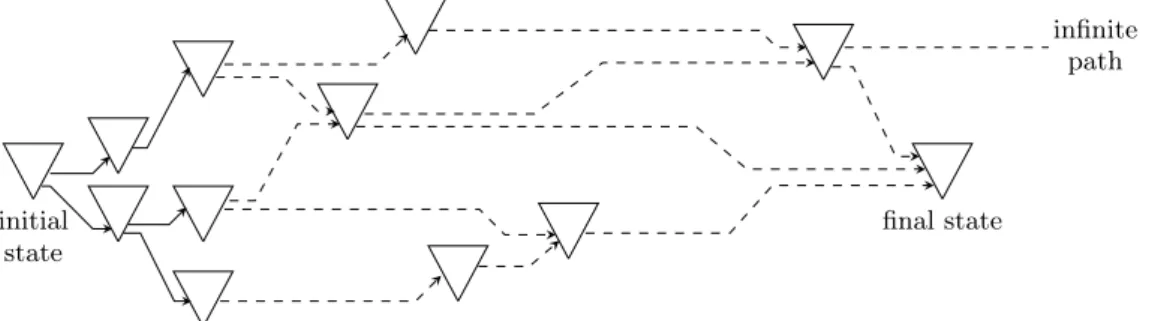
This is one case where starting evaluating the arguments makes the computation non-terminating! initial state infinite path final state
Figure 1.1: Execution Paths (Weak Normalization Case)
In the λ-calculus, a β-normal form is a program such that every computation is in its final state (the program does not contain reducible expressions). One then distin-guishes between weakly normalizing and strongly normalizing λ-terms. A program t is
1.2. PROCESSING COMPUTATION IN FUNCTIONAL PROGRAMMING 25
weakly normalizing when there is at least one reduction path from t to a final state (a β-normal form) whereas it is strongly normalizing when there are no infinite reduction paths starting at t. For instance, the program proj2(expr, 2 + 1) above is weakly, but not strongly, normalizing, whereas the expression f(2 × 3 + 1) from p. 22 corresponds to a strongly normalizing program (it does not even contain “for” or a “while” loop). In Fig. 1.1, we have represented different execution/reduction paths, starting at an initial state/expression of a program. All the paths represented in the figure lead to a final state, except for one. Thus, the program can be executed in some ways that will make it terminate, but some other will not: this roughly corresponds to a case of weak (not strong) normalization in the λ-calculus.
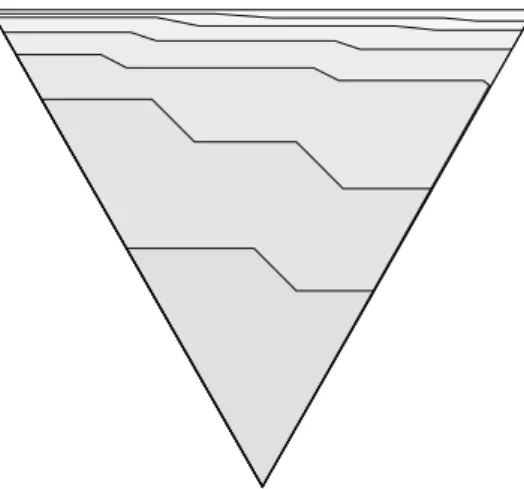
Operational completeness and reduction strategies To get into the subject of reduction strategies, let us give a very high-level representation of a computable func-tional expression expr as a set of computations with nestings. A simple example of nestings is f(2 × 3 + 1) on p. 22: the application of f to 2 × 3 + 1 is the most shallow process (with f : n 7→ (2 + 3) × n × n × n). The sums 2 + 3 and 2 × 3 + 1 are nested in f(2 × 3 + 1) in the expression of f and in its argument respectively. The product 2 × 3 is nested in the sum 2 × 3 + 1. In Fig 1.2, the computations of a given expr are represented by the nodes and the nestings by the edges. Intuitively, these computations are more or less deeply nested in the expression. We consider the computations that do not contain sub-computations10as inputs of the computation (although it is somewhat11of an over-simplification) but there is exactly one computation that is the closest to the output. Every sub-computation of expr has a main process and this main process is either in a final state (we label it with “T”, standing for terminated) or it is not completed – i.e. it can still be reduced – and we label it with “?”.
T T ? ? ? T ? T T ? T
? Most shallow process
Figure 1.2: Dependencies between Computations in a Function
A reduction strategy consists in reducing (executing) only sub-expressions of some particular form or in some particular places e.g., in λ-calculus, the head reduction strategy informally corresponds to keeping on reducing the most shallow process of the expression (the one that is the closest to the output) while it is not in terminal state (the strategy will go on forever if this is not possible).
Still in the λ-calculus, a head normal form is a program whose most shallow process is in terminal state whereas a β-normal form (see above) is a program whose processes are all in final state. One says that a program t is head normalizing if there exist a reduction path (an execution path) from t to a head normal form. Obviously, if the head reduction
10
Computations containing only one operand.
11In general, Fig. 1.2 is far too rudimentary to suitably represent computation dependencies in a
strategy terminates on a program, then it is head normalizing. An equivalence actually holds: a program is head normalizing iff the head reduction strategy terminates on it. We then say that the head reduction strategy is complete for head normalization.
The converse implication of the above equivalence is difficult to prove: the head reduction consists in reducing only the most shallow node i.e. the node of interest, but as we saw on p. 22, each execution-step can displace, duplicate, erase or create new computations. It is sometimes clearly more efficient to reduce first the argument of a computation instead of executing this computation (recall f(2 × 3 + 1) on p. 22) and the head reduction strategy is often quite sub-optimal to reach a head normal form, but still, it ensures that a head normal form will be reached (if one is reachable from the initial state of the program).
Usually, the developer or the user of a program must not be bothered and asked to specify at each execution step which expression should be computed next, and languages feature default deterministic reduction strategies. It is then very useful to identify reduc-tion strategies for given definireduc-tions of terminareduc-tion, so that one ensures that computareduc-tion stops iff a final state is reached. It turns out that intersection type theory provides se-mantic proofs of the operational completeness of a strategy, instead of syntactical ones, and this is one of their main interests.
Reduction Strategies
• For a given program, some execution paths can be infinite whereas some others reach a final state in a finite number of steps.
• A reduction strategy sets priorities of reduction/execution.
• Some reduction strategies are complete w.r.t. some notions of termination.
1.3
Intersection (or not) Types in the λ-Calculus
Type systems, typing derivations The typing of a program roughly consists in a proof, called a typing derivation, following the structure of the instructions of the program. These proofs contain statements called typing judgments and the typing rules of the system describe the licit transitions from one judgment to another. As hinted before, the most important constructor of type theory is the arrow/implication “→”: the judgment f : A → B means that f is a typed function that takes an input of type A and outputs an object of type B.
For instance, if twice is a function computing the double of a natural number (i.e. the type of twice is Nat → Nat) and len computes the length of a string (i.e. the type of len is String → Nat), then the program f defined taking a string s as input and outputting twice(len(s)) should of course be typed with String → int. From the syntactical point of view, this typing is checked like this: under the assumption that s is an object of type String, we prove that twice(len(s)) is a well-defined object of type Nat (this is denoted by the judgment s : String ` twice(len(s)) : Nat: on the left-hand side of `, one finds the typing assumptions). This implies that the function f, defined by s 7→ twice(len(s)), is of type String → Nat. Formally, this corresponds to this typing derivation:
1.3. INTERSECTION (OR NOT) TYPES IN THE λ-CALCULUS 27
` twice : Nat → Nat
` len : String → Nat s : String ` s : String s : String ` len(s) : Nat
s : String ` twice(len(s)) : Nat ` s 7→ twice(len(s)) : String → Nat
In a simple or a higher-order type system, a derivation typing a program featuring 83 functions-calls in its source code will be a proof featuring more or less 83 typing rules/judgments and following the general structure of this source code.
When a type system ensures termination for typed programs, a lot of undecidable problems become decidable e.g., one can usually determine the order of a given typed program by executing it, or decide whether some typed expressions expr1 and expr2 represent states of a same program or not by reducing them.
Types and Termination Revisited As recalled on p. 16, Curry proved in the 50s that typed λ-terms are terminating (they are strongly normalizing), using cut-elimination techniques, and Howard observed that this was just a particular consequence of an iso-morphism between the simply typed λ-calculus and intuitionistic natural deduction. Shortly after, Landin [72,73] used the λ-calculus to construct the language Algol. Curry’s type system does not have much expressive power12and Higher-order types systems, deriving from higher-order deduction systems via the Curry-Howard correspondence, were introduced in the 60s to extend the computational power of the programming languages while ensuring termination of the typed program (see [22], Sec. 8.3 for some historical aspects of higher-order types).
In short, higher-order type systems13 allow manipulating types as first-class objects (one may for instance quantify over types). This approach is embodied by Jean-Yves Girard’ system F [46, 47], Per Martin-Löf type theory [79, 80] and the calculus of constructions (CoC), developed by Thierry Coquand, Gérard Huet and Christine Paulin-Mohring [30–32], and gave birth to a generation of powerful proof assistants like COQ or Agda.
So, why do we need higher order typing? It stems from the observation that, intu-itively, some program can be assigned several different types. For instance, the func-tion app2 from p. 23, satisfying app2(f, x) →β f(f(x)), can be typed with ((Nat → Nat) × Nat) → Nat), since it can take a function f : Nat → Nat as first argument, a natural number n : Nat as second argument, and outputs f(f(n)) which is also of type Nat. In contrast, app2 cannot be typed with (String → Nat × Nat) → Nat because one may not apply a function f of type String → Nat (outputting a number from a string) to a natural number n! But note that app2 can be fed, for any type A, with a function f of type A → A as first input and an argument x of type A as second input, so that app2(f, x) outputs f(f(x)), which is of type A. In other words, f can be typed with ((A → A) × A) → A for all types A. In a higher-order type theory, one then assigns to app2 the type ∀A.((A → A) × A) → A, meaning that the type of app2 may be instantiated so that app2 can be used w.r.t. any “base type” A (e.g., A = Nat as in
12Schwichtenberg [98] proved in 1976 that a function from Nat to Nat can be encoded with a simply
typed λ-term iff it is an extended polynomial i.e. a polynomial using some conditional operator
13this is not to be confused with the fact that the λ-calculus is of higher-order, as a programming
app2(f, n) above, or A = String or A = Nat → Nat). One then says that the type of app2 is polymorphic. Let us give an example of use of this polymorphism:
• Let G be the function that takes a function f : Nat → Nat and outputs the function Nat → Nat defined by n 7→ f (3 × n) + 1. Thus, G is a higher-order function of type (Nat → Nat) → (Nat → Nat). For instance, if f is n 7→ n2, then G(f) is the function n 7→ 9 × n2+ 1.
• Then, if f is a function Nat → Nat, app2(G, f) outputs G(G(f)) i.e. (up to some execution-steps), the function n 7→ f(9 × n) + 2 which is also of type Nat → Nat. In this case, app2 was instantiated with the type A = Nat → Nat and not A = Nat. Thus, app2(app2(G, f), n) outputs (up to some execution-steps) the natural number f(9 × f(9 × n) + 18) + 2. In this expression, app2 occurs twice, but with different types: the type ((Nat → Nat) × Nat) → Nat (case A = Nat) in app2(. . . , n) and the type (((Nat → Nat) → (Nat → Nat)) × (Nat → Nat)) → (Nat → Nat) (case A = Nat → Nat) in app2(G, f). Because of that, in the case of simple typing, the ex-pression app2(app2(G, f), n) would not be typable (one should have chosen the particular type of app2).
Subject Reduction and Invariance of Typing by Execution An important prop-erty, usually verified by simple and higher-order type systems, as the one of the Calculus of Constructions for instance, is subject reduction, which means that a type assign-ment that is valid for the initial state of a program P remains valid for all the states of P during its execution.
For instance, if f is the function n 7→ 3 × n + 1, the program g from Nat to Nat, that takes a natural number n as input and outputs f(n + 2), can be executed in this manner:
g(n) →β f(n + 2) →β 3 × (n + 2) + 1 →β . . . →β 3 × n + 7
The program g passes from its initial state n 7→ f(n + 2) to its final state n 7→ 3 × n + 7 after some execution-steps. Then subject reduction simply ensures that the final ex-pression n 7→ 3 × n + 7 is also a function from Nat to Nat, as the initial one is. This example is somewhat non-plussing because of its straightforwardness, but subject reduc-tion is perhaps the only requirement demanded to every type system. Note that typing is specified by a set of syntactical14 rules, that can be applied to a given expression of a program. Usually, typing features an arrow constructor and f : A → B means that f is a function of type A → B i.e. a function that takes an output of type A and out-puts an object of type B. But beyond that, any constructor (e.g., product, coproduct, intersection, union, higher-order, dependent types, equality types, etc) and any typing rule can be specified without particular restriction, except that if subject reduction15 is not satisfied, the type system will not be meaningful since typing is not invariant under execution as it should be. When a type system satisfies subject reduction, it is said to be (dynamically) sound.
14 In contrast to the realizability approach pioneered by Kleene [68], which is not syntactical but
more semantical.
15i.e. if an expression expr of a given function is typable but not another that is obtained from expr