HAL Id: tel-00128924
https://tel.archives-ouvertes.fr/tel-00128924
Submitted on 5 Feb 2007
HAL is a multi-disciplinary open access
archive for the deposit and dissemination of sci-entific research documents, whether they are pub-lished or not. The documents may come from teaching and research institutions in France or abroad, or from public or private research centers.
L’archive ouverte pluridisciplinaire HAL, est destinée au dépôt et à la diffusion de documents scientifiques de niveau recherche, publiés ou non, émanant des établissements d’enseignement et de recherche français ou étrangers, des laboratoires publics ou privés.
Marc Atlan
To cite this version:
Marc Atlan. Risks, Options on Hedge Funds and Hybrid Products. Mathematics [math]. Université Pierre et Marie Curie - Paris VI, 2007. English. �tel-00128924�
Thèse de doctorat de l’Université Paris VI
Spécialité : Mathématiques
Présentée par Marc ATLAN
pour obtenir le grade de Docteur de l’Université Paris VI
Sujet de la thèse :
Risques, Options sur Hedge Funds et Produits
Hybrides
Soutenue le 23 Janvier 2007, devant le jury composé de :
Mme Hélyette GEMAN (ESSEC - Birkbeck College), co-directrice de thèse Mme Monique JEANBLANC (Université d’Evry), rapporteur
M. Damien LAMBERTON (Université de Marne-la-Vallée), rapporteur M. Dilip MADAN (University of Maryland), examinateur
M. Gilles PAGÈS (Université Paris VI), examinateur M. Marc YOR (Université Paris VI), directeur de thèse
Remerciements
Je tiens tout d’abord à exprimer toute ma gratitude au professeur Marc Yor pour tout ce qu’il m’a apporté ces quatre dernières années que je ne pourrais résumer en ces quelques lignes. Je vous remercie en premier lieu pour m’avoir enseigné l’indépendance, le goût de la recherche et en second lieu pour votre enthousiasme, votre disponibilité, votre connaissance et tous vos conseils qui m’ont permis ainsi de découvrir tant de choses et de mûrir dans mon appréhension des problèmes. Je vous remercie ensuite pour m’avoir laissé libre dans mes choix de sujets de recherche et dans mes méthodes de travail. Je vous remercie enfin pour m’avoir offert le privilège de participer à votre groupe de travail avec Hélyette Geman et Dilip Madan durant toutes ces années de thèse et par la même occasion pour me les avoir présentés.
Je remercie très sincèrement le professeur Hélyette Geman pour tout ce qu’elle m’a enseigné, son soutien, son amitié, sa connaissance et tous ses conseils avisés tout au long de ces années à Paris ainsi que pendant mes séjours à Londres, New York et Tokyo.
I would like to thank as well the professor Dilip Madan for all the knowledge he has taught me over the past few years, for having constantly given me the taste for research when I was living in New York and for having introduced me to the mathematical finance community in the United States.
Je suis très reconnaissant à Monique Jeanblanc et Damien Lamberton d’avoir accepté d’être rapporteurs de ce travail. Cela me fait tout particulièrement plaisir que Damien Lamberton soit membre de ce jury car c’est au travers de son livre coécrit avec Bernard Lapeyre que j’ai décidé de m’orienter vers les probabilités alors que j’étais encore en classes préparatoires. Je suis également très honoré de la participation de Gilles Pagès au jury de cette thèse que je remercie également pour les discussions que nous avons pu avoir.
Je remercie Boris Leblanc avec qui j’ai écrit deux articles et eu le privilège de travailler sur un grand nombre de problèmes quand j’étais accueilli à la BNP. Je remercie également Stéphane Tyc pour m’avoir accueilli dans son équipe, m’avoir aidé et conseillé à maintes reprises et laissé la liberté d’aborder des sujets variés.
J’aimerais aussi exprimer ma reconnaissance à toute l’équipe administrative du laboratoire, Jo-sette Saman, Nelly Lecquyer, Philippe Macé et Jacques Portes, pour leur gentillesse, disponibilité et compétence.
Merci également à tous les thésards du laboratoire pour leur solidarité et les discussions diverses. Je remercie en particulier Ashkan, Jan, Joseph, Roger et Sacha.
J’aimerais également exprimer toute ma reconnaissance à Nathanaël Enriquez pour les discus-sions mathématiques, le soutien et les conseils éclairés.
Merci à mes amis proches, Jean-François, Jean-Samuel, Julien, Laurent, Raphaël, Pierre et Sté-phane pour avoir été à mes côtés dans les moments difficiles et pour m’avoir constamment encouragé.
Merci à ma soeur Caroline pour ses encouragements.
Enfin, je voudrais remercier mes parents et leur exprimer mon infinie gratitude, pour tout ce qu’ils m’ont apporté durant ma thèse et au cours de toutes les années précédentes.
Table des matières
Introduction vii
0.1 Motivations . . . vii
0.2 Organisation et contribution . . . vii
0.3 Les contributions nouvelles . . . viii
0.3.1 Autour de la Volatilité Locale . . . viii
0.3.2 Valorisation de Produits Dérivés Hybrides Action et Crédit . . . ix
0.3.3 Frais de gestion et de performance et Options sur Hedge Funds . . . x
0.3.4 Prime de Risque et Théorie Générale des Processus . . . xi
1 Localizing Volatilities 1 1.1 Introduction . . . 1
1.2 Preliminary Mathematical Results . . . 2
1.2.1 Bessel and CIR Processes . . . 2
1.2.2 Mimicking Theorems . . . 4
1.3 Generalities on Local Volatility . . . 7
1.3.1 Fokker-Planck Equation . . . 7
1.3.2 Matching Local and Stochastic Volatilities . . . 7
1.4 Applications to the Heston (1993) model and Extensions . . . 9
1.4.1 The Simplest Heston Model . . . 9
1.4.2 Adding the Correlation . . . 13
1.4.3 From a Bessel Volatility process to the Heston Model . . . 15
1.5 Pricing Equity Derivatives under Stochastic Interest Rates . . . 17
1.5.1 A Local Volatility Framework . . . 17
1.5.2 Mimicking Stochastic Volatility Models . . . 18
1.5.3 From a Deterministic Interest Rates Framework to a Stochastic one . . . 20
1.6 Conclusion . . . 23
2 Time-Changed Bessel Processes and Credit Risk 29 2.1 Introduction . . . 29
2.2 A Mathematical Study of CEV Processes . . . 31
2.2.1 Space and Time Transformations . . . 31
2.2.2 Distributions and Boundaries . . . 32
2.2.3 Loss of Martingality . . . 36
2.3 Credit-Equity Modelling . . . 38 iii
2.3.1 Model Implementation . . . 38
2.3.2 European Vanilla Option Pricing . . . 39
2.3.3 Pricing of Credit and Equity Default Swaps . . . 40
2.4 Stochastic Volatility for CEV Processes . . . 41
2.4.1 A Zero Correlation Pricing Framework . . . 41
2.4.2 CESV Models . . . 44
2.4.3 Subordinated Bessel Models . . . 48
2.5 Correlation Adjustment . . . 50
2.5.1 Introducing some Correlation . . . 50
2.5.2 Pricing Credit and Equity Derivatives . . . 51
2.5.3 Examples . . . 52
2.6 Conclusion . . . 55
3 Hybrid Equity-Credit Modelling 61 3.1 Introduction . . . 61
3.2 Tracking a Stock Price Process that models default . . . 62
3.2.1 Poisson Default Models . . . 63
3.2.2 CEV Diffusion . . . 63
3.2.3 Poisson Default Process Problem . . . 64
3.3 Consistent Pricing of Credit and Equity Derivatives within CEV . . . 65
3.3.1 Calibration and Pricing of Vanilla Options . . . 65
3.3.2 Credit Derivatives Pricing . . . 68
3.4 Heston CESV Model . . . 69
3.5 Conclusion . . . 72
4 Options on Hedge Funds under the High-Water Mark Rule 77 4.1 Introduction . . . 77
4.2 The High-Water Mark Rule and Local Times . . . 78
4.2.1 Modeling the High-Water Mark . . . 78
4.2.2 Building the Pricing Framework . . . 81
4.2.3 Valuation of the Option at Inception of the Contract . . . 83
4.2.4 Valuation during the lifetime of the Option . . . 85
4.2.5 Extension to a Moving High-Water Mark . . . 90
4.3 Numerical Approaches to the NAV option prices . . . 92
4.4 Conclusion . . . 95
4.5 Appendix : Excursion Theory . . . 96
5 Correlation and the Pricing of Risks 99 5.1 Introduction . . . 99
5.2 Financial Commentary . . . 102
5.2.1 Catastrophic Risk and Measure Changes . . . 103
5.2.2 Self Sufficiency in the Heston Model . . . 103
5.2.3 Dependence and No change of Measure . . . 103
5.3 Single Period Risk . . . 103
Table des matières v
5.4.1 The Examples . . . 113
5.4.2 Almost No Kernel Pricing for filtrations . . . 121
5.4.3 ANKP for filtrations and the examples . . . 123
5.4.4 A decomposition of risks . . . 123
5.5 Self Sufficiency and Measure Changes . . . 124
5.6 Event Risk and No Kernel Price . . . 128
Introduction
0.1
Motivations
Cette thèse a deux objectifs principaux :
-Le premier est d’aborder des problèmes de modélisation liés à l’émergence de nouveaux types de produits dérivés. Ainsi, des questions telles que la dépendance entre le marché Actions et celui du Crédit ou celle entre le marché Actions et celui des Taux d’intérêt sont étudiées. La prise en compte de la nature spécifique des frais de gestion facturés par les hedge funds à leurs investisseurs est modélisée afin d’évaluer cet effet dans le pricing d’options sur les hedge funds eux-mêmes. Les différentes modélisations ainsi obtenues m’ont conduit à étudier la littérature sur les distributions des processus de Bessel et de diffusions qui en dérivent, la théorie des excursions du mouvement Brownien, les premiers temps de passage de ces processus, la théorie des changements de temps et les concepts de vraie martingale et/ou martingale locale stricte.
-Le second objectif est de s’interroger sur la notion de prime de risque sur les marchés d’options en faisant abstraction des modèles mathématiques sous-jacents. Pour cela, la théorie générale des processus et plus particulièrement les concepts d’immersion et de changement de mesure devraient permettre aux agents financiers de comprendre les risques non ou mal perçus par les modélisations usuelles.
0.2
Organisation et contribution
• Cette thèse est composée de cinq chapitres qui correspondent aux articles écrits entre Janvier 2004 et Avril 2006. Chaque chapitre peut, en principe, être lu indépendamment des autres. Toutefois, à bien des égards, les trois premiers chapitres se complètent. Tout d’abord, ils traitent tous les trois de problèmes liés aux modèles hybrides, ensuite ils utilisent des propriétés des processus de Bessel et enfin ils abordent des questions de volatilité locale, de volatilité stochastique ainsi que de volatilité locale stochastique. Sur la question des hybrides, le premier chapitre aborde l’impact de taux d’intérêt stochastiques sur l’évaluation d’options sur actions alors que les chapitres 2 et 3 (écrits avec Boris Leblanc) étudient la dépendance entre le marché des actions et celui du crédit. Enfin, ils visent à fournir des formules analytiques pour les différentes quantités mises en jeu ; nous reviendrons sur celles-ci dans les chapitres concernés ainsi que brièvement dans la section qui suit.
• Le chapitre 4 (écrit avec Hélyette Geman et Marc Yor), quant à lui, propose un modèle stochastique où l’actif étudié est un hedge fund et où l’on tient compte des frais de gestion et de performance. Il y est choisi un modèle de type Brownien géométrique ou encore de type Black Merton Scholes (1973) et l’on considère un drift qui est une fonction déterministe du temps et de
la Valeur Actualisée Net (NAV) du fond. Dans ce contexte, nous sommes en mesure de fournir des formules quasi-analytiques pour des prix d’options vanille européennes. Le modèle ainsi construit est finalement une diffusion à volatilité constante mais à drift local où la forme particulière du drift permet d’obtenir une formule fermée pour la transformée de Laplace de la loi de la NAV. Il apparaît ainsi que mathématiquement les quatre premiers chapitres ont en commun l’étude de diffusions inhomogènes dont les dynamiques, telles qu’elles sont spécifiées, en font des modèles intéressants et nouveaux en mathématiques financières.
• Pour résumer la démarche suivie dans cette thèse, des produits nouveaux y sont étudiés et des risques généralement ignorés dans les modélisations classiques y sont caractérisés. Ceci peut être compris comme une illustration du principe d’adaptation de modèles connus à des problèmes nouveaux. Ayant choisi d’observer les modèles d’évaluation sous l’angle des risques qui sont pris en compte, l’on est naturellement amené à se demander ce que signifie valoriser un risque. Ceci nous ramène à l’idée de Markowitz (1952) qui formalise le fait qu’un risque est valorisé dès lors qu’il y a un excès de rendement. Dans le langage probabiliste des options, cela veut dire que la mesure de pricing sous la probabilité statistique et celle sous la probabilité risque-neutre diffèrent.
• Ainsi, le chapitre 5 écrit avec Hélyette Geman, Dilip Madan et Marc Yor examine à un niveau conceptuel illustré d’exemples provenant de propriétés fines du mouvement Brownien et des grossissements de filtration, la question des risques qui sont ou ne sont pas pricés dans une économie. On introduit diverses acceptions pour la notion de risque valorisé dans le chapitre 5.
0.3
Les contributions nouvelles
Dans les quatre paragraphes ci-dessous, nous donnons les idées maîtresses et les principaux résultats des cinq chapitres (le second paragraphe regroupe la discussion sur les chapitres 2 et 3) qui composent cette thèse.
0.3.1 Autour de la Volatilité Locale
Il s’agit ici de présenter succinctement les principales directions du chapitre 1 qui est en fait un article intitulé Localizing volatilities. Rappelons d’abord que le concept de volatilité locale remonte à Dupire (1994) et Derman et Kani (1994) et que si l’on considère un actif modélisé par la diffusion :
dSt
St
= r(t)dt + σ(t, St)dWt
alors connaissant les prix des calls pour un continuum de maturités et de prix d’exercice, la fonction (t, x) 7→ σ(t, x) peut être définie implicitement par
σ2(t, x) = ∂C ∂t + xr(t)∂C∂x 1 2x2 ∂ 2C ∂x2
A présent, considérons un modèle à volatilité stochastique générale de la forme dSt
St
0.3. Les contributions nouvelles ix où σtest un processus d’Itô continu. En se fondant sur les résultats de Gyöngy (1986), l’on obtient
l’existence d’une équation différentielle stochastique Markovienne inhomogène telle que, à t fixé, la loi de la solution soit exactement la même que celle de St. De plus, on est capable de construire
cette EDS et l’on obtient ainsi une détermination de la fonction σ(t, x) : σ2(t, x) = E[σ2t|St= x]
Maintenant qu’il est établi comment les modèles à volatilité stochastique et volatilité locale sont liés, l’on fournit une série d’exemples de modèles à volatilité stochastique construits à partir de processus de Bessel (type Heston (1993)) où l’on est en mesure de calculer explicitement la fonction volatilité locale. Le calcul de la volatilité locale est alors principalement basé sur la connaissance de la loi du couple (R2t, At) où (Rt, t ≥ 0) est un processus de Bessel et At=R0tR2sds.
L’autre direction principale de ce chapitre est l’addition de taux d’intérêt stochastiques à la diffusion à laquelle le cours de l’actif obéit. Ainsi, la dynamique de l’action s’écrit :
dSt
St
= rtdt + σtdWt
où (rt, t ≥ 0) est également un processus d’Itô continu. Nous étendons les résultats connus dans le
cas de taux déterministes et obtenons l’existence d’une diffusion de la forme : dXt
Xt
= rtdt + σ(t, Xt)dWt
telle que pour tout t fixé, les lois de St et Xt soient les mêmes. Pour cela, la fonction σ(t, x) doit
vérifier : σ2(t, x) = E[σ 2 te− Rt 0rsds|St= x] E[e−R0trsds|St= x]
D’autre part, l’équation implicite portant sur la volatilité locale peut être étendue au cas des taux stochastiques de la façon suivante :
σ2(t, x) = ∂C ∂t − xE[e− Rt 0rsdsr t1{St>x}] x2 2 ∂ 2C ∂x2
D’autres constructions de volatilité locale à partir de modèles à volatilité stochastique sont proposées dans ce chapitre et une réécriture et discussion de l’équation implicite ci-dessus sont fournies.
0.3.2 Valorisation de Produits Dérivés Hybrides Action et Crédit
Cette section résume le travail élaboré en collaboration avec Boris Leblanc qui a donné lieu à deux chapitres (2 et 3) de cette thèse et ainsi qu’à deux articles dont le premier intitulé Time-Changed Bessel Processes and Credit Risk est soumis à Mathematical Finance et dont le second intitulé Hybrid Equity-Credit Modelling a été publié dans Risk Magazine. La problématique posée est la modélisation du cours de l’action d’une compagnie en tenant compte de son risque de faillite,
lui-même un actif financier coté sur le marché obligataire et sur celui du crédit. Un standard de marché depuis quelques années pour modéliser le cours d’une action sous cette contrainte est le modèle à probabilité locale de défaut (voir par exemple Davis et Lischka (2002)) où le défaut que l’on définit comme le fait que l’action vaille zéro, est calibré sur un processus à sauts destiné à engendrer la faillite et dont la partie continue est quant à elle présente pour calibrer la surface de volatilité implicite dans des zones où les options sont cotées.
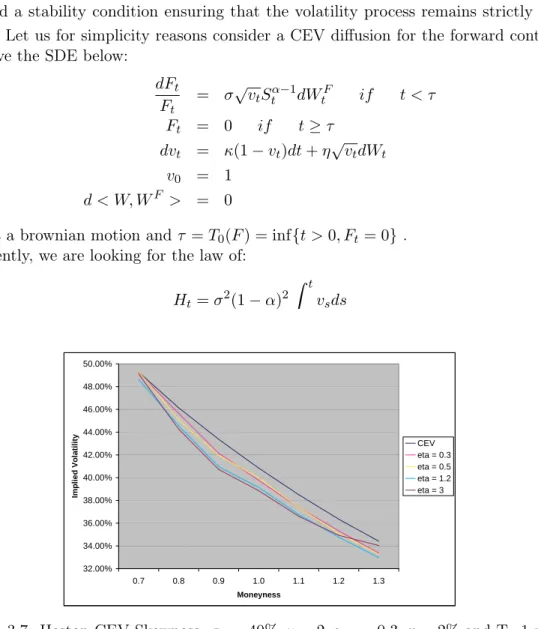
Le problème de ce type de modélisation est qu’il ne tient pas compte des scénarios de marché où le cours de l’actif baisse lentement en se dirigeant vers la faillite sans pour autant faire de saut significatif et en entraînant une hausse des spreads de crédit. Ayant ce type d’inconvénient à l’esprit, nous nous intéressons au modèle Constant Elasticity of Variance de Cox (1975) pour son aptitude à générer des trajectoires qui atteignent 0 en un temps fini. Cette propriété résulte du fait que le CEV peut être vu comme une puissance de Bessel changé de temps. On notera que dans la même année Albanese et Chen (2005), Campi, Polbennikov et Sbuelz (2005) et Carr et Linetsky (2005) ont étudié ce modèle dans le même objectif. Rappelons maintenant la dynamique de ce processus :
dSt
St
= rdt + σStα−1dWt
Ainsi le chapitre 2 propose une étude détaillée du processus CEV ; on y appliquera les résultats de cette étude à la valorisation d’options vanilles, de credit default swaps (CDS) et d’equity default swaps (EDS) pour lesquels on obtient des formules analytiques. L’on étend par la suite ce modèle en y ajoutant une volatilité stochastique dont le mouvement brownien qui l’engendre est supposé indépendant de celui qui engendre le cours de l’action :
dSt
St
= rdt + σtStα−1dWt
Dans cette configuration, l’on est en mesure d’obtenir des formules analytiques pour les prix d’op-tions et pour les CDS conditionnellement à la connaissance de la loi pour tout t de la quantité
Ht= (1 − α)2
Z t 0
σ2se−2(1−α)rsds
L’addition de volatilité stochastique permet de générer plus ou moins de skew et de smile à la surface de volatilité implicite. Maintenant afin de pouvoir décorréler la probabilité de défaut de la "skewness", on corrèle les mouvements de l’action à ceux de sa volatilité. De nombreux exemples où des calculs analytiques sont possibles sont présentés.
Le chapitre 3 illustre de façon appliquée ces propriétés mathématiques des processus CEV et im-plicitement des processus de Bessel, et également les arguments financiers empiriques discutés plus haut et qui y sont détaillés.
0.3.3 Frais de gestion et de performance et Options sur Hedge Funds
Lors de l’évaluation d’options sur Hedge Funds, sous réserve que l’on puisse se couvrir, il est important de considérer les différents frais (importants) liés à la détention de participations dans un hedge fund. En effet, l’investisseur est soumis à des frais de gestion qui sont fixes et de l’ordre de 1% à 2% du montant investi mais il est également soumis à des frais de performance suivant la High-Water Mark rule, qui sont de l’ordre de 15% à 20% de la performance annuelle du hedge
0.3. Les contributions nouvelles xi fund. Cette question est traitée dans le chapitre 4 qui, à l’origine, est un article écrit avec Hélyette Geman et Marc Yor intitulé Options on Hedge Funds under the High-Water Mark Rule soumis à Quantitative Finance.
Afin de tenir compte de ces différents frais, nous proposons le modèle suivant pour régir la valeur nette actualisée S :
dSt
St = (r + α − c − f(St
))dt + σdWt
où r est le taux sans risque, c représente les frais de gestion, α l’excès de rendement du fond par rapport au marché, f est la fonction modélisant le high-water mark :
f (s) = µa 1{s>H}
et µ est le rendement statistiquement observé, a le pourcentage prélevé sur la performance et H le niveau par rapport auquel cette performance est mesurée.
Relativement à ce modèle, nous sommes en mesure de calculer les prix de calls européens. Ainsi, l’on démontre que le calcul des prix d’options vanille repose essentiellement sur la connaissance de la quantité
g(t) = E£h(Wt) exp(λLt) exp(−µA+t − νA−t)
¤
où Wt est un mouvement brownien, Lt est son temps local en 0 et A+t etA−t respectivement les
temps passés positivement et négativement jusqu’au temps t. Il est remarquable que la variable tri-dimensionnelle mise en jeu (Wt, Lt, A+t ) joue un rôle crucial dans l’étude de la loi de l’Arcsinus
étudié par exemple dans Karatzas et Shreve (1991). Il est relativement clair que le calcul de la transformée de Laplace de g peut être fait, par exemple, via un détour par la théorie des excursions du mouvement brownien (voir Jeanblanc, Pitman et Yor (1997) ou Revuz et Yor (2005)) et l’on démontre ainsi que pour tout θ suffisamment grand
Z ∞ 0 dte−θ2tg(t) = 2 µR ∞ 0 dxe−x √ θ+2µh(x) +R∞ 0 dxe−x √ θ+2νh(−x) ¶ √ θ + 2µ +√θ + 2ν − 2λ
0.3.4 Prime de Risque et Théorie Générale des Processus
Une question très importante en finance de marché est l’identification des risques dans l’évalua-tion d’actifs financiers. Depuis Fama (1970), l’on dit qu’un risque est valorisé dans l’évalual’évalua-tion d’un actif financier dès lors que la covariance entre le risque considéré et l’actif observé est différente de zéro. Une conséquence importante de cette vision est qu’un risque n’est pas valorisé dans une éco-nomie s’il n’est pas corrélé aux actifs qui la composent. Un peu plus récemment dans la littérature sur les produits dérivés (Harrison et Kreps (1979), Harrison et Pliska (1981)), un risque est pricé si les valorisations de l’actif d’Arrow Debreu associé à ce risque ont des espérances différentes sous la probabilité statistique et sous la probabilité risque neutre. Les deux approches sont cohérentes dans la mesure où un risque est pricé dès qu’il impacte les excès de rendements. Mathématiquement, la corrélation entre les processus de l’économie et le risque donné précisément par le changement de
mesure n’est pas un critère suffisant pour assurer qu’un risque est pricé ou non.
Selon ces considérations, le chapitre 5 rédigé avec Hélyette Geman, Dilip Madan et Marc Yor a donné lieu à un article intitulé Correlation and the Pricing of Risks accepté dans Annals of Finance. Nous y fournissons entre autres des exemples de risques pricés et de corrélation nulle. Après l’introduction de nouveaux concepts et une étude détaillée de la notion de risque, laquelle est considéré aussi bien au niveau des variables aléatoires, des processus continus que des filtrations nous sommes capables de montrer que l’absence d’excès de rendement et une corrélation nulle pour des processus continus sont équivalents à condition de se placer dans une filtration étendue que l’on appellera self sufficient. Cette filtration construite en détail dans le chapitre 5 prend en compte les trajectoires de processus permettant de prédire l’évolution du risque considéré. Nous démontrons que la self sufficiency d’une filtration dépend de la mesure de probabilité sous laquelle elle est étudiée et nous examinons les changements de mesure de probabilité pour lesquelles la self sufficiency est préservée.
Bibliographie
[1] Albanese, C. and O. Chen (2005), “Pricing Equity Default Swaps,” Risk, 6, 83-87.
[2] Black F. and M. Scholes (1973), “The Pricing of Options and Corporate Liabilities,” Journal of Political Economy, 81, 637-654.
[3] Campi, L., S. Polbennikov and A. Sbuelz (2005), “Assessing Credit with Equity : A CEV Model with Jump to Default,” Working Paper.
[4] Carr, P. and V. Linetsky (2005), “A Jump to Default Extended CEV Model : An Application of Bessel Processes,” Working Paper
[5] Cox, D. (1975), “Notes on Option Pricing I : Constant Elasticity of Variance Diffusions,” Stan-ford University, Graduate School of Business.
[6] Davis, M., and F. Lischka (2002), “Convertible bonds with market risk and credit risk,” In Applied Probability, Studies in Advanced Mathematics, American Mathematical So-ciety/International Press, 45-58.
[7] Derman, E. and I. Kani (1994), “Riding on a Smile,” Risk, 7, 32-39. [8] Dupire, B. (1994), “Pricing with a smile,” Risk, 7, 18-20.
[9] Fama, E.F. (1970), “Efficient Capital Markets : A Review of Theory and Empirical Work,” Journal of Finance, 383-417.
[10] Gyöngy, I. (1986), “Mimicking the One-Dimensional Marginal Distributions of Processes Having an Ito Differential,” Probability Theory and Related Fields, 71, 501-516.
[11] Harrison, J.M. and D. Kreps (1979), “Martingales and Arbitrage in Multiperiod Securities Markets,” Journal of Economic Theory, 20, 381-408.
[12] Harrison, J.M. and S. Pliska (1981), “Martingales and Stochastic Integrals in the Theory of Continuous Trading,” Stochastic Processes and Their Applications, 15, 215-260.
[13] Heston, S. (1993), “A closed-form solution for options with stochastic volatility with applications to bond and currency options.” Review of Financial Studies, 6, 327-343.
[14] Jeanblanc, M., J. Pitman and M. Yor (1997), “Feynman-Kac formula and decompositions of Brownian paths,” Computational and applied Mathematics, 16, 27-52, Birkhäuser.
[15] Karatzas, I. and S.E. Shreve (1991), Brownian Motion and Stochastic Calculus, Second Edition, Springer-Verlag, New York.
[16] Markowitz, H. (1952), “Porfolio Selection, ” Journal of Finance, 7, 77-91.
[17] Merton, R.C. (1973), “Theory of Rational Option Pricing, ” Bell Journal of Economics and Management Science, 4, 141-183.
[18] Revuz, D. and M. Yor (2005), Continuous Martingales and Brownian Motion, Third Edition, Springer-Verlag, Berlin.
Chapitre 1
Localizing Volatilities
[Submitted∗]
We propose two main applications of Gyöngy (1986)’s construction of inhomogeneous Markov-ian stochastic differential equations that mimick the one-dimensional marginals of continuous Itô processes. Firstly, we prove Dupire (1994) and Derman and Kani (1994)’s result. We then present Bessel-based stochastic volatility models in which this relation is used to compute analytical formu-las for the local volatility. Secondly, we use these mimicking techniques to extend the well-known local volatility results to a stochastic interest rates framework.
1.1
Introduction
It has been widely accepted for at least a decade that the option pricing theory of Black and Scholes (1973) and Merton (1973) has been inconsistent with option prices. Actually, the model implies that the informational content of the option surface is one dimensional which means that one could construct the prices of options at all strikes and maturities from the price of any single option. It has also been shown that unconditional returns show excess kurtosis and skewness which are inconsistent with normality. Special attention was given to implied volatility smile or skew, but research has concentrated on implied Black and Scholes volatility since it has become the unique way to price vanilla options. Accordingly, option prices are often quoted by their implied volatility. Nevertheless, this method is unsuitable for more complicated exotic options and options with early exercise features. To explain in a self-consistent way why options with different strikes and maturi-ties have different implied volatilimaturi-ties or what one calls the volatility smile, one could use stochastic volatility models (eg. Heston (1993) or Hull and White (1987))
Given the computational complexity of stochastic volatility models and the difficulty of fitting their parameters to the market prices of vanilla options, practitioners found a simpler way to price exotic options consistently with the volatility smile by using local volatility models as introduced by Dupire (1994) and Derman and Kani (1994). Local volatility models have the advantage to fit the implied volatility surface; hence, when pricing an exotic option, one feels comfortable hedging
∗I thank Marc Yor for providing key ideas for the elaboration of this work and for all his precious comments. I
also thank Hélyette Geman for all her helpful and useful remarks. 1
through the stock and vanilla options markets.
In the last twenty years, academics and practitioners have been primarily interested in building models that describe well the behavior of an asset whether it is equity, FX, Credit, Fixed-Income or Commodities and very rarely models that specify any cross-asset dependency. For all cross-asset derivative products, this dependency modifies the model one should use or at least the calibration procedure. Certainly, models that incorporate a dependency on other asset classes than a specific underlying need to be recalibrated as soon as the other asset classes become random, in particular in the fast growing hybrid industry where it is necessary to model several assets.
The remainder of the paper is organized as follows. Section 2 recalls preliminary results on Bessel processes and states mimicking properties of continuous Itô processes exhibited by Gyöngy (1986) and Krylov (1985). Section 3 recalls well-known results of Dupire (1994) and Derman and Kani (1994) on local volatility, gives a proof of the existence of a local volatility model that mimicks a stochastic volatility one based on Gyöngy (1986) theorem. Section 4 gives examples of stochastic volatility models where a local volatility can be computed. Those examples are based on remarkable properties of Bessel processes such as scaling properties. In order to extend the class of volatility models (where closed-form formulas can be obtained), we propose a general framework in which the volatility diffusion is a general deterministic time and space transformation of Bessel processes. Analytical computations are proposed in cases where the volatility diffusion is independent from the stock price diffusion as well as in cases where they are correlated. Section 5 applies the results of Section 3 to the case of stochastic interest rates and more generally shows how Gyöngy (1986) theorem can be applied to construct a local volatility model in a deterministic interest rate frame-work, starting from a stochastic volatility model with stochastic rates. Finally, Section 6 concludes our work and presents an important open question on mimicking the laws of Itô processes.
1.2
Preliminary Mathematical Results
1.2.1 Bessel and CIR Processes
Let (Rt, t ≥ 0) denote a Bessel process with dimension δ, starting from 0 and (βt, t ≥ 0) an
independent brownian motion from (Bt, t ≥ 0) the driving brownian motion. Let us recall that R2t
solves the following SDE:
dR2t = 2RtdBt+ δdt
and let us now define :
It= Z t 0 Rsdβs and At= Z t 0 Rs2ds
Then, the one-dimensional marginals of (At, It) are at least in theory well-identified, via
Fourier-Laplace expressions, and are closely related with the so-called Lévy area formula (see Lévy (1950), Williams (1976), Gaveau (1977), Yor (1980), Chapter 2 of Yor (1992) and many other references). Here we simply recall, for our purposes the formulae:
∀(α, β) ∈ R2 E · exp¡iαIt− β2 2 At ¢¸ =¡cosh(tpα2+ β2)¢−δ2 (1.1)
1.2. Preliminary Mathematical Results 3 as well as: ∀(a, b) ∈ R+× R E · exp¡− aR2t −b 2 2At ¢¸ =¡cosh(bt) +2a b sinh(bt) ¢−δ 2 (1.2)
a formula that we shall use later. Some developments for the law of At are given, e.g. in Pitman
and Yor (2003).
For a Bessel process of dimension δ starting at x, one gets the following formula: ∀(a, b) ∈ R+× R Ex · exp¡− aR2t −b 2 2At ¢¸ =¡cosh(bt) +2a b sinh(bt) ¢−δ 2 × exp µ −x 2b 2 sinh(bt) +2ab cosh(bt) cosh(bt) +2ab sinh(bt) 
Let us now present a scaling property of the Bessel process with respect to conditioning, which is important in the sequel.
Proposition 1.2.1 For any Bessel process Rt with dimension δ, we have:
E · R2t| Z t 0 R2sds ¸ = 2 t Z t 0 R2sds (1.3)
Remark 1.2.2 This result is in fact a very particular case of a more general result involving only the scaling property of the process (R2
t, t ≥ 0), see, e.g, Pitman and Yor (2003). But, for the sake
of completeness, we shall give a direct proof of (1.3) below:
Proof. From the scaling property of (R2t, t ≥ 0), we deduce that for every f ∈ C1(R, R+), with
bounded derivative, we have: E · f µ Z t 0 R2sds ¶¸ = E · f µ t2 Z 1 0 R2sds ¶¸
We then differentiate both sides with respect to t, to obtain: E · f′ µ Z t 0 R2sds ¶ Rt2 ¸ = E · f′ µ t2 Z 1 0 R2sds ¶ (2t) Z 1 0 Rs2ds ¸ = E · f′ µ Z t 0 R2sds ¶ 2 t Z t 0 R2sds ¸
Since this identity is true for every bounded Borel function f′, the identity (1.3) follows.
Remark 1.2.3 We now check that formula (1.3) can be obtained directly as a consequence of for-mula (1.2): differentiating (1.2) both sides with respect to a and taking a = 0, we obtain:
E · R2texp¡−b 2 2At ¢¸ = δ (cosh(bt))δ2+1 ¡1 b sinh(bt) ¢
while, taking a = 0 in (1.2), and differentiating both sides with respect to b, we get: bE · Atexp¡− b2 2At ¢¸ = δt 2(cosh(bt))2δ+1 sinh(bt)
and the identity (1.2) follows from the comparison of these last two equations.
A reason why squared Bessel processes play an important role in financial mathematics is that they are connected to models used in finance. One of these models is the Cox, Ingersoll and Ross (1985) CIR family of diffusions which are solutions of the following kind of SDEs:
dXt= (a − bXt)dt + σ
p
|Xt|dWt (1.4)
with X0 = x0 > 0, a ∈ R+, b ∈ R, σ > 0 and Wt a standard brownian motion. This equation
admits a unique strong (that is to say adapted to the natural filtration of Wt) solution that takes
values in R+.
One is now interested in the representation of a CIR process in terms of a time-space transfor-mation of a Bessel process:
Lemma 1.2.4 A CIR Process Xt solution of equation (2.1) can be represented in the following
form:
Xt= e−btR2σ2 4b(ebt−1)
(1.5) where R denotes a Bessel process starting from x0 at time t = 0 of dimension δ = 4aσ2
Proof. This lemma results from simple properties of squared Bessel processes that can be found in Revuz and Yor (2001), Pitman and Yor (1980, 1982).
This relation has been widely used in finance, for instance in Geman and Yor (1993) or Delbaen and Shirakawa (1996).
1.2.2 Mimicking Theorems
A common topic of interest of Krylov and Gyöngy respectively in Krylov (1985) and Gyöngy (1986) is the construction of stochastic differential equations whose solutions mimick certain features of the solutions of Itô processes. The construction of Markov martingales that have specified marginals was studied by Madan and Yor (2002). Bibby, Skovgaard and Sørensen (2005) as well as Bibby and Sørensen (1995) proposed construction of diffusion-type models with given marginals.
Let us now consider an Itô differential equation of the form: ξt= Z t 0 δsdWs+ Z t 0 βsds (1.6)
where Wt is a Ft-Brownian motion of dimension k, (δt)t∈R+ and (βt)t∈R+ are bounded Ft-adapted
1.2. Preliminary Mathematical Results 5 Definition 1.2.5 (Green Measure) Considering two stochastic processes Xt, valued in Rn and
γt, with γt> 0, one defines the Green measure µX,γ by:
µX,γ(Γ) = E · Z ∞ 0 1Γ(Xt) exp¡− Z t 0 γsds¢dt ¸ (1.7) where Γ is any borel set of Rn
Remark 1.2.6 The stochastic process γt is called the killing rate
Theorem 1.2.7 (Krylov) If ξt is an Itô process defined as previously and satisfying the uniform
ellipticity condition: ∃λ ∈ R∗
+ such as δδ∗≥ λIn
as well as the lower boundedness condition: ∃α ∈ R+ such as γ > α,
then there exist deterministic functions σ : Rn→ Mn(R) , b : Rn→ Rn and c : Rn→ R+ such that
the following SDE:
dxt = σ(xt)dWt+ b(xt)dt
x0 = 0
has a weak solution satisfying:
∀Γ ∈ B(Rn) E · Z ∞ 0 1Γ(ξt) exp¡− Z t 0 γsds¢dt ¸ = E · Z ∞ 0 1Γ(xt) exp¡− Z t 0 c(xs)ds¢dt ¸ ie : µξ,γ(Γ) = µX,c(Γ)
Proof. See Krylov (1985)
Definition 1.2.8 (Weak Solution) The stochastic differential equation
dXt = f (t, Xt)dWt+ g(t, Xt)dt (1.8)
X0 = 0 (1.9)
is said to have a weak solution if there exist a probability space (Ω, F, P) and an Ft-Brownian motion
with respect to which there exists a Ft-adapted stochastic process Xt that satisfies (1.8) and (1.9).
A natural question asked and answered by Gyöngy is whether it is possible to find the solution of an SDE with the same one-dimensional marginal distributions as an Itô process. The answer is stated below:
Theorem 1.2.9 (Gyöngy) If ξtis an Itô process satisfying the uniform ellipticity condition: ∃λ ∈
R∗+ such as δδ∗≥ λIn
then there exist bounded measurable functions σ : R+× Rn → Mn,n(R) and b : R+× Rn → Rn
defined by: ∀(t, x) ∈ R+× Rn σ(t, x) = µ E£δtδt∗|ξt= x¤ ¶1 2 b(t, x) = E£βt|ξt= x¤
such that the following SDE:
dxt = σ(t, xt)dWt+ b(t, xt)dt
x0 = 0
has a weak solution with the same one-dimensional marginals as ξ. Proof. See Gyöngy (1986)
Remark 1.2.10 Two kinds of mimicking features of a general Itô process were illustrated in this section . With Krylov, we were able to construct a Markov homogeneous process solution of an SDE, that has the same Green measure than the Itô process. Using Gyöngy’s results, we were able to build a time-inhomogeneous Markov process solution of an SDE that has the same one-dimensional marginals as the Itô process.
A possible extension to the above mimicking property is to consider a real Itô process ξ driven by a multidimensional Brownian motion and obtain a new mimicking result useful for the remainder of the paper; the proof is straightforward from Gyöngy (1986) proof. Let ξ be as follows :
ξt= Z t 0 < δs, dWs> + Z t 0 βsds (1.10)
where Wt is a Ft-Brownian motion of dimension k, (δt)t∈R+ and (βt)t∈R+ are bounded Ft-adapted
processes that belong respectively to Rk and to R.
Theorem 1.2.11 If ξt is an Itô process defined as in (1.10) satisfying the uniform ellipticity
con-dition: ∃λ ∈ R∗
+ such as δδ∗ ≥ λ
then there exist bounded measurable functions σ : R+× R → R and b : R+× R → R defined by:
∀(t, x) ∈ R+× R σ(t, x) = µ E£δtδt∗|ξt= x¤ ¶1 2 b(t, x) = E£βt|ξt= x¤
such that the following SDE:
dxt = σ(t, xt)dWt+ b(t, xt)dt
x0 = 0
1.3. Generalities on Local Volatility 7
1.3
Generalities on Local Volatility
1.3.1 Fokker-Planck Equation
Let us assume that:
dSt
St
= r(t)dt + σ(t, St)dWt (1.11)
where r and σ are deterministic functions, σ is usually called the local volatility. Under the local volatility dynamics, option prices satisfy the following PDE:
∂V ∂t + σ2(t, St) 2 S 2∂2V ∂S2 + r(t)S ∂V ∂S − r(t)V = 0 (1.12)
and terminal condition V (S, T ) = C(S, T ) = P ayOf fT(S).
If we consider call options, we would get V (S, T ) = (S − K)+. It has been proved that one can
obtain a forward PDE for C(K, T ) instead of fixing (K, T ) and obtaining a backward PDE for C(S, t). To get the Forward PDE equation, one could just differentiate (1.12) twice with respect to the strike K and then get the same PDE, with variable φ = ∂K∂2C2 and terminal condition δ(S −K). φ
is the transition density of S and is also the Green function of (1.12). It follows that φ as a function of (K, T ) satisfies the Fokker-Planck PDE:
∂φ ∂T − ∂2 ∂K2 ¡σ2(T, K) 2 K 2φ¢+ r(T ) ∂ ∂K(Kφ) + r(T )K = 0
Now, integrate twice this equation taking into account the boundary conditions, one obtains the Forward Parabolic PDE equation:
∂C ∂T − σ2(T, K) 2 K 2∂2C ∂K2 + r(T )K ∂C ∂K = 0 (1.13)
with initial condition C(K, 0) = (S0− K)+. Hence, one obtains Dupire (1994) equation
σ2(T, K) = ∂C ∂T + r(T )K∂K∂C 1 2K2 ∂ 2C ∂K2 (1.14)
Moreover, if one expresses the option price as a function of the forward price, one would write a simpler expression: σ2(T, K, S0) = ∂C ∂T 1 2K2 ∂ 2C ∂K2
where C is now a function of (FT, K, T ) with FT = S0exp¡ R0T r(s)ds¢.
1.3.2 Matching Local and Stochastic Volatilities
A stock price diffusion with a stochastic volatility is one of the following form: dSt
St
where Vtis a stochastic process, solution of an SDE and r(t) is a deterministic function of time. (We
do not yet discuss the dependence of the stock price and volatility processes, also called Leverage effect)
One can find a relation between the local volatility and a stochastic volatility. First, one applies Tanaka’s formula to the stock price process:
e−R0tr(s)ds(St− x)+ = (S0− x)+− Z t 0 r(u)e−R0ur(s)ds(Su− x)+du + Z t 0 e−R0ur(s)ds1 {Su>x}dSu+ 1 2 Z t 0 e−R0ur(s)dsdLx u(S)
Assuming that (e−R0tr(s)dsSt, t ≥ 0) is a true martingale, then
(R0t1
{Su>x}d(e−
Ru
0 r(s)dsSu), t ≥ 0) is a martingale and one gets:
E[e−R0tr(s)ds(St− x)+] = E[(S0− x)+] + x Z t 0 E[r(u)e−R0ur(s)ds1 {Su>x}]du +1 2E · Z t 0 e−R0ur(s)dsdLx u(S) ¸
Then, differentiating the previous relation and using Fubini theorem, one obtains: dtC(t, x) = xE[r(t)e− Rt 0r(s)ds1 {St>x}]dt + 1 2E[e −R0tr(s)dsdLa t(S)] (1.16)
where C(t, x) = E[e−R0tr(s)ds(St− x)+] Using a classical characterization of the local time of any
continuous semi-martingale: Lxt(S) = lim ǫ→0 1 ǫ Z t 0 1 {x≤Ss<x+ǫ}d < S, S >s (1.17)
one gets with a permutation of the differentiation and the expectation: dtC(t, x) = xE[r(t)e− Rt 0r(s)ds1 {St>x}]dt + 1 2ǫ→0limE[ 1 ǫ1{x≤St<x+ǫ}e− Rt 0r(s)dsVtS2 t]dt (1.18)
as a result of d < S, S >t= VtSt2dt. Now, one may write using conditional expectations and the fact
that interest rates are assumed to be deterministic, the following identity: E[VtSt21{x≤St<x+ǫ}] = E
£
E[Vt|St]St21{x≤St<x+ǫ}
¤
From there assuming regularity conditions on qt(x) and E[Vt|St], one easily obtains:
lim ǫ→0 1 ǫE[VtS 2 t1{x≤St<x+ǫ}] = lim ǫ→0 1 ǫE £ E[Vt|St]St21{x≤St<x+ǫ} ¤ = E[Vt|St= x]x2qt(x)
where qt(x) is the value of the density of St in x. Since Breeden and Litzenberger (1978), it is
well known that ∂2C(t,x)∂x2 = e−
Rt
0r(s)dsqt(x). It is also known that ∂C
∂x = −E[e− Rt
0r(s)ds1
{St>x}] One
finally may write:
∂C ∂t + xr(t) ∂C ∂x = E[Vt|St= x] 1 2x 2∂2C ∂x2 (1.19)
1.4. Applications to the Heston (1993) model and Extensions 9 Comparing equation (1.14) and the above equation, one may obtain an equation that relates local and stochastic volatility models
σ2(t, x) = E[Vt|St= x] (1.20)
Hence, we have proven that if there exists a local volatility such that the one-dimensional marginals of the stock price with the implied diffusion are the same as the ones of the stock price with the stochastic volatility, then the local volatility satisfies equation (1.20).
Another way to prove this relation is to apply Gyöngy (1986) result. Since the stock price dynamics with a stochastic volatility given by equation (1.15) and the ones with the local volatility given by equation (1.11) must have the same one-dimensional marginals, one can apply Gyöngy Theorem: assuming that there exists λ ∈ R∗
+ such that S2V ≥ λ we get the well-known relation
between the local and the stochastic volatilities: σ(t, St= x) =
µ
E£Vt|St= x¤
¶1 2
It is important to notice that Gyöngy gives us the existence of such a diffusion in addition to provide an explicit way to construct it. More generally, assuming just that the volatility process is a general continuous semi-martingale, one can also get the same result, and a justification for the use of local volatility models. Hence, we obtain an illustration of Gyöngy’s result in a finance framework. Moreover, it is shown that one can get the relation (1.20) without using the Forward PDE equation. As a first remark, we should notice that if we choose Vt such as √Vt= σ(t, St), we then obtain
another direct proof of equation (1.14).
As a second remark, we can prove that if ( eSt= e− Rt
0r(s)dsSt), t ≥ 0) is a strict local martingale
(which is studied in Cox and Hobson (2005) who named this market situation a bubble), then E[ Z t 0 1 {Su>x}d eSu] = E[ eSt− S0] − E[ Z t 0 1 {Su≤x}d eSu] = E[ eSt− S0]
since using Madan and Yor (2006), (R0t1
{Su≤x}d(e−
Ru
0 r(s)dsSu), t ≥ 0) is a square integrable
mar-tingale. Hence, defining
cSe(t) = E[S0− eSt]
and assuming that cSeis a continuously differentiable function, one obtains an extension of equation (1.14) that is a generalization to the case of strict local martingales. This equation writes
σ2(t, x) = ∂C ∂t + xr(t)∂C∂x + c′Se(t) 1 2x2 ∂ 2C ∂x2
1.4
Applications to the Heston (1993) model and Extensions
1.4.1 The Simplest Heston Model
The aim of this paragraph is now to compute the local volatility not by excerpting it from the option prices (see for instance Derman and Kani (1994)) but by applying Gyöngy’s theorem.
Among the possible choices of stochastic volatility models, we will consider the simplest one, given by the following SDE:
dSt
St
= WtdBt (1.21)
S0 = 1
where (Wt) and (Bt) are two independent one-dimensional Brownian motions starting at 0. We do
not consider any drift term in our stock diffusion as we look at the forward price dynamics that are driftless by construction.
To make our discussion a little more general than the model presented in equation (1.21), we write (1.21):
dSt
St = |Wt|sgn(Wt
)dBt
S0 = 1
Now we define βt=R0tsgn(Ws)dBs, another Brownian motion which is independent of (Wt, t ≥ 0)
and consequently of the reflecting Brownian motion (|Wt|, t ≥ 0). We get the following model:
dSt
St = |Wt|dβt
, S0 = 1
Now this modified form leads itself naturally to the generalization: dSt
St
= Rtdβt, S0 = 1 (1.22)
where, as in subsection 1.2.1, (Rt) denotes a Bessel process with dimension δ starting at 0 and (βt)
an independent Brownian motion.
Let us consider a Markovian martingale (Σt, t ≥ 0), which is the unique solution of:
dΣt
Σt
= σ(t, Σt)dβt (1.23)
Σ0 = 1
for some particular diffusion coefficient {σ(t, x), t ≥ 0, x ∈ R+} which has the same one-dimensional
marginal distributions as (St, t ≥ 0) the solution of (1.22).
We will now use proposition 1.2.1 to find σ, the local volatility. We follow the notation in 1.2.1, and introduce a useful notation:
L(µ)t = It− µAt (1.24)
(Law)
= NpAt− µAt (1.25)
where N is a standard gaussian variable independent of At. Next we remark as a consequence of
(1.25) that for any fixed t ≥ 0 :
(Rt, L(µ)t ) (Law)
= (Rt, N
p
1.4. Applications to the Heston (1993) model and Extensions 11 and
E£R2t|L(µ)t = l¤= E£E(R2t|N, At)|N
p
At− µAt= l¤
Since N is independent of Rt, we obtain
E£R2t|L(µ)t = l¤= E£E(R2t|At)|N p At− µAt= l¤ From (1.3), we deduce: E£R2t|L(µ)t = l¤=¡2 t ¢ E£At|N p At− µAt= l¤ (1.26)
Now, the computation of the expression in (1.26) is a simple exercise, which we present in the following form:
Lemma 1.4.1 Let X > 0 be a random variable independent from a standard gaussian variable N . Denote Y(µ)= N√X − µX. Then:
i) for any f : R+→ R+, Borel function, the following formula holds:
E£f (X)|Y(µ)= z¤= h (µ)(f ; z) h(µ)(1; z) where: h(µ)(f ; z) = E · f (X) √ X exp µ −(z+µX)2X 2 ¶¸ ii) in particular, for f (x) = x, one can write :
E£X|Y(µ)= z¤= − Ã∂k ∂b k ! ¡z2 2, µ2 2 ¢ (1.27) where k(a, b) = E · 1 √ X exp µ −¡Xa + bX ¢¶¸
The proof of this lemma results from elementary properties of conditioning and is left to the reader.
We now give a formula for σ2(t, x) in terms of the law of At≡ A(δ)t , by using equation (1.26) and
the above lemma. Indeed, it follows from these results that: E£R2t| ln(St) = l¤= − 2 t ∂kt δ ∂b ¡l2 2,18 ¢ kt δ ¡l2 2,18 ¢ where ktδ(a, b) = E · 1 √ At exp µ −¡Aat + bAt ¢¶¸ . Using the scaling property, we have kt
δ(a, b) = 1tk1δ(ta2, bt2) which allows us to concentrate on
kδ(a, b) ≡ k1δ(a, b).
The following formula for the density fδ of A1 is borrowed from Biane, Pitman and Yor (2001).
Denoting h = δ2, we have: fδ(x) ≡ fh♯(x) = 2h Γ(h) ∞ X n=0 (−1)nΓ(n + h) Γ(n + 1) (2n + h) √ 2πx3 exp µ −(2n + h) 2 2x ¶ (1.28)
For δ = 2, A(2), or equivalently f
2(x) = f1♯(x) enjoys a symmetry property (also shown in Biane,
Pitman and Yor (2001)):
For any non-negative measurable function g
E · g( 4 π2A(2)) ¸ = r 2 πE · 1 √ A(2)g(A (2))¸, (1.29) f1♯(x) = ( 2 πx) 3 2f♯ 1( 4 π2x) (1.30) and f1♯(x) = π ∞ X n=0 (−1)n(n + 1 2)e −(n+12)2π2 x2 (1.31)
From formula (1.28), one may compute with the change of variables a = α22, b = β22
kδ(a, b) ≡ E · 1 √ A(δ)exp µ −1 2 ¡ α2 A(δ) + β 2A(δ)¢ ¶¸ = 2 h Γ(h) ∞ X n=0 (−1)nΓ(n + h)Γ(n + 1)2n + h√ 2π Z ∞ 0 dx x2e− 1 2 ¡α2+(2n+h)2 x +β2x ¢ = 2 h Γ(h) ∞ X n=0 (−1)nΓ(n + h) Γ(n + 1) 2n + h √ 2π Z ∞ 0 e−12 ¡ (α2+(2n+h)2)x+β2 x ¢ dx (⋆)
Also of importance for us, is the result:
∂ ∂b(k δ(a, b)) = −(2h) Γ(h) ∞ X n=0 (−1)nΓ(n + h)Γ(n + 1)2n + h√ 2π Z ∞ 0 e−12 ¡ α2 nx+β2x ¢ x dx (1.32) where αn= p α2+ (2n + h)2.
Recall the integral representation for the Mc Donald functions Kν:
Kν(z) ≡ K−ν(z) = 1 2 ¡z 2 ¢νZ ∞ 0 dt tν+1exp − ¡ t + z 2 2t ¢ (1.33) In particular, we have: K0(z) = 1 2 Z ∞ 0 dt t e −¡t+z2 2t ¢ As a consequence: Z ∞ 0 du u e −12 ¡ α2u+β2 u ¢ = 2K0 µ αβ √ 2 ¶ (1.34) Now, plugging (1.34) in (1.32), we obtain:
∂ ∂b(k δ(a, b)) = −(2h) Γ(h) ∞ X n=0 (−1)nΓ(n + h)Γ(n + 1)2n + h√ 2π 2K0 µα nβ √ 2 ¶ (1.35)
1.4. Applications to the Heston (1993) model and Extensions 13 Likewise, we deduce from (1.33) that:
K1(z) ≡ K−1(z) = 1 z Z ∞ 0 dte− ¡ t+z22t¢ which implies Z ∞ 0 due−12 ¡ α2 nu+β2u ¢ = β √ 2 αn K1¡αn β √ 2 ¢ Hence, we get as a consequence of (⋆):
kδ(a, b) = 2 h Γ(h) ∞ X n=0 (−1)nΓ(n + h) Γ(n + 1) 2n + h √ π β αn K1 µ αnβ √ 2 ¶ (1.36) Recalling that β =√2b and that αn=
p
2a + (2n + h)2, we may now write (1.36) and (1.35) as:
kδ(a, b) = 2 h Γ(h) ∞ X n=0 (−1)nΓ(n + h)Γ(n + 1)2n + h√ π √ 2b αn K1(αn √ b) (1.37) ∂ ∂b(k δ(a, b)) = −(2h) Γ(h) ∞ X n=0 (−1)nΓ(n + h)Γ(n + 1)2n + h√ 2π 2K0(αn √ b) (1.38)
And finally, we obtain the following formula for the local volatility: σ2(t, x = el) = −4 t µ∂kδ ∂b kδ ¶¡ l2 2t2, t2 8 ¢ (1.39)
1.4.2 Adding the Correlation
We now assume a non-zero correlation between the volatility process and the stock price process. This is a common fact in finance called the Leverage Effect and translated by a negative correlation. For a financial understanding of this effect, one can refer for instance to Black (1976), Christie (1982) or Schwert (1989).
Let us define our new model for the stock price dynamics with a Bessel process of dimension δ starting from 0 correlated to the Brownian motion of the stock price process:
dSt St = RtdWt (1.40) dR2t = 2RtdWtσ+ δt (1.41) d < Wσ, W >t= ρdt (1.42) S0 = 1 and R0 = 0 (1.43)
Then, there exists a Brownian motion β independent of the Bessel process such that ∀t: Wt= ρWtσ+
p
1 − ρ2β t
Using the previous formula, plugging it in (1.40) and then inserting (1.41) in the new (1.40), one gets: dSt St = ρ 2(dR 2 t − δdt) + p 1 − ρ2R tdβt (1.44)
Then using Itô formula applied to f (x) = ln(x) d ln(St) = dSt St − 1 2R 2 tdt one obtains: ln(St) = ρ 2(R 2 t − δt) + p 1 − ρ2 Z t 0 Rsdβs− 1 2 Z t 0 R2sds (1.45)
Let us consider as in subsection 1.4.1, L(µ)t =R0tRsdβs− µR0tRs2ds (we are especially interested
in the case µ = 1
2√1−ρ2). Since R and β are independent, we shall use the same notation as above.
Particularly, At and It will refer to the quantities defined in subsection 1.2.1
Now, equation (1.45) can be rewritten as follows: ln(St) = ρ 2(R 2 t − δt) + p 1 − ρ2L( 1 2√1−ρ2) t (1.46)
Since we wish to evaluate the local volatility E£R2t| ln(St) = l¤, we will try to compute more generally
the following quantity:
E£R2t|mR2t + L(µ)t = l¤ (1.47)
where m is a real constant.
Remark 1.4.2 We immediately see that if we take m = 0, i.e ρ = 0, we are back to the previous paragraph setting.
First, we see that equation (1.26) is easily extended to the case with correlation and we obtain: E£R2t|mR2t + L(µ)t = l¤= 2 tE £ At|mRt2+ L(µ)t = l ¤ (1.48) Before extending Lemma 1.4.1, one must recall that for any t ≥ 0:
(Rt, At, L(µ)t ) (Law)
= (Rt, At, N
p
At− µAt)
where N is a standard gaussian variable independent of Rtand At. The following simple result will
be helpful for the remaining of the paper:
Lemma 1.4.3 Let X > 0 and Z ≥ 0 independent from a standard gaussian variable N. Denote Y(µ)= N√X − µX. Then:
i) for any Borel function f : R2+→ R+ , real number m we have the formula:
E£f (X, Z)|mZ + Y(µ)= z¤= a (µ,m)(f ; z) a(µ,m)(1; z) where: a(µ,m)(f ; z) = E · f (X,Z) √ X exp µ −(z+µX−mZ)2X 2 ¶¸ ii) in particular, for f (x, y) = x, we obtain:
E£X|mZ + Y(µ)= z¤= − 1 µ√2 Ã∂α ∂b α ! ¡ z √ 2, µ √ 2, m √ 2 ¢ (1.49)
1.4. Applications to the Heston (1993) model and Extensions 15 where α(a, b, c) = E · 1 √ X exp µ −¡(a−cZ)X 2 + b2X + bcZ ¢¶¸
The other fundamental result we now need, is the joint density of (Rt2,R0tR2sds)t≥0.
Theorem 1.4.4 The joint density gt of (R2t,
Rt 0 R2sds) is given by: gt(x, y) = √ 1 2πΓ(2δ) ∞ X j=0 (−1)j j! x j+δ 2−1y− j 2− δ 4−1fj t(x, y) (1.50) where ftj is defined by ftj(x, y) = ∞ X k=0 (j + δ2)k k! e −4y1[2(k+j+ δ 4)t+ x 2]2Dδ 2+j+1 ¡2(k + j +δ 4)t +x2 √y ¢ (1.51)
Dν(ξ) is a parabolic cylinder function and (ν)k the Pochhammer’s symbol defined by (ν)k ≡ ν(ν +
1)...(ν + k − 1) = Γ(ν + k)/Γ(ν)
Proof. See Ghomrasni (2004) who evaluates the Laplace transform of (1.2) in order to get the density function.
For the definition and properties on the parabolic cylinder functions, we refer to Gradshteyn and Ryzhik (2000).
Let us define αtin the following form:
αt(a, b, c) = E · 1 √ At exp µ −¡(a − cR 2 t)2 At + b2At+ bcR2t ¢¶¸ (1.52) Unfortunately, there is no more scaling property as in the zero-correlation case and we may not rewrite αtas a function of t and α1. One can then compute the local volatility σ(ρ) by noticing that
in the case of particular interest for us, the parameters are defined as follows:
m = ρ 2p1 − ρ2 and z = l +ρ2δt p 1 − ρ2 and µ = 1 2p1 − ρ2 We then obtain σ(ρ)(t, x = el) = −p2(1 − ρ2) Ã∂α t ∂b αt ! ¡ l + ρ2δt p 2(1 − ρ2), 1 p 8(1 − ρ2), ρ p 8(1 − ρ2) ¢ (1.53)
1.4.3 From a Bessel Volatility process to the Heston Model
The Heston (1993) model for representing a stochastic volatility process is a particular case of the Cox, Ingersoll and Ross (1985) stochastic process, of the form:
dVt= κ(θ − Vt)dt + η
p
VtdWt (1.54)
with initial condition V0 = v0
Actually, it is possible to find out deterministic space and time changes such as the law of the Heston SDE solution and the Time-Space transformed Bessel Process are the same.
Proposition 1.4.5 For every Heston SDE solution, there exist a Bessel process and two determin-istic functions f and g with g increasing such as:
Vt= f (t) × R2g(t)
where R denotes a Bessel Process of dimension δ = 4κθη2 starting from √v0 at time t = 0 and f and
g are defined by:
f (t) = e−κt g(t) = η
2
4κ(e
κt− 1)
Proof. It is just an application of Lemma 1.2.4.
One may now apply the results of the previous sections using the time and space transformations presented in the previous paragraph
Proposition 1.4.6 Let us consider the following stochastic volatility model: dSt St = √vtdβt, S{t=0}= S0 vt = η2 4 e 2κtV t, v0 = η2 4V0 dVt = κ(θ − Vt)dt + η p VtdWt d < β., W.>t = ρdt
where βt is a Brownian motion and Vt is an Heston process as defined above.
Then the local volatility ˜σ that gives us the expected mimicking properties, satisfies the following equation: ˜ σ(t, x) = η 2 4 e κtσ¡ η2 4κ(e κt− 1), x s0 ¢ (1.55) where σ2(t, x) = E[R2t| exp(It−12At) = x] and Rt is a Bessel Process of dimension δ starting from
V0 if ρ = 0 and σ2(t, x) = (σ(ρ)(t, x))2 as defined above otherwise.
Proof. First, one has the Gyöngy volatility formula: ˜ σ2(t, x) = η 2 4 e 2κtE£V t|St= x¤ (1.56)
Then using Lemma 1.2.4, one easily obtains the result.
Remark 1.4.7 Let us note that we only have closed-form formulas in cases where V0= 0 and that
otherwise we have to go through Laplace transform inversion techniques.
One can propose a general framework for constructing stochastic volatility models based on Bessel processes. Local volatilities can be computed through the proposition below whose proof is left to the reader.
1.5. Pricing Equity Derivatives under Stochastic Interest Rates 17 Proposition 1.4.8 Let us consider the following stochastic volatility model:
dSt St = √vtdβt, S{t=0}= S0 vt = g′(t) f (t)Vt, v0= g′(0) f (0)V0 dVt = µ δf (t)g′(t) + f′(t) f (t)Vt ¶ dt +pf (t)g′(t)pVtdWt d < β., W.>t = ρdt
where βt and Wt are Brownian motions, f is a positive continuously differentiable function and g
an increasing C1 function.
Then the local volatility ˜σ that gives us the expected mimicking properties, satisfies the following equation: ˜ σ(t, x) = g′(t)σ¡g(t), x S0 ¢ (1.57) where σ2(t, x) = E[R2t| exp(It−12At) = x] and Rt is a Bessel Process of dimension δ starting from
V0 if ρ = 0 and σ2(t, x) = (σ(ρ)(t, x))2 as defined above otherwise.
1.5
Pricing Equity Derivatives under Stochastic Interest Rates
1.5.1 A Local Volatility Framework
With the growth of hybrid products, it has been necessary to take properly into account the sto-chasticity of interest rates in FX or Equity models in a way that makes the equity volatility surface calibration easy at a given interest rate parametrization. It has been now a while that people have been considering interest rates as stochastic for long-dated Equity or FX options, but they have not been thinking about it in terms of calibration issues. Besides, according to the interest rates part of an equity - interest rates hybrid product for example, the instruments on which the interest rates model will be calibrated are different; hence it becomes necessary to parameterize the volatility surface efficiently. For most of hybrid products, no forward volatility dependence is involved and then a local volatility framework is sufficient. Let us now consider a local volatility model with stochastic interest rates:
dSt
St
= rtdt + σ(t, St)dWt
where rt is a stochastic process and σ a deterministic function.
Now, we can observe that equation (1.18) is still valid under stochastic rates and we may then write dtC(t, x) = xE[rte− Rt 0rsds1 {St>x}]dt + 1 2limǫ→0E[ 1 ǫ1{x≤St<x+ǫ}e− Rt 0rsdsσ2(t, St)S2 t]dt
The second term of the right-hand side may be written as follows E[e−R0trsdsσ2(t, St)S2 t1{x≤St<x+ǫ}] = E £ E[e−R0trsds|St]σ2(t, St)S2 t1{x≤St<x+ǫ} ¤ and then we have
lim ǫ→0 1 ǫE[e −R0trsdsσ2(t, St)S2 t1{x≤St<x+ǫ}] = x 2σ2(t, x)q t(x)E[e− Rt 0rsds|St= x]
where qt(x) is the value of the density of St in x. It is easily shown as well that ∂2C ∂x2 = qt(x)E[e− Rt 0rsds|S t= x]
Let us now define the t-forward measure Qt (see Geman (1989), Jamshidian (1989)) by
dQt dQ =
e−R0trsds
B(0, t) where B(0, t) = E[e
−R0trsds]
Hence, we finally obtain an extension of Dupire (1994)’s formula : σ2(t, x) = ∂C ∂t − xB(0, t)Et[rt1{St>x}] x2 2 ∂ 2C ∂x2
Under a T -forward measure for T ≥ t, one has
ET[rT|Ft] = f (t, T )
where f (t, T ) is the instantaneous forward rate. To conclude this subsection, we can first notice that this slight extension of Dupire equation may be also written
σ2(t, x) = ∂C ∂t + xf (0, t)∂C∂x − xB(0, t)Covt(rt; 1{St>x}) x2 2 ∂ 2C ∂x2 (1.58) We then assume that it is possible to extract from markets prices the quantities Covt(rt; 1{St>x})
(i.e. there exist tradeable assets from which we could obtain these covariances) in order to add stochastic interest rates to the usual local volatility framework. For the remainder of the paper, we denote this assumption the (HC)-Hypothesis that stands for Hybrid Correlation hypothesis. Under this market hypothesis, one is able to calibrate a local volatility surface with stochastic interest rates implied by the derivatives’ market prices.
1.5.2 Mimicking Stochastic Volatility Models
In this subsection, we consider the case of a stochastic volatility model with stochastic interest rates and see how it is possible to connect it to a local volatility framework. Let us consider the following diffusion dSt St = rtdt + p VtdWt
with Vt a stochastic process and let us use equation (1.18) in order to exhibit a new mimicking
property: dtC(t, x) = xE[rte− Rt 0rsds1 {St>x}]dt + 1 2ǫ→0limE[ 1 ǫ1{x≤St<x+ǫ}e− Rt 0rsdsV tSt2]dt Then, lim ǫ→0 1 ǫE[e −R0trsdsVtS2 t1{x≤St<x+ǫ}] = lim ǫ→0 1 ǫE £ E[Vte− Rt 0rsds|St]S2 t1{x≤St<x+ǫ} ¤ = x2qt(x)E[Vte− Rt 0rsds|St= x] = x2∂ 2C ∂x2 E[Vte− Rt 0rsds|S t= x] E[e−R0trsds|S t= x]
1.5. Pricing Equity Derivatives under Stochastic Interest Rates 19 Hence, we obtain E[Vte− Rt 0rsds|St= x] E[e−R0trsds|St= x] = ∂C ∂t + xf (0, t)∂C∂x − xB(0, t)Covt(rt; 1{St>x}) x2 2 ∂ 2C ∂x2
Spot Mimicking Property Finally, if there exists a stochastic process, solution of the following SDE
dXt
Xt
= rtdt + σ(t, Xt)dWt
such that the one-dimensional marginals of the triple (rt,R0trsds, Xt) are the same as (rt,R0trsds, St),
then by identification one must have
σ2(t, x) = E[Vte− Rt 0rsds|S t= x] E[e−R0trsds|S t= x]
The existence is easily proven in the cases where (rt, t ≥ 0) is a Markovian diffusion. Hence, we
exhibit a strong mimicking property since we obtained an explicit way to construct a local volatility surface.
Remark 1.5.1 We may notice that if interest rates are deterministic, we recover the well-known formula (1.20).
Forward Mimicking Property Let us now write a Forward mimicking property by applying Gyöngy’s result to match the one dimensional marginals of a stochastic volatility model and of a local volatility one:
If one defines Ft(1)= Ste− Rt
0rsdsand F(2)
t = Xte− Rt
0rsds where S and X are defined above, we obtain
the existence of diffusions Yt(1) and Yt(2) solutions of
dYt(i) Yt(i) = Σ(i)(t, Y (i) t )dWt for i = 1, 2 such as Σ2(1)(t, x) = E[Vt|St= xe Rt 0rsds] Σ2(2)(t, x) = E[σ2(t, xe−R0trsds)|Xt= xe Rt 0rsds]
Since the one-dimensional marginals of Ft(1) and Ft(2) must be equal, one obtains
E[Vt|St= xe Rt 0rsds] = E[σ2(t, xe− Rt 0rsds)|Xt= xe Rt 0rsds] (1.59)
We consequently obtain an implicit way to construct a local volatility surface we say that this relation is weak in the sense that it is a weak mimicking distribution property which is involved in the above relation.
1.5.3 From a Deterministic Interest Rates Framework to a Stochastic one
Going from a framework to another is valuable for calibration issues. Let us assume, for instance that a model has been calibrated with deterministic interest rates and that one wants to recalibrate the same model assuming stochastic interest rates. Let us introduce some notation to define the different kinds of frameworks we will go through in this subsection.
Notation
LV stands for Local Volatility, SV stands for Stochastic Volatility, DIR stands for Deterministic Interest Rates and SIR stands for Stochastic Interest Rates
From DIR-LV to SIR-LV Let us first consider the local volatility case. Under deterministic interest rates, the stock price dynamics are driven by the equation
dSt
St
= r(t)dt + σ(t, St)dWt
while under stochastic interest rates it would be dSt
St
= rtdt + σ(t, St)dWt
and we know that both local volatility functions solve the following implied equations: σ2(t, x) = ∂C ∂t + xf (0, t)∂C∂x x2 2 ∂ 2C ∂x2 σ2(t, x) = ∂C ∂t + xf (0, t)∂C∂x − xB(0, t)Covt(rt; 1{St>x}) x2 2 ∂ 2C ∂x2 where f (0, t) = r(t).
Now, if the prices involved in the estimation of the local volatility surfaces are observed on markets and respect the (HC)-Hypothesis, one may write
σ2(t, x) − σ2(t, x) = 2B(0, t)Cov
t(r
t; 1{St>x})
x∂∂x2C2
(1.60)
From DIR-SV to SIR-SV If we assume that a general Itô process drives the volatility we will write dSt(1) St(1) = r(t)dt + q Vt(1)dWt dSt(2) St(2) = rtdt + q Vt(2)dWt
1.5. Pricing Equity Derivatives under Stochastic Interest Rates 21 and then, if S(1) and S(2) have the same one-dimensional marginals, we obtain the following relation
to relate V(1) to V(2): E[Vt(1)|St(1) = x] −E[V (2) t e− Rt 0rsds|St(2) = x] E[e−R0trsds|St(2)= x] = 2B(0, t)Covt(rt; 1{S(2) t >x}) x∂∂x2C2 (1.61)
From SIR-SV to DIR-LV Let us now specify a Heath Jarrow and Morton (1992) diffusion for the interest rate model and see precisely how one could extract, using Gyöngy’s result, the volatility of the forward contract under deterministic interest rates from the volatility of the forward contract under stochastic interest rates. Let us recall that in a standard HJM framework, the instantaneous forward rate follows
df (t, T ) =³σ(t, T ) Z T
t
σ(t, u)du´dt + σ(t, T )dWtr
where σ(t, T ) is a stochastic process adapted to its canonical filtration and where the price satisfies B(t, T ) = exp µ − Z T t f (t, s)ds 
By definition rt= f (t, t) and then we obtain
dB(t, T ) B(t, T ) = rtdt − σB(t, T )dW r t σB(t, T ) = Z T t σ(t, u)du For our purpose, let us consider a general model
dSt
St
= rtdt +
p VtdWt
then recall the price of the T -forward contract written on S FtT = St
B(t, T )
where we assume d < W, Wr>t= ρdt. We are now able to write the dynamics of FtT under Q the
risk-neutral measure: dFT t FtT = dSt St − d < S·, B(·, T ) >t StB(t, T ) − µ dB(t, T ) B(t, T ) − d < B(·, T ) >t B2(t, T ) 
If we introduce the T -forward probability measure as above by dQT
dQ =
e−R0Trsds
B(0, T ) we explain the dynamics of FT
t under QT
dFtT FT
t