Problems in time series and financial econometrics : linear methods for VARMA modelling, multivariate volatility analysis, causality and value-at-risk

Problems in Time Series and Financial Econometrics:

Linear Methods for VARMA Modelling, Multivariate

Volatility Analysis, Causality and Value-at-Risk

par Denis Pelletier

Département de sciences économiques Faculté des arts et des sciences

Thèse présentée à la Faculté des études supérieures en vue de l’obtention du grade de

Philosophiae Doctor (Ph.D.) en sciences économiques

Mai 2004

e

Çll’

de Montréal

Direction des bibliothèques

AVIS

L’auteur a autorisé l’Université de Montréal à reproduire et diffuser, en totalité ou en partie, par quelque moyen que ce soit et sur quelque support que ce soit, et exclusivement à des fins non lucratives d’enseignement et de recherche, des copies de ce mémoire ou de cette thèse.

L’auteur et les coauteurs le cas échéant conservent la propriété du droit d’auteur et des droits moraux qui protègent ce document. Ni la thèse ou le mémoire, ni des extraits substantiels de ce document, ne doivent être imprimés ou autrement reproduits sans l’autorisation de l’auteur.

Afin de se conformer à la Loi canadienne sur la protection des renseignements personnels, quelques formulaires secondaires, coordonnées ou signatures intégrées au texte ont pu être enlevés de ce document. Bien que cela ait pu affecter la pagination, il n’y a aucun contenu manquant.

NOTICE

The authot cf this thesis or dissertation has granted a nonexclusive license allowing Université de Montréal to reproduce and publish the document, in part or in whole, and in any format, solely for noncommercial educational and research purposes.

The author and co-authors if applicable retain copyright ownership and moral rights in this document. Neither the whole thesis or dissertation, nor substantial extracts from it, may be printed or otherwise reproduced without the author’s permission.

In compliance with the Canadian Privacy Act some supporting forms, contact information or signatures may have been removed from the document. While this may affect the document page count, it does not represent any loss of content from the document.

Q

Faculté des études supérieures

Cette thèse intitulée:

Problems in Time Series and Financial Econometrics:

Linear Methods for VARMA Modelling, Multivariate

Volatility Analysis, Causality and Value-at-Risk

présentée par:

Denis Pelletier

a été évaluée par un jury composé des personnes suivantes: Éric Renault: président-rapporteur

Jean-Marie Dufour: directeur de recherche Nour Meddahi: codirecteur de recherche Benoit Perron: membre du jury

Johh Galbraith: examinateur externe (McGiÏÏ University) Roch Roy: représentant du doyen de la FES

L’objectif de cette thèse est d’étudier divers problèmes d’économétrie des séries chronologiques et de la finance. Le thème qui relie les différents essais est la malédic tion de la dimension qui est intrinsèque de l’étude des séries chronologiques multiva nées.

Dans le premier essai, nous considérons le problème de la modélisation des modèles VARMA par des méthodes simples qui ne requièrent que des régressions linéaires. Dans ce but, nous utilisons une méthode d’estimation proposée par Hannan et Rissanen (1982, Biometrika) pour les modèles ARMA univariés. Nous dérivons les propriétés asymptotiques de ces estimateurs sous des hypothèses faibles à propos des innovations (non corrélées et mélangeantes fortes) afin d’élargir la classe de modèles auxquels ils peuvent être appliqués.

Pour faciliter l’utilisation des modèles VARMA, nous présentons des nouvelles re présentations identifiées, la forme équation diagonale MA et la forme équation finale

MA, où les opérateurs MA sont respectivement diagonaux et scalaires. Nous présentons également un critère d’information modifié qui donne des estimations convergentes des ordres de ces différentes représentations. Pour démontrer l’importance des modèles VARMA dans l’étude des séries chronologiques multivariées, nous comparons les co efficients d’impulsion générés par des modèles VARMA et VAR.

Dans le deuxième essai, nous proposons un nouveau modèle pour la variance entre plusieurs séries chronologiques, le modèle Regime Switching Dynamic C’orrelation.

Nous décomposons les covariances en corrélations et écarts types. La matrice de cor rélation suit un modèle à changement de régime elle est constante à l’intérieur d’un régime mais différente entre les régimes. Les transitions entre ceux-ci sont déterminées par une chaîne de Markov. Ce modèle ne souffre pas d’une malédiction de la dimen sion et permet le calcul analytique d’espérances conditionnelles sur plusieurs horizons de la matrice de variance. Nous présentons également une application empirique qui illustre que notre modèle peut obtenir une meilleure performance interéchantillon que le modèleDynamic ConditionatCorrelation proposé par Engle (2002, JBES).

Dans le troisième essai, nous examinons des méthodes pour tester des hypothèses de non-causalité à différents horizons, tel qu’ils sont définis dans Dufour et Renault

(1998, Econometrica). Nous étudions en détail le cas des modèles VAR et nous propo sons des méthodes linéaires basées sur l’estimation d’autorégressions vectorielles à dif férents horizons. Même si les hypothèses considérées sont non linéaires, ces méthodes ne requièrent que des techniques de régression linéaire de même que la théorie distribu tionnelle asymptotique gaussÏenne habituelle. Dans le cas des processus intégrés, nous avons recours des méthodes de régression étendue qui n’exigent pas de théorie asymp totique non standard. Les méthodes sont appliquées à un modèle VAR de l’économie américaine.

Dans le quatrième essai, nous proposons des nouveaux tests statistiques pour l’éva luation des modèles de risque financier utilisés pour le calcul des Valeurs-à-Risque (VaR), tel que le modèle dont il est question dans le deuxième essai. Ces tests sont basés sur la durée en jours entre les violations de la VaR. Les résultats de nos simu lations Monte Carlo montrent que pour des situations réalistes, les tests basés sur les durées donnent de meilleures propriétés en matière de puissance que ceux précédem ment avancés.

Mots clés : équation forme finale, critère d’information, représentation faible, co efficients d’impulsion, corrélation dynamique, chaîne de Markov, causalité indirecte, autorégression vectorielle, GARCH, évaluation de modèle de risque.

C

Summary

The objective of thïs thesis is to study various problems in time series and finan cial econometrics. The common thread of the various parts is the intrinsic curse of dimensionality underlying the study of multivariate time series.

In the first essay, we consider the problem of modelling VARMA models by rel atively simple methods which require linear regressions. For that purpose, we con sider the regression-based estimation method proposed by Hannan and Rissanen (1982, Biornetrika) for univariate ARMA models. The asymptotic properties of the estimator are derived under weak hypotheses for the innovations (uncorrelated and strong mix ing) so as to broaden the class of models to which it can be applied.

To further ease the use of VARMA models we present new identified VARMA representations, diagonal MA equationforrn andfinal MA equationforni, where the MA operators are diagonal and scalar respectively. We also present a modified information crïterion which gives consistent estimates of the orders of these representations. To demonstrate the importance of using VARMA models to study multivariate time series we compare the impulse-response functions generated by VARMA and VAR models.

In the second essay, we propose a new model for the variance between multiple tïme series, the Regime Switching Dynamic Correlation model. In this model, we decom pose the covariances into correlations and standard deviations. The correlation matrix follows a regime switching mode]: it is constant within a regime but different across regimes. The transitions between the regimes are governed by a Markov chain. This model does not suffer from a curse of dimensionality and it allows analytic computation of multi-step ahead conditional expectations of the variance matrix. We also present an empirical application which illustrates that our model can have a better in-sample fit of the data than the Dynamic Conditional Correlation model proposed by Engle (2002, JBES).

In the third essay, we discuss methods for testing hypothesis of non-causality at various horizons, as defined in Dufour and Renault (1998, Econometrica). We study in detail the case of VAR models and we propose lineam methods based on running vector autoregressions at different horizons. While the hypotheses considered are nonlinear, the proposed methods only require linear regression techniques as well as standard

Gaussian asymptotic dïstributional theory. For the case of integrated processes, we propose extended regression methods that avoïd nonstandard asymptotïcs. The meth ods are applied to a VAR model of the U.S. economy.

In the fourth essay, we propose new statistical tests for backtesting financial risk models used for computing Value-at-Risk (VaR), like the model we proposed in the second essay. These tests are based on the duration in days between the violations of the VaR. Our Monte Carlo resuits show that in realistic situations, the new duration based tests have considerably better power properties than the previously suggested tests.

Key words: final equation form, information criterion, weak representation, impulse-response functions, dynamic conelation, Markov chain, indirect causality, vector autoregression, GARCH, risk model evaluation.

Contents

Sommaire ï

Summary iii

Remerciements xï

Introduction

1

Chapter 1: Linear estimation of weak VARMA models with a

macroeconomic application

6

1. Introduction 6

2. Framework 9

3. Diagonal VARMA representations 12

4. Estimation Method 22

4.1. Asymptotic efficiency 29

5. Estimation of orders in VARMA models 31

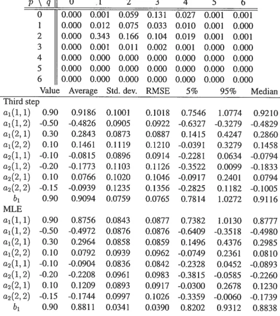
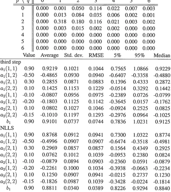
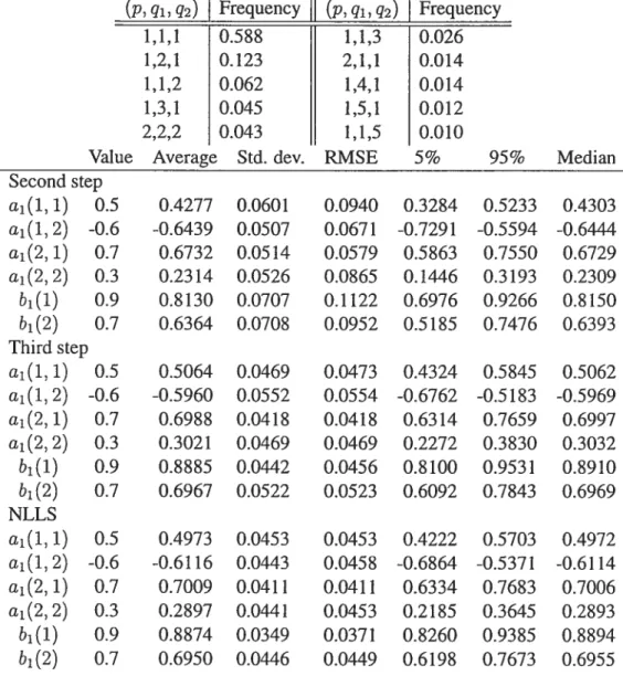
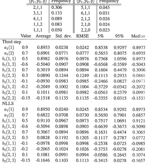
6. Monte Carlo Simulations 33

6.1. Str0ngVARMA 33

6.2. Weak VARMA 35

7. Application to macroeconomics time series 39

8. Conclusion 42

Chapter 2: Regime switching for dynamic correlations

76

1. Introduction 76

2. Ihe RSDC model 7$

2.1. Regime switching for the correlations 79

2.2. A parsimonious model $1

2.3. Univariate volatllity models 82

2.4. Review of multivariate GARCH models 84

3. Estimation $6

3.1. One-step estimation 87

3.2. Two-step estimation 90

4. Multi-step ahead condïtîonal expectations 94

5. Application to exchange rate data 98

5.1. RSDC mode! with two regimes 99

5.2. RSDC model with three regimes 101

5.3. DCC 102

5.4. Series associated to the Markov chain 104

6. Conclusion 105

7. Appendix: Proofs 107

Chapter 3: Short run and long run causality in time series:

inference

130

1. Introduction 130

2. Multiple horizon autoregressions 132

4. Causalîty tests based on stationary (p, h)-autoregressîons 141 5. Causality tests based on nonstationary (p, h)-autoregressions 145

6. Empirical il]ustration 14$

7. Conclusion 156

Chapter 4: Backtesting Value-at-Risk: a duration-based ap

proach

160

1. Motivation 160

2. Extant Procedures for Backtesting Value-at-Risk 162

3. Duration-Based Tests of Independence 164

4. Test Implementation 167

4.1. Implementing the Markov Tests 167

4.2. Implementing the Weibull and EACD Tests 169

4.3. Finite Sample Inference 170

5. BacktestingVaRs from Historical Simulation 171

6. Backtesting Tau Density Forecasts 177

7. Conclusions and Directions for Future Work 180

List

of Tables

1 _{Estimation ofa strong final MA equation form VARMA(1,1) 57}

2 _{Estimation ofa strong final MA equation form VARMA(2,1)}

5$

3 _{Estimation of a strong diagonal MA equation form VARMA(1,1). 59}

4 _{Estimation of a strong diagonal MA equation form VARMA(2,1).}

60

5 _{Estimation of a strong final AR equation form VARMA( 1,1) 61}

6 _{Estimation of a strong final AR equation form VARMA(1,2) 62}

7 _{Estimation of a strong diagonal AR equation form VARMA(1,1)}

. 63

$ _{Estimation of a strong diagonal AR equation form VARMA( 1,2)}

. 64

9 _{Estimation of a weak final MA equation form VARMA(1,1) 65}

10 _{Estimation of a weak final MA equation form VARMA(2, 1)}

66

11 _{Estimation of a weak diagonal MA equation form VARMA( 1,1)}

. 67

12 _{Estimation of a weak diagonal MA equation form VARMA(2,1)}

. 62

13 _{Estimation of a weak diagonal AR equation form VARMA(1,1)}

. 69

14 _{Estimation of a weak diagonal AR equation form VARMA(1,2)}

. 70

15 _{Estimation of a weak final AR equation form VARMA( 1,1) 71}

16 _{Unrestricted model with two regimes 113}

17 _{Unrestricted model with two regimes and GARCH 114}

1$ Restricted model with two regimes ₁₁₅

19 _{Restricted model with two regimes and GARCH 116}

20 _{Unrestricted model with three regimes}

119 21 _{Unrestricted model with three regimes and GARCH}

. 120

22 _{Restricted model with three regimes 121}

23 _{Restricted model with three regimes and GARCH 122}

24 DCC-GARCH(1,1) ₁₂₅

25 DCC-ARMACH(1,1) ₁₂₆

26 Likelihood comparison ₁₂₈

27 _{Rejection frequencies using the asymptotic distribution and the simu}

28 Causality tests and simulated p-values for series in first differences (of

logarithm) for the horizons 1 to 12 152

29 Causality tests and simulated p-values for series in first differences (of

logarithm) for the horizons 13 to 24 153

30 Summary of causality relations at various horizons for series in first

difference 154

31 Causality tests and simulated p-values for extended autoregressions at

the horizons 1 to 12 157

32 Causality tests and simulated p-values for extended autoregressions at

the horizons 13 to 24 158

33 Summary of causality relations at various horizons for series in first

difference with extended autoregressions 159

34 Power of independence tests (HS with 500 returns) 187 35 Sample selection frequency (HS with 500 retums) 186 36 Effective power of independence tests (HS with 500 retums) 189 37 Power of independence tests (HS with 250 retums) 190 3$ Sample selection frequency (HS with 250 retums) 191 39 Effective power of independence test (HS with 250 retums) 192

List of Figures

1 Macroeconomic series 72

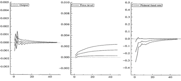
2 IRE for VAR model 73

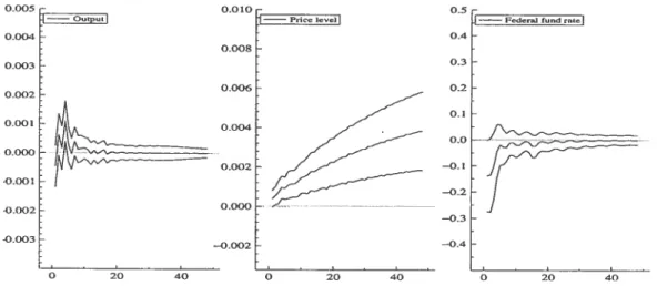
3 IRE for VARMA model in final MA equation foi-m 73 4 IRE for VARMA model in diagonal MA equation foi-m 74 5 IRE for VARMA model in final AR equation form 74 6 JRF for VARMA model in diagonal AR equation form 75 7 ACF of the cross-product of the standardized resïduals 109 $ ACF of the cross-product of the standardized residu ais (regime switch

ing) 110

9 ACF of the cross-product of the standardized residuals (DCC-GARCH) 111

10 Exchange rate series 112

11 Smoothed probabilities for the models with two regimes 117 12 Smoothed coi-relations for the models with two regimes 118 13 Smoothed probabilities for the models with three regimes 123 14 Smoothed conelations for the models with three regimes 124

15 Correlations for the DCC-ARMACH(1,1) 127

16 Smoothed probabilities and standard deviations 128 17 Conditionai variance from a GARCH( 1,1) for the return on the Dow

Jones index 129

18 Power of the test at the 5% level for given horizons . . 151

19 Value-at-Risk exceedences 182

20 Simulated returns with VaR from Historical Simulation 183 21 Simulated retums with exeedences of 1% VaR from Historical Simulation 184 22 Data-based and Weibull-based hazard functions 185 23 Histograms of duration between VaR violations 186

xi

Remerciements

J’ai de nombreuses personnes et institutions à remercier. Tout d’abord mes direc teurs de recherche, Jean-Marie Dufour et Nour Meddahi. Je m’estime chanceux d’avoir côtoyé des scientifiques et des personnes de leur calibre. J’ai très apprécié leur support moral sans lequel j’aurais sûrement abandonné en cours de route.

Je voudrais également remercier mes autres co-auteurs pour les essais de cette thèse, Peter Christoffersen et Éric Renault’. Tous deux m’ont également beaucoup appris et je suis heureux de m’être fait deux amis par le coup même.

Je voudrais également remercier les différents organismes qui m’ont accordé bourses et financements sans lesquels je n’aurais pu écrire cette thèse conseil de re cherches en sciences humaines du Canada (CRSH), Fonds québécois de la recherche sur la nature et les technologies, centre inteniniversitaire de recherche en économie quantitative (CTREQ), le centre intemniversitaire de recherche en analyse des organi sations (CIRANO). Je voudrais remercier North Carolina State University pour leur support lors de la rédaction finale de cette thèse.

Je veux remercier mon épouse Paule de m’avoir non seulement enduré, mais en couragé dans les périodes les plus exigeantes de mes études.

C

1Le premier essai a été écrit en collaboration avec Jean-Marie Dufour, le troisième avec Jean-Marie Dufour et Éric Renault, et le quatrième avec Peter Christoffersen.

C

Un des problèmes intrinsèques de l’étude des séries chronologiques multivariées est la malédiction de la dimension. Bien souvent, la complexité et le nombre de pa ramètres des modèles que l’on tente d’utiliser augmentent avec le nombre de séries chronologiques, ce qui rend l’analyse de telles séries très difficile, voire impossible. La ligne directrice de cette thèse est l’étude de méthodes permettant de contourner cette malédiction de la dimension, pour les séries tant macroéconomiques que financières.

Pour étudier la dynamique des séries chronologiques macroéconomiques, les éco nomistes se servent la plupart du temps des modèles VAR. Le grand attrait de ces mo dèles est que leur estimation ne requièrt que des régressions linéaires, ce qui les rend très faciles d’utilisation.

En revanche, l’utilisation des modèles VAR a deux grands défauts. Le premier est le manque de parcimonie. Tout comme il est admis que les modèles ARMA sont plus parcimonieux que les modèles AR pour les séries univariées, les modèles VARMA ont le potentiel d’être plus parcimonieux que les modèles VAR, surtout lorsqu’on remarque que des modèles VAR avec des ordres très élevés sont nécessaires pour de nombreuses séries macroéconomiques.

Le deuxième défaut est que la spécification d’un modèle VAR est très arbitraire puisque cette classe de modèles n’est pas robuste à l’agrégation temporelle et à la mar ginalisation. Si un vecteur suit un processus VAR, des sous-vecteurs ne suivent pas typiquement des modèles VAR (mais des processus VARMA). De la même façon, si un processus VAR est observé à une fréquence différente, alors la série obtenue ne suit pas un modèle VAR mais un processus VARMA. Par opposition, l’agrégation temporelle ou la marginalisation d’un processus VARMA demeure un processus VARMA.

Les économistes persistent tout de même à utiliser seulement les modèles VAR au lieu d’envisager les modèles VARMA, ce qu’on peut expliquer par deux raisons. La première est que la représentation VARMA identifiée privilégiée par la littérature éco nométrique, i.e. la forme échelon, est difficile à manipuler. L’utilisateur doit spécifier

s. _{les indices de Kronecker (le nombre d’indices est égal au nombre de séries), et les}

sition relativement à la diagonale. La seconde raison est que la méthode d’estimation habituellement proposée pour les modèles VARMA est le maximum de la vraisem blance. Les modèles VARMA sont plus parcimonieux que les modèles VAR mais le nombre de paramètres peut être élevé, ce qui rend très compliquée la maximisation de la vraisemblance.

Dans le premier essai de cette thèse, nous présentons une méthode pour la modéli sation des modèles VARMA qui franchit ces deux obstacles. Dans un premier temps, nous introduisons deux nouvelles représentations VARMA identifiées, lafonne équa tion diagonale MA et lafonne équation finale MA, où les opérateurs MA sont respec tivement diagonaux et scalaires. Ces représentations ont de nombreux avantages. Elles peuvent être interprétées comme de simples extensions du modèle VAR. Contrairement à la forme échelon, elles imposent une forme très simple sur la partie MA, celle qui complexifie l’utilisation des modèles VARMA. Les ordres des polynômes qui compose la partie MA ne sont pas reliés entre eux, contrairement à la forme échelon.

Dans un second temps, nous proposons une méthode d’estimation qui ne requiert que trois régressions linéaires. Cette méthode est une généralisation de celle proposée par Hannan et Rissanen (1982) pour les modèles ARMA. Les estimateurs de la troi sième régression ont les mêmes propriétés asymptotiques que ceux obtenus par maxi mum de vraisemblance sous l’hypothèse que les innovations sont gaussiennes. Avec cette méthode d’estimation, nous combinons un critère d’information qui donne des estimations convergentes des ordres des polynômes AR et MA.

Pour l’étude des séries financières, la malédiction de la dimension force les éco nomistes à utiliser des modèles aux dynamiques très simples. Les généralisations mul-tivariées directes des modèles GARCH univariés, tel que le modèle BEKK de Engle et Kroner (1995), ne peuvent être appliquées à plus de quatre ou cinq séries sans quoi la maximisation de la vraisemblance devient prohibitive [voir Ding et Engle (2001)]. Une avenue intéressante pour la spécification des modèles de volatilité multivariés est la décomposition des covariances en corrélations et écarts types. Le chercheur spécifie ensuite des modèles pour les écarts types et un modèle pour la matrice de corrélation. On se débarrasse ainsi de la malédiction de la dimension puisqu’on peut estimer le modèle deux étapes d’abord pour les écarts types puis ensuite pour la matrice de

cor-rélation en utilisant les résidus standardisés. Le premier à utiliser cette décomposition a été Bollerslev (1990), en posant l’hypothèse que les corrélations sont constantes.

L’hypothèse selon laquelle la matrice de corrélation est constante n’étant pas tou jours appuyée par les données, de nouveaux modèles ont été proposés au cours des dernières années. Les modèles Dynamic Conditionat Corretations de Engle (2002) et Multivariate GARCH de Tse et Tsui (2002) avancent plutôt une dynamique de type GARCH pour la matrice de corrélation la matrice de corrélation est aujourd’hui une fonction des matrices de corrélation passées et des produits croisés des innovations standardisées passées.

On préfère ces modèles à ceux qui ont une matrice de corrélation constante, mais une dynamique de type GARCH pour la matrice de corrélation n’est pas entièrement satisfaisante. Le fait que les produits croisés des innovations standardisées ne soit pas borné par -1 et 1 est un problème, puisque cela implique qu’aucun élément de la matrice de corrélation n’est borné par -1 et 1. Par conséquent, on doit remettre à l’échelle les matrices obtenues afin de vraiment aboutir à des matrices de corrélation, mais ces mises à l’échelle introduisent des non-linéarités qui ont pour effet d’empêcher les calculs ana lytiques d’espérance conditionnelle pour les covariances et corrélations. On s’aperçoit qu’un modèle qui ne tient pas directement compte des caractéristiques d’une matrice de corrélation n’est pas satisfaisant.

Dans le deuxième essai, nous proposons un nouveau modèle de volatilité multiva né, le modèleRegime Switching Dynamic Corretation. Nous décomposons également les covariances en corrélations et écarts types, mais la matrice de corrélations suit un modèle à changement de régime elle est constante à l’intérieur d’un régime mais dif férente entre régimes. Les transitions entre régimes sont déterminées par une chaîne de Markov. Ce modèle ne souffre pas d’une malédiction de la dimension puisqu’on peut l’estimer en deux étapes, tout comme les modèles de Bollerslev (1990), Engle (2002), Tse et Tsui (2002). Notre modèle a aussi l’avantage de permettre le calcul analytique d’espérance conditionnelle sur plusieurs horizons de la matrice de corrélation, et de la matrice de variance si un modèle approprié pour les écarts types est employé [le modèle ARMACH de Taylor (1986)]. Nous présentons également une application empirique qui montre que notre modèle peut avoir une meilleure performance inter-échantillon

que celui d’Engle (2002).

Les tests de causalité à plusieurs horizons, tel que définis dans Dufour et Re nault (199$), présentent également des problèmes associés à l’étude des séries ma croéconomiques multivariées. Même dans les modèles VAR, les hypothèses de causa lité à plusieurs horizons sont non linéaires et prennent la forme de contraintes sur des transformations multilinéaires des paramètres du modèle VAR. L’application des tests statistiques habituels, de type Wald, par exemple, pourrait générer des matrices de cova riance asymptotiquement singulières, avec comme résultat que la théorie asymptotique standard ne s’appliquerait pas à ces statistiques.

C’est pourquoi nous présentons, dans le troisième essai, des méthodes de test simples pour tester les hypothèses de non-causalité à plusieurs horizons dans les mo dèles VAR d’ordre fini qui ne requièrent que des méthodes de régression linéaire. Celles-ci méthodes sont basées sur des autorégressïons vectorielles à multiples hori zons où on peut estimer les paramètres au moyen de méthodes linéaires. En utilisant cette approche, on peut tester les restrictions de non-causalité à divers horizons en uti lisant des critères de type WaId ou fisher, une fois que l’on tient compte de la structure moyenne mobile des erreurs (qui sont orthogonales aux régresseurs).

Une des raisons d’être des modèles de volatilité multivariés tels que celui que nous présentons dans le deuxième essai est de prédire la distribution de rendements futurs d’un portefeuille. Ces prédictions sont nécessaires pour le calcul de la Valeur-à-Risque (VaR) d’un portefeuille d’actifs financiers. La VaR d’un portefeuille est tout simple ment un quantile de la distribution des rendements futurs du portefeuille. C’est une mesure du risque d’un portefeuille: plus ses rendements sont volatils, plus la variance est élevée, et plus les petits quantiles sont éloignés de la moyenne. Les institutions fi nancières sont maintenant tenues de calculer ces VaR par, notamment, les Accords de Basle.

Dans le quatrième essai, nous présentons de nouveaux tests statistiques pour évaluer si le modèle utilisé pour calculer la VaR est correctement spécifié. Si aujourd’hui la VaR pour demain et pour un niveau de couverture de 1 % est 10 000$, cela signifie que demain, la probabilité que ce portefeuille perde plus que 10 000$ est égale à I %. L’évaluation des modèles utilisés pour calculer les VaR est basée sur la comparaison

des VaR (ex-ante) et des pertes effectives (ex-post). On crée ainsi une séquence binaire

‘t on marque un 1 pour les jours où les pertes excèdent la VaR et un O pour les jours

où la VaR n’excède pas les pertes.

Si la VaR est calculée de façon optimale, il devrait être impossible de prévoir à quel moment elle sera violée (quand les pertes vont excéder la VaR), ce qui implique que la séquence‘t devrait être indépendante. Si on calcule une VaRavec un niveau de

couverture de p%, alors on devrait excéder la VaRp % des jours. Donc, ce qui nous intéresse, c’est de vérifier si la séquence I est i.i.d. Bernoulli(p). Des tests basés sur l’hypothèse alternative d’une chaîne de Markov pour décrire la séquence I ont été avancés par Christoffersen (199$).

Dans cet essai, nous proposons des nouveaux tests statistiques qui sont basés sur la durée en nombre de jours entre les violations de la VaR. Si le modèle utilisé pour calculer la VaR est optimale, alors ces durées devraient être i.i.d. exponentielles de moyenne l/p. S’il est impossible de prévoir quand la VaR sera violée, il ne peut y avoir d’effet de mémoire et si la VaR est excédée p % du temps, on devra attendre 1/pjours en moyenne entre les violations. Pour tester cette hypothèse, nous proposons deux alternatives qui englobent le cas i.i.d. exponentiel la distribution Weibull et le modèle EACD de Engle et Russe! (199$).

À

l’aide de simulations Monte Carlo, nous montrons que pour des situations réalistes, ces tests ont plus de puissance que ceux proposés précédemment.

VARMA models with a

macroeconomic application

1.

Introduction

In time series analysis and econometrics, VARMA models are scarcely used to repre sent multivariate time series. VAR models are much more widely employed because they areeasier to implement: the latter models can be estimated by least squares meth ods, while VARMA models typically require nonlinear methods (such as maximum likelihood).

VAR models, however, have important drawbacks. First, they are typically much less parsimonious than VARMA models. Second, the family of VAR models is flot closed under marginalization and temporal aggregation. If a vector satisfies a VAR model, subvectors do flot typically satisfy VAR models (but VARMA models). Simi larly, if the variables of a VAR process are observed at a different frequency, the resuit ing process is flot a VAR process. In contrast, the class of (weak) VARMA models is closed under such operations. We say that a VARMA model is strong if the innovations are independent, and it is weak if they are merely uncorrelated.

It follows that VARMA models appear to be preferable from a theoretical view point, but their adoption is complicated by identification issues and estimation difficul ties. The direct multivariate generalization of ARMA models does flot give an identified representation. It follows that a one has to decide on a set of constraints to impose so as to gain identification. Standard estimation methods for VARMA models (maximum likeÏihood, nonlinear least squares) require nonlinear optimization which may not be feasible as soon as the model ïnvolves a few time series, because the number of param eters can increase quickly.

In this paper, we consider the problem of estimating VARMA models by relatively simple methods which only require linear regressions. For that purpose, we consider

a generalization by Hannan and Kavalieris (19$4a) of the regression-based estimation method proposed by Hannan and Rissanen (1922) for unïvariate ARMA models. Their method is performed in three steps. In a first step a long autoregression is fitted to the data. In the second step, the lagged innovations in the ARMA model are replaced by the corresponding residuals from the long autoregression and a regression is per formed. In a third step, the data from the second step arefiltered so as to give estimates that have the same asymptotic covariance matrix than one would get with the maximum likelihood [claimed in Hannan and Rissanen (1982), proven in Zhao-Guo (1985)]. Ex tension of this innovation-substitution method to VARMA models was also proposed by Koreïsha and Pukkila (1989), but these authors did not provide a detailed asymptotic theory for their proposed extension.

Here, we first provide such a theory by showing that the linear regression-based esti mators are consistent under weak hypotheses on the innovations and how filtering in the third step gives estimators that have the same asymptotic distribution as their nonlinear counterparts (maximum likelihood if the innovations are independent and identically distributed (i.i.d.), or nonlinear least squares if they are merely uncorrelated). In the non i.i.d. case, we consider strong mixing conditions [Doukhan (1995), Bosq (1998)], rather than the usual martingale difference sequence (m.d.s.) assumption. By using weaker assumptions for the process of the innovations we broaden the class of models to which our method can be applied.’

Second, in order to avoid identification problems and to further ease the use of VARMA models, we introduce three new identified VARMA representatÏons, the diag onatMA equationfonn, thefinalMA equationform and the diagonalAR equationfonn. Under the diagonal MA equation form (diagonal AR equation form) representation, the MA (AR) operator is diagonal and each lag operator may have a different order qj (p). Under the final MA equation form representation the MA operator is scalar, i.e. the the operators are equal across equations. The diagonal and final MA equation form repre sentations can be interpreted as simple extensions of the VAR model, which should be appealing to practitioners who prefer to employ VAR models due to their ease of use.

‘For univariate ARMA models Francq and Zakoïan (1998) presents numerous cases where the rep resentation is only weak.

The identified VARMA representation that is the most widely employed in the litera ture is the echelon fonn. Specification of VARMA models in echelon form does flot amount to specifying the order p and q as with ARMA models. Under this representa tion, VARMA models are specified by as many parameters, called Kronecker indices, as the number of time series studied. These indices determine the order of the elements of the AR and MA operators in a non trivial way. The complicated nature of the ech elon form representation might be a reason why practitioners are not using VARMA models, so the introduction of a simpler identified representation is interesting. The proposed representations may be less parsimonious than the echelon form but since our estimation method only involve regressions we can afford it.

Thirdly, we suggest a modified information criterion to choose the orders of VARMA models under these representations. This criterion is to be minimized in the second step of the estimation method over the orders of the AR and MA operators and gives consistent estimates of these orders. Our criterion is a generalization of the infor mation criterion proposed by Hannan and Rissanen (1982), which was corrected later on in Hannan and Rissanen (1983, 1984b), for choosing the orders p and q in ARMA models. The idea of generalizing this information criterion is mentioned in Koreisha and Pukkila (1989) but a specific generalization and theoretical properties are flot pre sented.

Fourth, the method is applied to U.S. macroeconomic data previously studied by Bemanke and Mihov (1998) and McMillin (2001). To illustrate the impact of using VARMA models instead of VAR models to study multivariate time series we compare the impulse-response functions generated by each model. We show that we can ob tain much more precise estimates of the impulse-response function by using VARMA models instead of VAR models.

The rest of the paper is organized as follows. Our framework and notation are in troduced in section 2. The new identified representations are presented in section 3. In section 4, we present the estimation method. In section 5, we describe the infor mation criterion used for choosing the orders of VARMA models under the represen tation proposed in our work. Section 6 contains resuits of Monte Carlo simulations which illustrate the properties of our method. Section 7 presents the macroeconomic

application where we compare the impulse-response functïons from a VAR model and VARMA models. Section _{8 contains a few concluding remarks. Finally, proofs are in} the appendix.

2.

Framework

Consider the following K-variate zero mean VARMA(p,q) model in standard represen tation:

Yt = + U

- (2.1)

where U is a sequence of unconeÏated random variables defined on some probability space ($2, A, P). The vectors _{and U contain the K univariate time series: =} [yt(1), yt(2), .. . ,y(K)]’ and U = [u(1), ut(2), . . . zt(K)]’. We can also write the

previous equation with lag operators:

A(L)Y = B(L)U (2.2)

where

A(L) = ‘K — A1L — •.• — (2.3)

3(L) = IKB1L ““3qV. _(2.4)

Let H be the Hilbert space generated by (Y, s < _{t). The process (Ui) can be}

interpreted as the linear innovation of Y:

Ut=Y—EL[}’jHtJ. _(2.5)

Also assume that _{is a strictly stationary and ergodic sequence and that the process} {U} has common variance (Var[UtJ =

)

and finite fourth moment (E[Iu(i)I426} _< œ for some 5 > O). We make the zero mean-mean hypothesis only to simplify the

notation.

Assuming that the process

_{}

is stable,

det [A(z)] O for

IzI

< 1, (2.6)

and invertible,

det[3(z)J Oforlz

<1, (2.7)

it, can 5e represented as an infinite VAR

H(L)Y = U, where H(L) = B(L)’A(L)=IK—ZHiL, or an infinite VMA = where 1(L) = A(L)’B(L)=IK—ZPjL. i=1

The matrices H and !P could be zero past a finite order if det[B(L)] or det[A(L)1 respectively is a non-zero constant. We will denote by a(L) the polynomial in row i and column

_j

of A(L), and the row i or coïumn

j

of A(L) by

A, (L) ₌ [ail(L), .. . ,aK(L)], (2.)

o

The diagoperator creates a diagonal matrix,

diag[a(L)j = diag[aii(L),. . ._, aii(L) O = _{, (2.10)} O aKK(L) where a(L) = — — — (2.11)

The function deg[a(L)] returns the degree of the polynomial a(L) and the function dirn(7) gïves the dimension of the vector .

We need to impose a minimum of structure on the process {U} because saying that it is uncorrelated is flot enough to get any significant results. The typical hypothesis that is imposed in the time series literature is that the U’s are either independent and identically distributed (i.i.d.) or a martingale difference sequence (m.d.s.). In this work we do not impose such strong assumptions because we want to broaden the class of models to which it can be applied. We only assume that it satisfies a strong mixing condition [Doukhan (1995), Bosq (1998)]. Let {U} be a strictly stationary process, then its c-mixing coefficient of order h is defined as

c(h) = sup

I

Pr(B

n

C) — Pr(B) Pr(C)I , h 1. (2.12)

5ErfUs,s<t) CE_“fU5,s t+h)

The strong mixing condition that we impose is

<œ for some >0. (2.13)

h= 1

3.

Diagonal VARMA representations

It is important to note that we cannot work with the standard representation (2.1) be cause it is flot identified. To help us gain intuition on the identification of VARMA models we can consider a more general representation where A0 and B0 arenot iden tity matrices:

A0 = A1Y1 + + ApYp + B0Û

— B1Û1 + +BqUtq. (3.1)

By this specification, we mean the well-defined process

= (A0—A1L— ..._ALP)_l(B0+B1L±...+BL)Û(t).

But we can see that such process has a standard representation if A0 and B0 are non-singular. To see this we left-multiply (3.1) by A0 and define Ut = A0’BoUt:

= A0’A1Y1 + + A0’A + U(t) —

A0’B1Bo’A0U1 — . — Ao’BqBo’AoUt_q.

Redefining the matrices we get a representation of the type (2.1). With this example we see that as long as A0 and B0 are non-singular we can transform a non-standard VARMA into a standard one.

We say that two VARMA representations are equivalent if A(L)’B(L) resuits in the same operator !P(L). Thus, to insure uniqueness of a VARMA representation we must impose restrictions on the AR and MA operators such that for a given !P(L) there is one and only one set of operators A(L) and B(L) that can generate this infinite MA representation.

A first restriction that we impose is a multivariate equivalent of the coprime prop erty in the univariate case. We don’t want elements of A(L) and B(L) to “cancel out” when we take A(L)’B(L). We cail this the Ïeft-coprirne property [see Han nan (1969), Lûtkepohl (1993a)]. It may be defined by calling the matrix operator P[A(L), 3(L)] = A(L)1B(L) Ieft-coprime if the existence of operators D(L), À(L),

and (L) satisfying

D(L)[À(L), (L)] = !P[A(L), B(L)1 (3.2)

implies that D(L) is unimodular, that is det D(L) is a nonzero constant. To obtain uniqueness of left-coprime operators we have to impose restrictions ensuring that the only feasible unimodular operator D(L) in (3.2) is D(L) = ‘K There exist more

than one representation which guarantee the uniqueness of the left-coprime operators. The predominant representation in the literature is the echeton form [see Deistier and Hannan (1981), Hannan and Kavalieris (1984b), Ltitkepohl (1993a), Ltitkepohl and Poskitt (1996a)].

Definition 3.1 (Echelon form) Tue VARMA representation in (2.1) is said to be in echeton fonn tf Hie AR and MA operators A(L) = [a5(L)],=i _K and 3(L)

[bjj

(L)1,=i

K satisfy the foitowing conditions: ail operators (L) and (L) in

the i-th row ofA(L) and 3(L) have Hie same degree p and have thefonn

a(L) 1_ajj,mLm, _fori=l,..,K

m=1

a(L) = — aiLm, forj j

m=pj —p,+ 1

(L) = bi,Ltm for i,

j

= 1, .. . ,K, with B A0.

m=O

Furthe,; in Hie VAR operator ajj (L),

f

min(pi + i,p) fori >

_j

Pij=

I min(p,p) fori<j

i.e., Pij specifies the nurnberoffree coefficients in the operatora(L)forj i. The row orders (pi, .. . ,pK) are the Kronecker indices and their sum pi is the McMittan

degree. For the VARMA orders we have in generai p = q = mar(py,. . . ,pjç).

We see that dealing with VARMA models in echelon form is flot as easy as dealing with univariate ARMA models where everything is specified by choosing the value of

p and q. The number of Kronecker indices is bigger than two (if K is bigger than two) and when choosingPij we have to consider if we are above or below the diagonal. Having a summation subscript in the operator a, m = p — Pij + 1, different across

rows and columns also complicates the use of this representation. The task is far from being impossible but it is more complicated than for ARMA models. Specification of VARMA models in echelon form is discussed in Hannan and Kavalieris (1984b), Ltitkepohl and Claessen (1997), Poskitt (1992), Nsiri and Roy (1992), Nsiri and Roy (1996), Lûtkepohl and Poskitt (1996b), Bartel and Ltitkepohl (199$). This might be a reason why practitioners are reluctant to employ VARMA models. Who could blame them for sticking with VAR models when they probably need to refer to a textbook to simply write down an identified VARMA representation?

In this work, to ease the use of VARMA models we present new VARMA repre sentations which can be seen as a simple extensions of the VAR mode!. To introduce them, we first review another identified representation, the final equationform, which will refer to as the final AR equationfonn, under which the AR operator is sca!ar {see Zel!ner and Pa!m (1974), Hannan (1976), Wa!!is (1977), Ltitkepohl (1993a)].

Definition 3.2 (Final AR equation form) The VARMA representation (2.1) is said to be infinatAR equationfonn if 11(L) a(L)IK, where a(L) 1— a1L — ... — aL?

is a scatar polynomial with a O.

To see how we can obtain a VARMA mode! with a final AR equation form repre sentation, we can proceed as follows. By standard linear algebra, we have

A*(L)A(L) = A(L)A(L)* _{det [11(L)]}

‘K

where A*(L) is the adjoint matrix of 11(L). On muhiplying both sides of (2.2) by A*(L), we get:

det [11(L)] Y = A(L)*B(L)Ut.

This representation may flot be attractive for severa! reasons. First, it is quite far from usual VAR models by exciuding !agged values of other variables in each equation

[e.g., the ARpart_{of the first equation ïnclude lagged values of yt(1) but no lagged val}

ues of yt(2),. . - ,yt(K)]. Further, the AR coefficients are the same in ail the equations, which wiil require a polynomial of higlier order (p K). Second, the interaction between the different variables are _{modeled through the MA part of the model, which may have}

to be quite complex.

We can obtain our new representations with analogous manipulations. Upon muiti plying both sïdes of (2.2) by B*(L), we get:

B(L)*A(L) _{= det [3(L)] Ut}

(3.3) where B(L)* is the adjoint mati-ix of 3(L). We refer to VARMA models in (3.3) as being in final MA equationfonn.

Definition 3.3 (Final MA equatïon_{form) The VARMA representation (2.1) is said to}

hein final MA equationfonn if 3(L) = b(L)IK, where b(L) = 1 — b1L — ... — bqL1

is a scalar operatorWith bq O.

The same criticism regarding the parsimony of the final equation fonu would apply but it is possible to get a more parsimonious rcpresentation by looking at common structures across equations. Suppose there are common roots across rows for some coiumns of 3(L), so that starting from (2.1) we can write

= È(L)D(L)U

= det [B(L)] D(L)U _(3.4)

where D(L) = diag[di(L), . . . ,dK(L)] and d(L) is a polynomial common to

Vi = 1,. . . ,K. We see that aliowing non-equal diagonal polynomials in the moving

average as in equation (3.4) may give a more parsimonious representation than in (3.3). We will cail the representation (3.4) diagonal MA equationform representation.

Q

Definition 3.4 (Diagonal MA equatïon form) The VARMA representation (2.1) is said to be in diagonal MA equationfonn if 3(L) diag[b(L)] = Ii — B1L — ... — BqL” where b(L) 1 b,iL — ... — bji,qjL, bijq O, and q ₌ maxl<j<K(qj).

This representation is interesting because contrary to the echelon form it is easy to specify. We don’t have to deal with mies for the orders of the off-diagonal elements in the AR and MA operators. The fact that it can be seen as a simple extension ofthe VAR model is appealing. Practitioners are comfortable usïng VAR models, so simply adding lags of u(t) to equation j is a natural extension of the VAR model which could give a more parsimonious representation. It also has the advantage of putting the simple structure on the MA part, the part_{which complicates the estimation, instead of on the}

AR part as in the final AR equation form. Notice that in VARMA models, it is flot necessary to include lags of ail the innovations u1(t), ,ujç(t) in every equations. This couid entice practitioners to consider VARMA models if it is combined with a simple regression-based estimation method. For this representation to be useful, it needs to be identified. This is demonstrated in Theorem 3.11 below under the following assumptions and using Lemma 3.8 below

Assumption 3.5 The matrices A(z) and 3(z) have thefoÏlowingfonn:

A(z) = IK—AlZ—»—AZ

3(z) = I_B1z__3qz

Assumption 3.6 B(z) is diagonal:

3(z) diag [b(z)j

with b(z) = 1 — biz — bjjqjzi, biiqi O.

Assumption 3.7 For each j = 1, .. . K, there are no roots common to A.(z) and b(z), i.e. there is no value z such that A.(z*) = O andbjj(z*) = O.

Lemma 3.8 Let [A(z), 3(z)] and [À(z). B(z)] be twopairs of polynomial matrices which satisfy the asswnptions 3.5 to 3.7. If R0 is a positive constant such that

det[A(z)]

O,det[3(z)]O det {À(z)]

O, det

[B(z)] O

forO < z <R0, and

A(z)’B(z) = À(z)’(z)

forO <

_IzI

<R0, then

11(z) À(z) andB(z) = B(z),Vz

Remark 3.9 In Lemma 3.8, the conditïon

A(z)’B(z) = À(z)’(z)

could be replaced by

B(z)’A(z) = B(z)’À(z)

since by assumption the inverse of B(z) and B(z) exist.

Remark 3.10 The assumptions 3.5 to 3.7 and conditions in Lemma 3.8 allow

det[A(z)] and det[B(z)} to have foots Ofl or inside the unit circle z = 1.

PROOF 0F LEMMA 3.8 Clearly, 11(0) = 3(0) _{= ‘K} and det[A(0)] = det[B(0)] = 1 _{0. The polynomials det[A(z)] and det[B(z)] are different from zero in a neigh} borhood of zero. In particular, we can choose R0 > O such that det[A(z)] O and

det[B(z)] O for O < zj < _{R0. It follows that the matrices A(z) and 3(z) are}

invertible for O <

Izl

< R0.

Let

Co={zeCI0<zI<Ro}

and

1$ for z E G0. Since = det[A(z)]’ = det[B(z)j’

where A*(z) and B*(z) are matrices of polynomials, it follows that, for z E Go, each element of A(z)’ and B(z)’ is a rational function whose denominator is different from zero. Thus, forz é G0, A(z)1 and B(z)1 are matrices of analytic functions. It follows that the function

!P(z) = A(z)’B(z)

is analytic in the circle O z <R0. Hence, it lias a unique representation of the form

(z)=kz’, zéG0.

By assumption,

(z) = A(z)1B(z) = À(z)’B(z)

for z E G0. Hence, for z E G0,

À(z)A(z)’B(z) = B(z)

À(z)A(z)’ = B(z)B(z)’ A(z) (3.5)

where L\(z) is a diagonal matrix because B(z) andB(z) are both diagonal,

A(z) = diag [6(z)],

where

G

= b(z)

19

From (3.6), it follows that each 6(z) is rational with no pole in C0 such that 6(O) = 1,

so it can be written in the form

6(z) =

where e(z) and f(z) have no common roots, f(z) O for z E Co and 6(O) e(O) = 1.

From (3.5), ït follows that for j = 1, . . . ,K,

=

= 6(z)a(z),

j

= 1,...,K,

for z E C0.

We first show that(z) must be a polynomial. If f(z) 1, then its order cannot be greater than the order qi deg[b(z)J for otherwisei(z) would flot be a polynomial. Similarly, iff(z) 1 and is a polynomial of order less or equal to qj, then all its roots must be roots of b(z) and a(z), for otherwise b(z) or âj(z) would be a rational function. If qj > 1, these foots are then common to b(z) and a(z),

j

= 1, . .. ,K,

which is in contradiction with Assumption 3.7. Thus the degree of f(z) must be zero, and 5(z) is a polynomial.

If 6(z) is a polynomial of degree greater than zero, this would entai! that

bjj

(z) and (z) have roots in common, in contradiction with Assumption 3.7. Thus (z) must be a constant. Further, S(O) = 1 so that for j = 1,. . . , K,

bjj(z),

= a(z),

j

= 1. . . ,K,

and

O

B(z) =

It should be noted that Assumption 3.7 is weaker than the hypothesis that det[A(L)] and det[B(L)J have no common roots, which would be a generalization of the usual identification condition for ARMA models.

Theorem 3.11 IDENTIFICATION 0F DIAGONAL MA EQUATION FORM REPRESEN

TATION. UnderAssumptions 3.5, 3.6, 3.7, and the assumption that the VARMA process is invertible, VARMA models in diagonal MA equationforni are identtfied.

PR00F 0F THE0REM 3.11 Under the assumption that the VARMA process isinvert ible, we can write

= U

Now suppose by contradiction that there exist operators À(L) and B(L), with B(L) diagonal and invertible, andÀ(L) A(L) or (L) L B(L), such that

B(L)-1À(L) = B(L)’A(L)

If the above equality hold, thenitmust also be the case that

(z)’À(z) = B(z)’A(z), Vz E C0

where C0 = {z E C

I

O < zI <R0} and R0 > 0. By Lemma 3.8,itfollows that

À(z) = A(z)

B(z) = B(z) Vz.

Hence, the representation is unique. D

()

Similarly, we can demonstrate that the final MA equation form representation is identified under the following assumption.

Assumption 3.12 There are no roots common to A(z) and b(z), i.e. there is no value

z such that A(z*) = O and b(z*) = O.

Theorem 3.13 IDENTIFICATION 0F FINAL MA EQUATION FORM REPRESENTA

TION. UnderAssumption 3.12, _{VARMA modets in final MA equationform are identi} fied.

PR00F 0F THE0REM 3.13 The proof can be easily adapted from the proof of Theo

rem3.11 once wereplace Assumption 3.7 by Assumption 3.12.

LI

Looking at equation (3.3), we see that it is aiways possible to obtain a diagonal MA equation form representation starting from any VARMA representation. One case where we would obtain a diagonal and not final MA representation is when there are common factors across rows of columns of3(L) as in (3.4).

One strong appeal of the diagonal and final MA equation form representations is that it is really easy to get the equivalent (in term of autocovariances) invertible MA representation of a non-invertible representation. With ARMA models, we simply have

to invert the foots of the MA polynomial which are inside the unit cïrcle and adjust the standard deviation of the innovations (divide it by the square of these roots), see

Hamilton (1994, Section 3.7). The same procedure could be applied to VARMA models

in diagonal or final MA equation form.

for VARMA representations where no particular simple structure is imposed on the

MA part, at the moment we are not aware of an algorithm to go from the non-invertible to the invertible representation tough theoretically this invertible representation exist and is unique as long as det[B(z)] O for z 1 [see Hannan and Deistier (1988, chapter 1, section 3)]. So it might be troublesome to use a nonlinear optimization with these VARMA representations since we don’t know how to go from the non-invertible

to the invertible representation.

We can also consider the following natural generaÏization of the final AR equation form, where we simply replace the scalar AR operator by a diagonal operator.

said to be in diagonal AR equation form if A(L) = diag[a(L)] = ‘K — A1L —

— API? where a(L) = 1 — a,1L — ... — andp = maxl<j<K(pj).

Assumption 3.15 For each j = 1, .. . ,K, there are no roots common to a(z) and

B.(z), i.e. there is no value z such that ajj(z*) O and B.(z*) = O.

Theorem 3.16 IDENTIFICATION 0F DIAGONAL AR EQUATION FORM REPRESEN

TATION. Under Assumption 3.15, VARMA models in diagonal AR equation form are identified.

From Theorem 3.11 we cari see that one way to ensure identification is to impose constraints on the MA operator. This is an alternative approach to the ones developed for example in Hannan (1971, 1976) where the identification is obtained by restricting the autoregressive part to be lower triangular with deg[a(L)] deg[a(L)] for

_j

> j,

or in the final AR equation form where A(L) is scalar. It may be more interesting

to impose constraints on the moving average part instead because it is this part which causes problems in the estimation of VARMA models. Other identified representations which do flot have a simple MA operator include the reversed echelon canonical form [see Poskitt (1992)] where we permute the rows of the VARMA model in echelon form so that the Kronecker indices are ordered from smallest to largest, and the scalar component model [see Tiao and Tsay (1989)] where we study contemporaneous linear transformations of the vector process. A general treatment of algebraic and topological structure underlying VARMA models is given in Hannan and Kavalieris (1984b).

4.

Estimation Method

We next intro duce elements of notation for the parameters of our model. First, irrespec tive of the VARMA representation employed we spiit the whole vector of parameters 7 in two parts 7 (the parameters for the AR part) and72 (MA part):

For a VARMA model in diagonal MA equation form, _‘y and72 are

7i = [ai.,i,. . .,a1.,,. . .,aK.,1,.. . , (4.1)

72 = [b11,1,. . -, bii,q1,.. . , - , (4.2)

while for a VARMA model in final MA equation form, ₇₂

72 = [b1, . . . ,bq}. (4.3)

For VARMA models in diagonal AR equation form, we simply invert ‘y and 72:

= [an;,-. . ,an,1, . . - ,KK,i, - ,aKK,Pl (4.4)

72 = [b1.,, bi.,q, - ,bK.,l, - - ,bK.,ql , (4.5)

while for a VARMA model in final AR equation form,‘y is

(4.6)

The estimation method is in three steps.

Step 1. Estimate a VAR(nT) to approxÏmate the VARMA(p,q) and recuperate the residuals that we will cail

_Û:

= — ft1(nw (4.7)

withT> 2 x K x riT.

Step 2. With the residuals from step 1, compute an estimate of the variance matrix of U,

ÛÛ/T

and estimate by GLS the following multivarïate regres sion:

to get estimates Â(L) and.(L) of A(L) andB(L). The regression is

=

[>_-‘]

with t = T +max(p, q) + 1. If we define the following vectors

Y_1 = [y_y(i), .. . ,yt_i(K),.. . ,yt-(l),.

. .

,y_(K)]

Û_1

= [û_1(1),. . . ,ût_1(K), ,t_q(1), ,

t_q(K)]

y_i(k) = [yt_l(k),...,yt_pk(k)Ï

û_1(k) [û_1(k), . . ,Ût_q(k)]

then the matrix Z_i for the various representations is

Yt—l O O •.. Yt_i Yt_l O FMA Lit_1 — O •.. Y_i Yt-i(l) ‘3’DAR Lit_l — O Yt—i(1) Ût_l 5’FAR Lit_l — yt_i(K) O (4.8) DMA Lit_l Ût_i(1) O O •.• û_1(K) û_1(1) û_1(K) Ui_1 “. O O O Ui_1 O

O

Û_1

O yt_i(K)

o

where DMA, FMA, DAR and FARrespectively stands forDiagonal MA, Final MA, Diagonal AR and Final AR equation form.

Step 3. Using the second step estimates, we first form new residuals

=

- +

initiating with U = O, t max(p,q), and we define

=

=

initiating with X W = O for t max(p,q). We also compute a new estimate of,

t=max(p,q)+1 ÙÙ/T. Then we regress by GLS

Ùt

+X — W on with

=

where is just like

2

from step 2 except that it is computed with

Ù

instead of

Û

to obtain regression coefficients that we cail

Â

and

Ê:

—1

. (4.9) t=max(p,q)+1 t=max(p,q)+1

The properties of the estimation method are summarized in the following three theorems. Theorem 4.1 is a generalization of resuits from Lewis and Reinsel (1985) where convergence is demonstrated for i.i.d. innovations. We denote the Euclidean norm by

113112

= tr(B’B).

Theorem 4.1 VARMA FIRSI STEP ESTIMATES. Under the above hypothesis on Hie process {}‘} and fnT grows at a rate faster than log T withnT2/T —÷ O then for the

first stage estirnates _IlHt(n) —

Hill

O.

Theorem 4.2 VARMA SECOND STEP ESTIMATES. Under Hie above hypothesison

the process

_{}

and ifriT grows at a rate faster than log T with nT2/T —* O then the

Theirasyinptoticdistribution is given by

(—7) (4.10)

with

ï

= E

[{z1E-’u}

J

E

[z_1z-’z_1]

and Z_1 is equat to the matrix _{2_i} where

Û

is replaced by U.

Also, if m/T —* O with mT —* oc then the matrix I and J can be consistently

estimated in probability respectivety by

m1 T ÏT = w(j,mT) (4.11) tt+IjI JT = (4.12) with w(j,rnT) = 1 — j/(mT + 1).

Theorem 4.3 VARMA THIRD STEP ESTIMATES. Under the above hypothesis on the process {Y} and ifnTgrows at a rate faster titan logT with nT2/T —* O then the

third stage estimates converge in quadratic mean to tizeir true value. Their asymptotic distribution is giveiz by

(-)

(O,J’ÎJ1) (4.13)

with

Ï

= E

[{v1E-’u}

j=-œ

J

=

Atso, tf m/T — O with mT — œ tïteïz the matrix

Î

and

J

can be consistentÏy

estirnated in pro bability respectivety by

mT T

Î1

=

>

w(j,m)

{1’û}

(4.14)

j=—mr t=t’+j

j1 = (4.15)

t=max(p,q)+1

with t’ max(p, q) + 1 and

U

are thefiïtered residuats computed with

_5’.

Notice the simplicity of this estimation method.

Only

three regressions are nceded so we can avoid ail the caveats associated with nonlinear optimizations. This is an important problem with VARMA models where we typically have to deal with a high number of parameters and numerical convergence might be hard to obtain. This is especially important when we consider the fact that the asymptotic distribution of our estimators, on which we would base our inference, may be a bad approximation to the finite-sample distribution in high-dimensional dynamic models. See for example Dufour; Pelletier, and Renault (2002) where we see that even for VAR models the asymptotic approximation may be unreliable. Because of this, an estimation procedure which only requires linear methods is interesting since it suggest that simulation-based procedures—bootstrap techniques for example—should be used, something that would be impractical if the estimation is based on non-linear optimizations.

It is also important to mention that this procedure is flot specific to the representa tions considered in this work. The expressions can be easily adapted to other identified representation, e.g. the echelon form. Since our estimation method is only based on re gressions we can afford to use a Iess parsimonious representation whereas for noniinear method it is highly important to keep the number of parameters to a minimum.

For the estimation of VARMA models the emphasis has been on maximizing the likelihood (minimizing the nonlinear least squares) quickly. There are two ways of do ing this. The first is having quick and efficient algorithm to evaluate the likelihood2 [e.g.

C

2Expressions for the exact and approximate likelihood of VARMA mode! e presented in Hil!mcr and Tiao (1979) and theoreticat properties of maximum Iikelihood estimation ofVARMAmodels under the hypothesis that the innovations follow a m.d.s. is presented in Hannan, Dunsmuir, and Deistlcr (1980).

Luceiio (1994) and the reference therein, Mauiicio (2002), Shea

(1989)1.

The second is to find prelimïnary consistent estimates that can be computed quickly to initialize the optimization algorithm.

We are not the first to present a generalization to VARÏVIA models of the Hannan and Rissanen (1982) estimation procedure for ARMA models [whose asymptotic prop erties are further studied in Zhao-Guo (1985) and Saikkonen (1986)]. A similar method in three steps is also presented in Hannan and Kavalieris (19$4a) where the third step is presented as a correction to the second step estimates. further relevant resuits con cerning the approximation of a VARMA process by a long VAR are given in Lewis and Reinsel (1985), Hannan and Kavalieris (1986), Paparodïtis (1996), Huang and Guo (1990), Wahlberg (1989). A third step to improve the efficiency of the estimators is rarely employed, surely because these procedures are often seen as a way to get ini tial values to startup a nonlinear optimization [eg. see Poskitt (1992), Koreisha and Pukkila (1989), Liitkepohl and Claessen (1997)].

There are many variations around the innovation-substitution approach for the es timation of VARMA models. In some of them, we replace the lagged and current innovations by the corresponding residuals and we do a GLS estimation [Koreisha and Pukkila (1989) which is a multivariate generalization of Koreisha and Pukkila (I 990a) and Koreisha and Pukkïla (1990b), Flores de Frutos and Serrano (2002)]. Another is Spliid (1983), where in the first step a VAR of fixed length (for example p + q) is fitted. We then have to iterate the second step of the estimation to get consistent estimates.

Another approach to get estimators for VARMA models that do flot require nonlin car estimation is use the link that exist between the VARMA parameters and the infinite VAR or VMA representation. This is an extension of a procedure proposed by Durbin (1959, 1960a, 1960b). With this approach, using a VAR we can estïmate VMA models [see Galbraith, Ullah, and Zinde-Walsh (2000), which generalizes Galbraith and Zinde Walsh (1994) and Galbraith and Zinde-Walsh (1997)1 and VARMA models [Koreisha and Pukkila (1989)].

Q

29

4.1.

_{Asymptotic efficiency}

We can ask ourselves what is the cost of not doing the nonlinear estimation. For a given sample size we will certainly lose some efficiency because of the first step estimation. We can none the less compare the asymptotic variance matrix of our estimates with the corresponding nonlinear estimates. We first can see that if the innovations are a m.d.s., then the asymptotic variance of our linear estimates is the same as the variance of max imum likelihood estimates under Gaussianity. The variance of maximum likelihood estimates for i.i.d. Gaussian innovations is gïven in Lûtkepohl (1993a):

1 T au’ _1au

I=ptzm ——--

—-T1 &y

We can transform this expression so as to obtain an equation more closely related to our previous resuits. First, we split y in the same two vectors _Yi (the AR parameters) and72 (the MA parameters), then we compute 8U/a and aU/a-y. We know that

U = - - - App +B1U1 + + BqUtq.

So taking the derivative with respect to 7:

tU _{8Ut_q} = Z.l:dim(yi),tl + B a + +3q a aut Z.1:dim(yi),t_1 071 -1 3(L) Z.1:dim(yy),t_1 07

where Z.1:dzm(y1),t1 _{is the first dim(-y1) columns of Z_1. Similarly the derivative with}

respect to 7 is

3U _{8U_i 8Ut_q}

= Z.djm(71)+1:djm(y),t_1 + + + 3q = B(L)Z.dim(y1_{)+1:dim(7),L—1}

Combining the two expressions we see that

au

97

so the variance matrix for maximum likelihood estimates I is equal to the matrix

J

from the third step estimation. Moreover if U is a m.d.s. we see that we have the equality

J

=

Î

so that the asymptotic variance matrix that we get in the third step of

our method is the same as one would get by doing the maximum Iikelihood.

If the innovations are merely uncorrelated then we can generalize the resuits of francq and Zakoïan (1998) who prove the consistency of nonlinear Ieast squares for univariate weak ARMA model. The authors show that the asymptotic distribution of the estimates are

(

-

(o,

J’IJ’)

with

I = 4 Cou ut-—; ut_k .

k=—œ 07 07

J = 2E[

C87

7’

7 = {ai,...,a,bi,.. .,bq}.

Without formally proving it we can generalize these expressions for the multivariate case. Writing the multivariate nonlinear least squares problem and doing a first order expansion of the first order condition we find that the expression for the asymptotic covariance matrix of the estimates would again be J’IJ’ with

I = 4 Cou

[u

_‘ Ut_k

J =

I =

4Î

and our third-step estïmator have the same asymptotic variance-covariance

matrix as maximum likelihood or non-linear least squares estimators depending on the properties of the innovations. To get a feel for the loss of efficiency in finite sampies due to replacing the tme innovations by residuais from a long VAR we perform Monte Carlo simulations and report the resuits in section 6.

5.

Estimation of orders in VARMA models

We stili have unknowns in our model, the orders of the AR and MA operators. If no theory specifies these parameters, we have to use a statistical procedure to choose them. We propose the following information criterion method to choose the orders for VARMA models in the different identified representations proposed in Section 3. In the second step of the estimation we compute for ail p P and qj <

_Q

the foilowing information criterion:

— lo T”1

log(det

₎

+ dim(7)

T , 6 > 0. (5.1)

We then choose 15j arid j as the set which minimizes the information criterion. We

assume that the upper boundP and

_Q

on the order of the AR and MA part are bigger than the true values of p and qj (or that they slowly grow with the sample size). The properties of and are summarized in the foliowing theorem.

Theorem 5.1 EsTIMATIoN 0f THE ORDERp AND q IN VARMA MODELS. Under

the above hypothesis on the process {}‘} and tinT grows at a rate faster than logT

with nT2/T —* O then j3j and j, j 1,. . . ,K, converge in probabitity to their truc

value.

This criterion is a generaiization of the information criterion proposed by Hannan and Rissanen (1982) which the authors acknowledged that it must in fact be modified to provide consistent estimates of the order p and q. The original criterion was

2 (logT)6

logu +(p+q) T

with > 0. But in Hannan and Rissanen (1983) they acknowledged that à2 is O(nTT—’) and flot O(T’) so the penalty (1ogT)/T is not strong enough. The authors proposed two possible modifications to their procedure. The simpler is to take (10gT)’ instead of (log T) in the information criterion so that the penalty on p + q will dominate log&2 _{in the criterion. The second, which they favored and was used}

in latter work [see Hannan and Kavalieris (1984b)], is to modify the first step of the procedure. Instead of taking riT = O(logT) they used another information criterion

to choose the order of the long autoregression and they iterated the whole procedure picking a potentially different p and q at every iteration. A similar approach is also proposed in Poskitt (1987). In this work we prefer the first solution so as to keep the procedure as simple as possible.

The literature on information criterion to choose the orderp and q in univariate ARMA models is vast. The best known criterionarecertainly the AIC [Akaike (1973)1, AICc [Sugiura (1978), Hurvich and Tsai (1989)], FPE [Akaike (1973)], Mallow’s Cp [Mallows (1973)], SIC [Schwarz (1978)] and HQ [Hannan and Quinn (1979)]. Mc Quarrie and Tsai (1998) would be a good starting point for interested readers. Another approach for choosing p and q is to check if the residuals are uncorrelated [see, e.g., Pukkila, Koreisha, and Kallinen (1990), Koreisha and Pukkila (1995)].

Much work has also been done on information criterion to choose the order of VAR models. A good summary of the work in this field is Ltitkepohl (1985) where he studied the performance of nine different procedures. Methods based on testing for uncorrelated residuals have also been developed [e.g., Koreisha and Pukkila (1999)].

For the identification of the order of VARMA models, it ail depends on the repre sentation that is used. Although it was one of the first representation studied, not much work has been done with the final AR equation form. People felt that this represen tation gives VARMA models with too many parameters. A complete procedure to fit VARMA models under this representation is given in Lûtkepohi (1993a): One wouid first fit an ARMA(p, qi) model to every univariate time series, using maybe the pro

cedure of Hannan and Rissanen (1982). To buiid the VARMA representation in final AR equation form, knowing that the VAR operator is the same for every equation we would take it to be the product of ah the univariate AR poiynomials. This would give