UNIVERSITY OF ECHAHID HAMA LAKHDER – EL OUED
FACULTY OF EXACT SCIENCES
Department of Computer Science
End of study thesis
Presented for the Diploma of
A
A
C
C
A
A
D
D
E
E
M
M
I
I
C
C
M
M
A
A
S
S
T
T
E
E
R
R
Domain: Mathematics and Computer Science Specialty: Distributed Systems and Artificial Intelligence
Theme
Presented by:
- Moussaoui Mohammed Elhachemi - Lehimeur El-habib
discussed before the jury composed of:
Dr Ben Ali Abdelkamel Supervisor Univ. El Oued
Dr ………. Examiner Univ. El Oued
M. ………. Examiner Univ. El Oued
Academic year 2018/2019
S
S
e
e
l
l
e
e
c
c
t
t
i
i
o
o
n
n
o
o
f
f
r
r
e
e
l
l
e
e
v
v
a
a
n
n
t
t
f
f
e
e
a
a
t
t
u
u
r
r
e
e
s
s
u
u
s
s
i
i
n
n
g
g
t
t
h
h
e
e
K
K
-
-
n
n
e
e
a
a
r
r
e
e
s
s
t
t
n
We thank Almighty Allah, who gave us
strength and patience for the
accomplishment of
this work.
We thank our teacher Ben Ali Abdelkamel ,
Who helped us for the duration of our work
and for
Thanks to Allah first-then the efforts of my loved ones
who helped me a lot with their advice and efforts when we
were going to offer this job.
Dedicate this work to my dear mother,
To my Father.
To my little brother hamza to my smart sister intissar
To my childhood friend El-habib and Raki.
To my Supervisor teacher Benali Abdelkamel.
To all my colleagues.
First of all thanks to
Allah for everything he gave to me
in My life , Alhamudlillah
I dedicate this work to
To my beloved father’s soul , to my dear mother
To my beloved brothers and sisters and Specially My
sister “Fatma”
To my partner “Elhachemi”
To my supervisor and teacher “Ben Ali Abdelkamel”
To my friends .
To all of my collegues and teachers in the university .
classifier: application on medical images
Abstract: In this work we are interested in solving classification problems in the field of medical imaging. The goal is to apply feature selection methods to medical images and more specifically to select the most relevant features to solve medical image classification problems. More than one hundred features are extracted from the images. Three different methods are used to select subsets of seven features from the starting set. The constructed subsets are evaluated by their classification performance using a learning algorithm, mainly the K-nearest neighbor (Knn). The learning is done on three available large datasets. The results obtained from our experiments showed significant improvements in classification performance.
Keywords: Feature selection, Selection methods, Classification, Medical imaging, Machine learning, K-nearest neighbor Algorithm
classifier K-plus proches voisins : application sur des images médicales
Résumé : Dans ce travail de mémoire de Master on s’est intéressé à la résolution de problèmes classification d’images médicales. L’objectif consiste à appliquer des méthodes de sélection de caractéristiques sur des images médicales et plus précisément de sélectionner les caractéristiques les plus pertinentes pour résoudre des problèmes de classification d’images médicales. Plus de cent caractéristiques sont extraites des images. Trois méthodes différentes sont utilisées pour sélectionner des sous-ensembles -de sept caractéristiques- parmi l’ensemble de départ. Les sous-ensembles construits sont évalués par leur performance de classification en utilisant un algorithme d’apprentissage, principalement la méthode K-plus proches voisins (ou Knn, pour l’anglais k-nearest neighbor). Les apprentissages sont réalisés sur trois grandes bases de test. Les résultats obtenus ont montré des améliorations significations de la performance de classification.
Mots clefs : Sélection de caractéristiques, Méthodes de sélection, Imagerie médical, Apprentissage automatique, classifier K-plus proches voisins
يبطلا صخلم زكرن : لمع يف اذه ان رتساملا ةركذمل ىلع لح لئاسم فدهلا .ةيبطلا روصلا فينصت نم ةساردلا رايتخا بيلاسأ قيبطت وه تامسلا ةيبطلا روصلا ىلع ، و ،اديدحت رايتخا تامسلا لحل ةلصلا تاذ لئاسم .روصلا نم ةمس ةئام نم رثكأ جارختسا مت .ةيبطلا روصلا فينصت ي مت ةيعرف تاعومجم ديدحتل ةفلتخم قرط ثلاث مادختسا نم ةنوكتم عبس تامس نم لا ةعومجم ةيلصلأا . ي مادختساب يفينصتلا اهئادأ للاخ نم اهؤاشنإ مت يتلا ةيعرفلا تاعومجملا مييقت مت ةقيرط اًساسأو ،ملعتلا ةيمزراوخ Knn وأ( للاب ةيزيلجنلإا ةغ K-nearest neighbors .) ي مت ملعتلا نم رابتخا دعاوق ثلاث ةريبك جئاتنلا ترهظأ . اهيلع لصحتملا ةيبيرجتلا تانيسحت ةربتعم ا ءادأ يف .فينصتل ةيحاتفملا تاملكلا : زيملا رايتخا تا لآا ملعتلا ،يبطلا ريوصتلا ،فينصتلا ،رايتخلاا قرط ، يل ، ةيمزراوخ KNN
Dedications ... II Abstract ... III Résumé ... IV صخلم ... V Glossary ... VI General Introduction ... 1
Chapter I (Medical Imaging)
I.1 Introduction ... 3I.2 Medical imaging ... 3
I.3 Types of medical imaging ... 4
I.3.1 Chest X-ray ... 4
I.3.1.1 Some basic employments of X-ray ... 4
I.3.1.2 How does the X-ray work? ... 5
I.3.1.3 Advantages versus dangers ... 6
I.3.2 Computer Tomography (CT) ... 7
I.3.3 Magnetic Resonance Imaging (MRI)... 8
I.3.4 Ultrasound ... 10
I.4 Conclusion ... 10
Chapter II (Machine Learning)
II.1 Introduction ... 11II.2 Machine Learning ... 11
II.2.1 Classification Techniques... 11
II.2.1.1 Supervised Learning ... 11
II.2.1.1.1 Classification ... 12
II.2.1.1.2 Regression ... 12
II.4 Machine Learning Algorithms ... 13
II.4.1 K-Nearest Neighbor (KNN) ... 14
II.4.1.1 KNN for classification ... 14
II.4.1.2 Advantages and Disadvantages ... 15
II.4.1.2.1 Advantages ... 15
II.4.1.2.2 Disadvantages ... 15
II.4.2 Support vector machine (SVM) ... 16
II.4.2.1 Advantages ... 16
II.4.2.2 Disadvantages ... 17
II.4.3 Random Forest ... 17
II.4.3.1 Advantages ... 18
II.4.3.2 Disadvantages ... 18
II.4.4 Neural Networks ... 18
II.4.4.1 Advantages ... 19
II.4.4.2 Disadvantages ... 19
II.5 Application domains ... 20
II.6 Conclusion ... 20
Chapter III (Feature Engineering)
III.1 Introduction ... 21III.2 Data ... 21
III.3 Tasks ... 21
III.4 Models ... 22
III.5 Features ... 23
III.6 Image features ... 23
III.7 Impracticality of simple image features ... 24
III.8 Feature Extraction ... 26
III.9.1 Filter method ... 27
III.9.2 Wrapper method ... 28
III.9.3 Embedded methods ... 28
III.10 Conclusion ... 29
Chapter IV (Proposed Solution)
IV.1 Introduction ... 30IV.2 The most important classification problems and contributions of others in solving them ... 30
IV.2.1 Previous works ... 31
IV.3 General Architecture ... 32
IV.4 Feature extraction ... 33
IV.4.1 GLCM Features ... 33
IV.4.2 Shape Features ... 35
IV.4.2.1 Moments ... 35
IV.4.2.2 Hu moments ... 36
IV.4.2.3 Region Features ... 37
IV.5 Feature Selection ... 38
IV.5.1 Selection methods ... 40
IV.5.1.1 Forward Selection ... 40
IV.5.1.2 Backward Elimination ... 41
IV.5.1.3 Exhaustive Method ... 41
IV.6 Conclusion ... 42
Chapter V (Validation)
V.1 Introduction ... 43V.2 Databases ... 43
V.3 Tools ... 45 V.3.1 Python Language ... 45 V.3.2. Why Python ... 46 V.3.3 Google colab ... 46 V.3.4 Scikit-learn ... 46 V.3.5 Evaluation Criteria ... 47
V.4 Results and Discussion ... 47
V.4.1 Feature Extraction ... 47
V.4.2 Feature Selection ... 49
V.5 Cross validation and grid search ... 53
V.5.1 Grid search ... 53
V.5.2 Searching for the best hyperparameters ... 53
V.5.3 Cross Validation ... 53
V.6 conclusion ... 55
General conclusion ... 56
References ... 57
List Of Figures
Figure I.1 The five essential radiographic densities. ... 6Figure I.2 Computer Tomography Samples ... 7
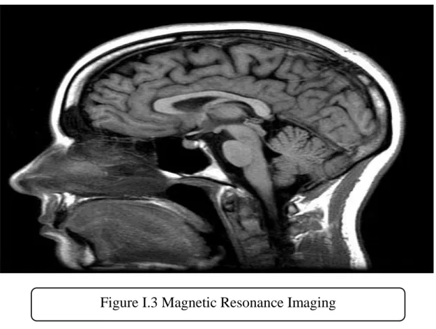
Figure I.3 Magnetic Resonance Imaging ... 9
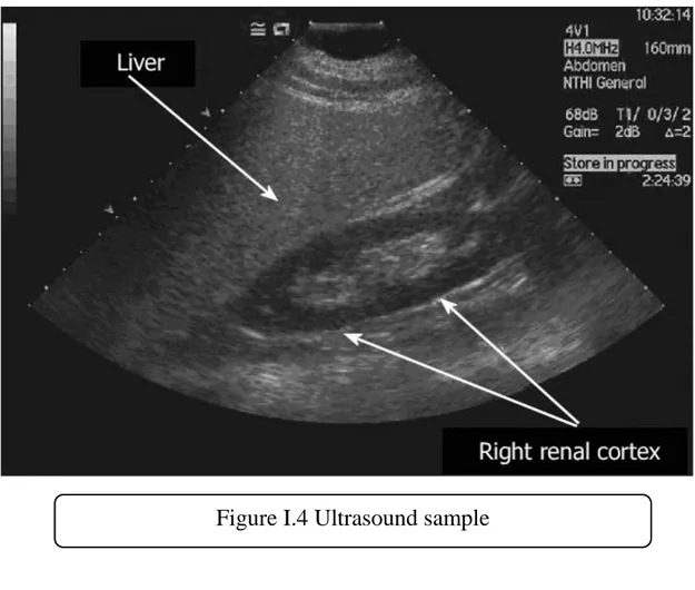
Figure I.4 Ultrasound sample ... 10
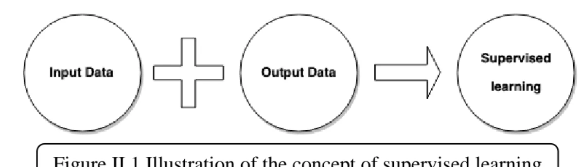
Figure II.1 Illustration of the concept of supervised learning ... 12
Figure II.2 Illustration of the concept of unsupervised learning ... 13
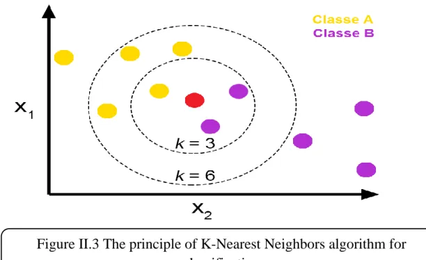
Figure II.3 The principle of K-Nearest Neighbors algorithm ... 15
Figure II.4 Illustration of the concept of Support Vector Machine ... 16
Figure III.2 Bleu and white pictures-same color profile ... 25
Figure III.3 Feature Selection Methods. ... 27
Figure III.4 Blueprint of Filter Method. ... 27
Figure III.5 Blueprint Of Wrapper Method. ... 28
Figure III.6 Blueprint of Embedded Methods. ... 29
Figure IV.1 Architecture of CBIR system ... 31
Figure IV.2 General Architecture ... 32
Figure IV.3 Different types of features ... 33
Figure IV.4 Mechanism of GLCM features ... 34
Figure IV.5 General architecture of feature selection phase ... 39
Figure IV.6 Illustration of the forward selection method ... 40
Figure IV.7 Illustration of the backward selection method ... 41
Figure IV.8 Illustration of the exhaustive selection method ... 42
Figure V.1 Chest X-Ray pneumonia semples ... 42
Figure V.2 Examples of the images contained in ALL-IDB1. ... 43
Figure V.3 illustrate pre-processing phase ... 46
Figure V.4 Chest X-Ray pneumonia samples ... 44
Figure V.5 Examples of the images contained in ALL-IDB1 ... 44
Figure V.6 Illustration of pre-processing phase ... 48
List Of Tables
Table IV.1 Mathematical Equations of Extracted GLCM Features ... 34Table IV.2 Extracted region properties with definition ... 38
Table V.1: Size of disease images ... 45
Table V.2: Illustration of Evaluation scales . ... 47
Table V.3: The range of all involved features ... 48
Table V.4: Results of all features ... 48
Table V.8: Results of classification after feature selection ... 52
List Of Charts
Chart V.1: Classification of features by type ... 49 Chart V.2: Rating results before the selection process ... 51
ML: machine learning
CSV: Comma-Separated Value KNN: K-Nearest Neighbor SVM: Support Vector Machine SFS: Step Forward Selection SBS: Step Backward Selection EXHS: Exhaustive Selection
GLCM:Gray Level Co-Occurrence Matrix RFE:Recursive Feature Elimination
GBM: Gradient boosting machine LR:Linear Regression
NN: Neural Networks LC: Leukemia Cancer NX: Nih X-ray
General Introduction
Years ago and thanks to the new telecommunication and information techniques, medical data became abundant and easy to obtain. However, examining such amount of data is sophisticated and consumes a lot of time. Due to that, using state-of-the-art powerful artificial intelligence techniques like for example Machine Learning (ML), and as science moves a step further, the researcher should not have enough with only reaching a true result but to keep improving either by providing the same results with a lower cost or even getting them better, and why not doing both.
To serve this new purpose, multiple ML branches merged such as Feature Classification, Feature Extraction, selecting suitable appropriate features for every task, Model Evaluation and so many other procedures that sit on pre-provided data and gives back new tools that serve science and knowledge.
We are trying to catch up with their evolution a little bit. We can think of different learning techniques: supervised learning, unsupervised, semi-supervised and others in this thesis. We will principally talk about supervised learning, more specifically, trying to train the computer on a given data and then retrain it on the data output (that is why it is called supervised, we supervise on learning based on data output). Through learning, the computer builds some relationships and patterns between data and its output, hence predicts other data output based on that.
Particularly, we can define our work in three parts: Part One: Extracting features from medical images.
It is a "reducing dimension" operation for transforming data into a simpler shape which represents "raw data".
Part Two: Selecting suitable features from the extracted features in order to optimize classification tasks.
We will mainly apply K-Nearest Neighbor (KNN) algorithm as a learning algorithm. The algorithm KNN coupled with selection methods work on clipping useless features, which helps to reduce the complexity
of the classification task. The final goal is a faster calculating model with a smaller or null prediction error.
Part Three: Classifying images based on selected features.
This study in the first place is a part of treating big bases, speed-up mechanisms, and especially memory management, which makes it very important. Brief, this raises two questions: (1) what level of importance do feature extraction and selection procedures deserve before classifying? (2) Is there an obvious difference between KNN and any other classifiers when dealing with medical images?
Organization: Our work is divided into five chapters: Chapter One
We will talk about medical imaging, its history, its types, and other details.
Chapter Two
We will go through Machine Learning fundamental concepts and its fields of application. We will also talk about classification algorithms. Chapter Three
We will talk about features and processing them. Chapter Four
This chapter is devoted to the presentation of the proposed solution. We will present the global scheme and explain every step.
Chapter Five
We will present the results obtained by our model on three selected large datasets. We analyze and evaluate our results, and eventually compare them with other results.
I.1 Introduction
Since the introduction of medical imaging in the early 20th century, medicine field has changed as a result of the use of precision diagnosis and reduction of unnecessary surgical intervention rates.
Regardless of the technical background, a large number of people heard about medical imaging techniques and many may know some information about their uses, but everyone shares the sense of the importance of these techniques and is impressed by the scientific progress that has reached them. This first chapter is dedicated to presenting the main technologies in medical imaging, namely X-ray, Computer Tomography, Magnetic Resonance Imaging, and Ultrasound.
I.2 Medical imaging
Medical imaging alludes to the methods and procedures used to make pictures of the human body (or parts thereof) for different clinical purposes, for example, surgeries and diagnosis or medical science including the study of normal anatomy and function [1]. In the more extensive sense, it is a piece of natural imaging and joins radiology, endoscope, thermograph, medical photography, and microscopy.
Measurement and recording techniques, for example, electroencephalography (EEG) and magneto encephalography (MEG) are not basically intended to capture pictures but rather which provide information vulnerable to be spoken to as maps, can be viewed as types of medical imaging [2].
I.3 Types of medical imaging I.3.1 Chest X-ray
Chest X-ray utilizes an extremely little portion of ionizing radiation to create photos of within the chest. It is utilized to assess the lungs, heart and chest divider and might be utilized to help diagnose shortness of breath persistent
cough, fever, chest pain or injury. It also may be used to help diagnose and monitor treatment for an assortment of lung conditions, for example, pneumonia, emphysema and cancer. Since chest X-ray is quick and simple, it is especially valuable in emergency diagnosis and treatment [3].
I.3.1.1 Chest X-ray (Chest Radiography)?
The chest X-ray is the most usually performed indicative X-ray examination. A chest X-ray produces pictures of the heart, lungs, aviation routes, veins and the bones of the spine and chest. X-ray (radiograph) is a noninvasive medicinal test that enables doctors to diagnose and treat ailments. Imaging with X-rays includes uncovering a piece of the body to a little portion of ionizing radiation to create photos of within the body. X-rays are the most seasoned and most often utilized type of medical imaging [3].
I.3.1.2 Some basic employments of X-ray
The chest X-ray is performed to assess the lungs, heart and chest divider. A chest X-ray is normally the primary imaging test used to help diagnose side effects, for example: Breathing difficulties, a bad or persistent cough, chest pain or injury, fever.
Physicians use the examination to help diagnose or monitor treatment for conditions such as: Pneumonia, heart failure and other heart problems, emphysema, lung cancer, positioning of medical devices, fluid or air collection around the lungs, other medical conditions [3].
I.3.1.3 How does the X-ray work?
X-rays are a type of radiation like light or radio waves. X-rays go through most articles, including the body. When it is painstakingly gone for the piece of the body being inspected, a X-ray machine delivers a little burst of radiation that goes through the body, recording a picture on photographic film or an
extraordinary locator. Various pieces of the body retain the X-rays in fluctuating degrees. Thick bone assimilates a significant part of the radiation while delicate tissue, for example, muscle, fat and organs, permit a greater amount of the X-rays to go through them. Thus, bones seem white on the X-ray, delicate tissue appears in shades of dark and air seems dark. On a chest X-ray, the ribs and spine will assimilate a great part of the radiation and seem white or light dark on the picture. Lung tissue retains little radiation and will seem dim on the picture. Five essential densities are perceived on plain radiographs (Figure I.1), listed here in order of increasing density:
1. Air/gas: black, e.g. lungs, bowel and stomach;
2. Fat: dark grey, e.g. subcutaneous tissue layer, retroperitoneal fat;
3. Soft tissues/water: light grey, e.g. solid organs, heart, blood vessels, muscle and fluid-filled organs such as bladder;
4. Bone: off-white;
5. Contrast material/metal: bright white.
Up to this point, x-ray pictures were kept up on huge film sheets (much like an enormous photographic negative). Today, most pictures are computerized documents that are put away electronically. These put away pictures are effectively available for finding and malady the executives [3].
I.3.1.4 Advantages versus dangers Advantages:
No radiation stays in a patient’s body after a X-ray examination.
X-rays more often than not have no reactions in the common symptomatic range for this test.
X-ray hardware is generally reasonable and broadly accessible in crisis rooms, doctor workplaces, mobile consideration focuses, nursing homes and different areas, making it advantageous for the two patients and doctors.
Since x-ray imaging is quick and simple, it is especially valuable in crisis analysis and treatment.
Dangers:
Excessive exposure to radiation. However, the benefit of an accurate diagnosis far outweighs the risk.
The powerful radiation portion for this strategy varies.
Women should always inform their doctor or X-ray technologist if there is any probability that they are pregnant [3].
I.3.2 Computer Tomography (CT)
Computer tomography (CT) or ‘Feline’ scans are a type of X-ray that makes a 3D picture for determination. CT or figured hub tomography (CAT) uses X-rays to deliver cross-sectional pictures of the body. The CT scanner has a huge round opening for the patient to lie on a mechanized table. The X-ray source
and an identifier at that point turn around the patient delivering a tight ‘fan-molded’ light emission ray that goes through an area of the patient’s body to make a preview.
These depictions are then examined into one, or different pictures of the inside organs and issues.
CT examines give more noteworthy lucidity than traditional X-rays with increasingly point by point pictures of the interior organs, bones, delicate tissue and veins inside the body.
The advantages of utilizing CT examines far surpass the dangers which, as with X-rays, incorporate the danger of cancer, mischief to an unborn youngster or response to a complexity operator or color that might be utilized. In numerous cases, the utilization of a CT filter averts the requirement for exploratory surgery.
It is significant that when checking youngsters, the radiation portion has been brought down than that utilized for grown-ups to forestall an absurd portion of radiation for the vital imaging to be gotten. In numerous medical hospitals you’ll locate a pediatric CT scanner thus [6].
I.3.3 Magnetic Resonance Imaging (MRI)
MRI scans create diagnostic images without using harmful radiation, Magnetic Resonance Imaging (MRI) uses a solid magnetic field and radio waves to create pictures of the body that can’t be seen well utilizing X-rays or CT filters, for example it empowers the view inside a joint or tendon to be seen, instead of only the outside [5].
MRI is generally used to look at interior body structures to diagnose strokes, tumors, spinal rope wounds, aneurysms and mind work.
As we probably am aware, the human body is made for the most part of water, and each water atom contains a hydrogen core (proton) which winds up adjusted in a magnetic field. An MRI scanner utilizes a solid magnetic field to adjust the proton ‘turns’, a radio recurrence is then connected which makes the protons ‘flip’ their twists before coming back to their unique arrangement [7].
Protons in the distinctive body tissues come back to their typical twists at various rates so the MRI can recognize different kinds of tissue and distinguish any variations from the norm. How the atoms ‘flip’ and come back to their ordinary turn arrangement are recorded and prepared into a picture [7].
MRI doesn’t utilize ionizing radiation and is progressively being utilized amid pregnancy with no reactions on the unborn kid detailed. However, there are dangers related with the utilization of MRI scanning and it isn’t prescribed as a first stage finding [5].
I.3.4 Ultrasound
Ultrasound is the most secure type of medicinal imaging and has a wide scope of uses. There are no unsafe impacts when using ultrasound and it’s a standout amongst the most practical types of restorative imaging available to us, paying little heed to our claim to fame or conditions [5].
Ultrasound utilizes sound waves rather than ionizing radiation. High-recurrence sound waves are transmitted from the test to the body by means of the leading gel, those waves at that point ricochet back when they hit the various structures inside the body and that is utilized to make a picture for diagnosis.
Another kind of ultrasound regularly utilized is the ‘Doppler’ – a somewhat extraordinary system of utilizing sound waves that permits the blood course through supply routes and veins to be seen.
Due to the minimal danger of utilizing Ultrasound, it’s the principal decision for pregnancy, yet as the applications are so wide (crisis conclusion, cardiovascular, spine and inward organs) it will in general be one of the primary ports of call for some patients [8].
I.4 Conclusion
Rapid advances in medical science and the invention of sophisticated detection devices have benefited mankind and civilization. Modern science also changed the medical field. This has led some to say that artificial intelligence may someday replace human radiation experts, so researchers have developed the machine to learn or so-called machine learning as they have developed neural networks of deep learning, the correct diagnosis of diseases is the essential necessity before treatment. The more dynamic the tools are, the better the diagnosis will be. In the next few years we will see some of the methods and techniques that will contribute significantly to the identification of pathogens in radiological images. One day artificial intelligence may in some cases be more reliable than the normal radiologist.
II.1 Introduction
Solving a problem by programming consist in establishing a set of sequences of instructions to be performed on inputs to return outputs. These programs represent algorithms that have the ability to solve so many problems including difficult mathematics equations, graph problems, optimization problems, and so on . But, today, we have problems such as, Spam filtering, Face recognition, Machine translation, Speech recognition, etc., that need more sophistical algorithms for their solution. Large number of such problems can be solved with machine learning (ML). ML algorithms find certain patterns in large datasets and build consistent rules to make future predictions or to make decisions.
II.2 Machine Learning
ML is one of several artificial intelligence domains which focus on designing algorithms that allows the computers to "learn", without programming the logic (rules) for each problem. ML can be seen as child learning since his birth to gradually recognizing things and sounds by guiding him and correcting his information, and repeating the process till he learns. The principle is the more guiding and information we provide, the more knowledge and experience we acquire. A child learns either by his parent supervision or by getting exposed directly to an event, for gaining the experience.
II.2.1 Classification Techniques
II.2.1.1 Supervised Learning
Computers are trained by the given data and their outputs (that’s why it's called supervision; we supervise the learning by giving the outputs of the data), and by learning the computer build relations and patterns
between the data and the outputs, so as it can later predict the outputs for new data [9].
II.2.1.1.1 Classification
The classification problem is referring to a function that returns a discrete variable from input variables. The output is called label or
category. For example, the problem of ‘dog or cat’ is classification
problem.
II.2.1.1.2 Regression
For a regression problem the function return continues variable from the input variables, for example a linear regression to predict the prices of products.
II.2.1.1.3 The difference between two types: What is the temperature going to be tomorrow?
Prediction for classification is: hot or cold.
Prediction for regression is temperature value for example 84 degree.
II.2.1.2 Unsupervised Learning
Computers are trained by only the given data (that's why it's called unsupervised, where we don't supervise the learning and we don't give the outputs of the given data), and by learning the computer build relations
and patterns between the data itself so it can predict the outputs of the data [9].
II.3 Machine Learning Usage
Recognizing and identifying things (face, images, character, words, texts, sounds, music, etc.)
Helping to find medics to heal infectious diseases and recognizing diseases
Search engines and information security and marketing answering questions (information bank)
Making decisions and recommendations by simulating humans neural networks
Anticipating in developing robots to do different tasks and specially difficult and exact tasks for humans
II.4 Machine Learning Algorithms
ML is an ensemble of programs that is putted in general rules and forms to treat the inputs data of all forms, and find relations and patterns in the data, by applying statistical and mathematical equations. Each algorithm is characterized by specific features and outputs, to be able to represent data in different ways or predict outputs for new data, based on the relations and the patterns extracted from the input data.
II.4.1 K-Nearest Neighbor (KNN) II.4.1.1 KNN for classification
The KNN is the most fundamental and the simplest classification technique when there is little or no prior knowledge about the distribution of the data . This rule simply retains the entire training set during learning and assigns to each query a class represented by the majority label of its k-nearest neighbors in the training set. The Nearest Neighbor rule (NN) is the simplest form of KNN when K = 1.
In KNN, each sample should be classified similarly to its surrounding samples. Therefore, if the classification of a sample is unknown, then it could be predicted by considering the classification of its nearest neighbor samples. All the distances between the unknown given sample and all the samples in the training set can be computed [3]. The distance with the smallest value corresponds to the sample in the training set which is the closest to the unknown sample. Therefore, the unknown sample may be classified based on the classification of this nearest neighbor .
Figure II.3 shows the KNN decision rule for and for a set of samples divided into 2 classes. With , an unknown sample is classified by using only two neighbors, when more than two neighbors is used. In the last case, the parameter is set to , so that the closest six neighbors are considered for classifying the unknown sample. Four of them belong to the same class, whereas two belongs to the other class. [11]
II.4.1.2 Advantages and Disadvantages II.4.1.2.1 Advantages
The algorithm KNN has several main advantages: simplicity, effectiveness, intuitiveness and competitive classification performance in many domains. It is robust to noisy training data and is effective if the training data is large. Also the training cost is equal to 0 and it is stable and strong when it comes to the noises of data. Also efficient with big data and it doesn’t have to make any hypothesis about the concept features that it has to learn.
II.4.1.2.2 Disadvantages
The calculations are heavy;
The performance depends on the number of dimensions;
We must know the factor .
Figure II.3 The principle of K-Nearest Neighbors algorithm for classification
II.4.2 Support vector machine (SVM)
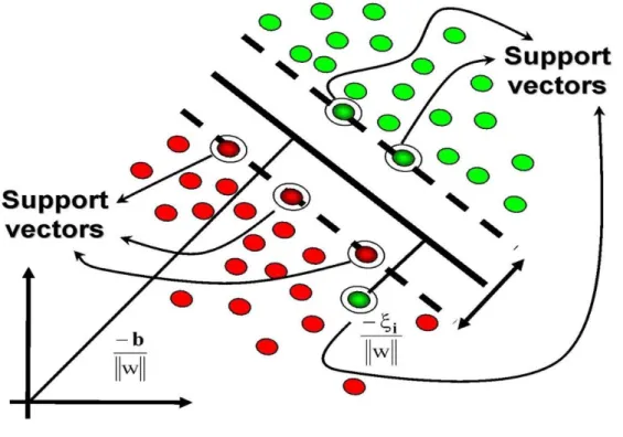
SVM is a supervised machine learning algorithm. It is classification and regression algorithm, used mostly on classification problems. In SVM, we draw every data element as a point in the n-dimensional space (where is the features) with the value of each feature is the value of a specific coordinate.
The concept SVM refers to the maximum limit that separates a specific class from the other classes. If two classes are well separated from each other, then it is easy to find the support vector machine [10].
II.4.2.1 Advantages
A robust classification algorithm;
Good performance with a clear separation margins;
Efficient on the high dimensional spaces;
One of the most best algorithms in the training data;
Efficient in the situation where the number of dimensions is bigger than the number of samples;
Doesn’t make any strong hypothesis on the data. II.4.2.2 Disadvantages
It doesn't perform well when:
We have big data, because the training time is very high;
When the ensemble of data has a lot of noise, the targeted classes overlapping;
It doesn't provide a direct probability evaluation.
II.4.3 Random Forest
Random Forest is considered as the best way for solving problems in data analyzing. There’s a proverb that says ‘when you can't think of an algorithm (no matter what the problem is) use Random forest’, which is a term for an ensemble of decision trees called 'forest'. In the Random Forest we create several trees rather than one single tree for classifying a new object based on the features. Each tree gives a classification, and we say that the tree a 'vote' for that class. The forest chooses the class that has the large number of votes (of all the trees in the forest). For regression case, it takes the average of all results depending on the different trees. It considered as a machine learning algorithm with several usage for classification and regression problems, as it takes techniques of dimensions reducing, and it can treat the missing and the outsider values, and the other essential steps for data explorations.
II.4.3.1 Advantages
Random Forest technique,
can solve both of the classification and regressions problems;
has the power of treating a big data with a larger dimensions;
has an effective way to estimate the missing values, and reserves the accuracy when it misses a large amount of data;
has methods for errors balancing in the data groups where the classes are unbalanced.
II.4.3.2 Disadvantages
Random Forest is certain that it does a good job for classification but not as good as the prediction problem because it doesn't give an exact continuous natural prediction. Random Forest may appear like a black box for the statistical model designers; you have a little control on what the model do.
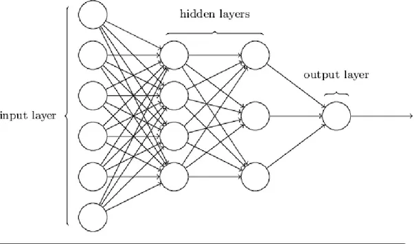
II.4.4 Neural Networks
Neural Networks are techniques designed to simulate the way the human brain perform a certain task in distributed and parallel manner. It is composed by simple processing units, which is only just calculating elements called nodes or neurons. IT has a Nervous property, for storing the Practical knowledge and the experimented information, and making them available for the .
Neural Networks are trained by setting the weights in the nodes and passing the input values to the other successive layers to emerge the results [10].
II.4.4.1 Advantages
The most known and used algorithm in machine learning and deep learning;
Simple and fast technique with the availability of the different training algorithms;
The ability to detect the inner nonlinear complex relations between the independent variables and the ability to detect most of the possible interactions between the predictions variables.
II.4.4.2 Disadvantages
It needs intensive calculations and high-end computers
Selecting the structure of the proper networks is a challenge
Sometimes there's unexplained behavior of the network and it is hard to follow the networks and correct it.
II.5 Application domains
Both feature extraction and selection play an important role in every multi-dimensional statistical task. There are a lot of application fields including finance, security, cars manufacture and technology in general. To mention some examples, there is Watson fusion in cancer memorial center (Sloan Kettering New York). Self-driving cars which is the most representative and led by Google. Speech, facial and entity recognition in security and information. It is Artificial Intelligence that depends on a colossal database to create more modern medical diagnosis with less time and cost comparing to human specialists even the highly skilled. Discovering finance fraud or DNA frequency all of them fall under Automatic Learning aspect.
II.6 Conclusion
What should be remembered from all of this is simply that artificial intelligence seems to promise a bright future, given the technological reach of machine learning. The learning machine offers a number of advanced statistical methods to deal with regression and classification functions with many different and independent variables. Among these methods, let's mention the SVM (support Vector Machine) for regression and classification problems, the Naive Bayesian Networks method for solving classification problems, and the methods of KNN (K-nearest neighbors) for regression and classification problems.
III.1 Introduction
For many years, data analysis has been a vast area of research for many researchers. Due to the vast amount of data and information available in the databases, strong techniques and tools are needed for better handling data and extracting related knowledge.
It is crucial that we examine machine learning pipeline before proceeding with feature engineering as to have a better idea about the application. Consequently, we will encounter and reflect upon some concepts like tasks and models and data.
III.2 Data
Data resembles information observed in real life. For example, the data on global economy may include, but are not limited to, the observation of the continuous shifts in prices of goods, rate of profit made by shareholders in stock market, and so on. Medical history should include information about previous medications and medical cases the individual has undergone. It may include rates of blood pressure, epinephrine injection prescriptions, and notes on allergies. These are only examples from different fields. The extent to this reaches every aspect of our lives.
Data is like a piece from a puzzle board that joins with many other pictures to create a coherent image. But no image is perfect, and this suggests and indicates that there are always some intervals and overlaps between data that make credibility questioned and sought to be proved in order to gain validity [13].
III.3 Tasks
There are many reasons that justify the collection of data. Data can be the answer to many question we have as they demonstrate certain facts pertaining a specific idea like “Which cryptocurrency should I use?” or “How do I make advertisement more efficient ?”
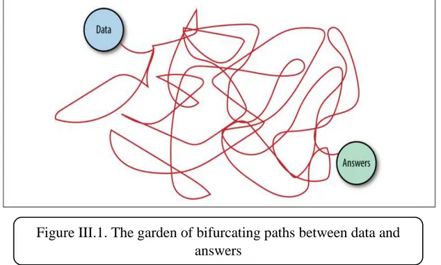
It is easy to decide which approach is better to take in order to reach a certain destination as far as data is concerned (see Figure III-1). Sometimes, luck and chance may roll the dice and the worst possible approach to ever imagine becomes the one leading to highly successful results [13].
III.4 Models
Understanding reality by means of data is a chaotic process that is not error-free. In order to set it straight, mathematical modeling, especially in statistical modeling, becomes very handy. Statistics are characterized by having some form of frequency in data.
These data are labeled conceptionally according to their nature such as wrong and redundant data, which implies the occurrence of a mistake in the process of measurement and self-evidency on various levels, respectively. For example, a month can exist as a categorical variable. The values of the possible variants are “March,” “April,” “May,” and so on, and then included as integer values in the range [0, 11]. When a certain month does not appear for some data points, then the some data is missing.
Figure III.1. The garden of bifurcating paths between data and answers
The different aspects of data are explained through the mathematical model. For example, a model that predicts real estate revenues may be a formula that highlights a firm’s earning history.
Mathematical formulas relate numeric quantities to each other. But raw data is often not numeric (The action “Alice bought The Lord of the Rings trilogy on Wednesday” is not numeric, and neither is the review that she subsequently writes about the book). There must be a piece that connects the two together; this is where features come in [13].
III.5 Features
Features are the numeric embodiment for raw data. There are countless ways to make raw data numeric. Features need to be extracted from available types of data. They are connected to the model, and so there is a reciprocal relationship of appropriateness between models and types of features. The appropriateness of features is based on task-relevancy and simplicity of process; and as such, its structure is based on these two aspects in respect to the task.
Moreover, the number of features represents their informative capacity which is later translated itself as the competence to fulfil the task [13]. However, having an excess of features would increase the cost of the model and make it harder to be trained and it is very probable that something could go wrong in the process .
III.6 Image features
There is a huge difference in mastering some of the skills that we think of as axiomatic. For instance, processing visual and auditory stimuli is innate in the sense that it does not need a special training to master and comes as a result of the unique neuro sensory system of human beings. In contrast, language learning and language skills are developed by means of social interaction and accumulation of experience.
As machine learning could be described more or less as the artificial clone of the human brain, one would expect the same scenario to take place. Interestingly, the situation is completely the opposite. We have been far more successful in analyzing texts than we could ever dream of as opposed to visuals and audios. It is crystal clear that, while searching, the success in obtaining information comes at an incredible ease and timely fashion while dealing with texts compared to visuals and audios.
Difficulty of extracting meaningful features and difficulty of progress are inseparable. Machine learning models require meaningful semantics in order to produce accurate predictions. That is one of pros of searching in English as words in the English language have the capacity to shift between grammatical units while maintaining the same semantic significance, which is translated in the speed of searching.
On the other hand, visuals and audios are made of pixels. That is smallest unit within their frames. It is the case that these pixels offer no semantic significance, hence the difficulty in analyzing these formats.
Twenty years ago, SIFT and HOG were the standards for extracting good visual features. The recent development in deep learning research has successfully implemented auto feature extraction in the basic substrata. What happens is: when manually defined feature (which were used in SIFT and HOG, fundamentally) is replaced with manually defined models, a better performance in extracting features is achieved. This by no means eliminates the manual work; it just sets it one step apart from modeling.[13]
III.7
Impracticality of simple image features
Extracting features from visuals, an image per se, depends on the aim one needs them for. For instance, if one is to restore a picture from a certain data base, then it is important to find a way with which to present all the images in
the database. And not only that, it is also imperative to find a way to distinguish between them. Color may be a way to do that, but it is not enough because some images may have the same colors roughly but they represent completely different things.
Are the percentages of colors in the image sufficient?
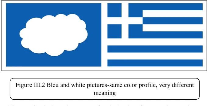
Figure 8-1 presents two images that roughly have the same color profile but very different meanings; one represents a cloud in the sky, and the other represents the Greek flag, respectively. Thus, colors alone are insufficient to characterize an image.
We can also look at the contrast in pixel values between the two images. Firstly, the images must have the same size, if they’re not, resize is required. A matrix of pixel values would represent both pictures. A long vector can contain a matrix, either by row or by column.
The feature of the image is now represented through the color of the pixel (RGB encoding). Finally, it measures the Euclidean distance between the long pixel vectors. This would definitely allow us to tell apart the Greek flag and the white clouds, but it is too stringent as a similarity measure.
Figure III.2 Bleu and white pictures-same color profile, very different meaning
A cloud could take on a thousand different shapes and still be a cloud. It could be shifted to the side of the image, or half of it might lie in shadow. All of these transformations would increase the Euclidean distance, but they shouldn’t change the fact that the picture is still of a cloud [13].
The problem is that individual pixels do not carry enough semantic information about the image. Therefore, they are bad atomic units for analysis.
III.8
Feature ExtractionFeature extraction methodologies analyze objects and images to extract the most prominent features that are representative of the various classes of objects. Features are used as inputs to classifiers that assign them to the class of image that they represent. Here is a small defibtion of texture and shape features
III.8.1 Texture features
The texture feature is extracted usually using filter base method. The Gabor filter (Turner, 1986) is a frequently used filter in texture extraction. A range of Gabor filters at different scales and orientations captures energy at that specific frequency and direction. Texture can be extracted from this group of energy distributions (Mulleret al., 2004). Other texture extraction methods are co-occurrence matrix, wavelet decomposition, Fourier filters, etc [17].
III.8.2 Shape features
Shape is an important and powerful feature for image classification. Shape information extracted using histogram of edge direction. The edge information in the image is obtained by using the Canny edge detection (Canny, 1986). Other techniques for shape feature extraction are elementary descriptor, Fourier descriptor, template matching, etc [16].
III.9
Feature SelectionFeature Selection methods are used to remove nonuseful features to reduce the complexity of the that we will have later , the final goal is to get a model that use the minimum resources , faster in time to calculate and with deduction or at the least no degradation in the Accuracy [13].
To have such a model in hand , there’s a selection methods that train more than one candidate model , the purpose of feature selection is not isn’t reducing model training time , but to reduce model scoring time .
Multivariate Feature Selection is broadly divided into three categories:
III.9.1 Filter method
Filtering methods are more like preprocessing method that removes features that maybe unusual for the model, one could compute the correlation or mutual information between each feature and the response variable, and filter out the features that fall below a threshold, filtering methods far less costing than the wrapper methods, but they don’t take into account the model that you will use, so they may remove the right features for the model [13].
III.9.2 Wrapper method
Wrapper methods are expensive, because you can create multiple models with multiple subsets of features. They will prevent you from removing useful features that are bad to use in your model by themselves but good to be in the model in combination. Wrapper methods handle the classifier or regressor as a black box algorithm that gives a decent accuracy of a given subset of features [13].
We decide if we are going to add a feature or remove it from our subsets depending on the results of our past model.
They are named wrapper methods because they wrap a classifier model up in a feature selection search method. First a set of features will be chosen then depending on the perturbation and efficient changes will be made.
The main negative thing about this method that is it takes a large amount of times and computation that makes it expensive, because if the feature
Figure III.4 Blueprint of Filter Method [15].
space is vast which is quite often, the method will be looking at every possible combination.
III.9.3 Embedded methods
Embedded methods incorporate feature selection as part of the model training process. They are not as powerful as wrapper methods, but they are nowhere near as expensive. Compared to filtering, embedded methods select features that are specific to the model. In this sense, embedded methods strike a balance between computational expense and quality of results.
III.10 Conclusion
No matter what is the data we want process, the features are the key to how good a machine learning model is, especially when dealing with images. If a set of inappropriate features is extracted, the model's predictions will be inaccurate and unreliable. So we have to choose the best set of features that is compatible and represent our dataset in a correct way to provide accurate and reliable results. In the next chapter we will present the proposed solution in our study and how to use the methods of extraction and selection.
IV.1 Introduction
Scientists found many problems in diagnosing medical images either because of many diagnostic requests or the difficulty of diagnosis itself. Here, artificial intelligence intervenes to solve the problem because traditional algorithms no longer solve these problems. Artificial intelligence or Machine learning also provide a powerful addition in medical fields and help the doctors and their patients together.
In this chapter, we present our proposed solution that based on machine learning techniques. We begin by presenting related works and the general architecture.
Images have a very large number of features. In this chapter, we provide different types of features from medical images. We define them and explain how to extract them.
Features are an important element in image classification as they provide information that contributes to the good classification of images. Since not all features are important, we address the feature selection step using the KNN algorithm (as it is one of the simplest algorithms in machine learning) coupled with other selection methods.
IV.2 The most important classification problems and contributions
of others in solving them
There are hardly many problems faced by the researchers and the developers in data analysis, especially in medical fields. Among these problems are those related to extracting features from images. There are several questions about what type of dataset to deal with and what type of medical imaging they have undergone, what characteristics should be chosen? Are these features really useful for the disease
you are going to diagnose? Each disease has its own model, which is different from other diseases. Other problems related to identifying the important features. What is the effective way to identify important features? Especially with different features affecting training and learning for the model, as well as classification problems, what is the appropriate algorithm to be applied to give satisfactory, reliable and accurate results [16].
IV.2.1 Previous works
A growing trend in the field of image retrieval is automatic classification of images by different machine learning classification methods. Image retrieval performance depends on good classification, as the goal of image retrieval is to return a particular image from class according to the features provided by the user (Lim et al., 2005). The most common approach in content-based image retrieval is to store images and there feature vector in a database. Similar images can be retrieved from database by measuring the similarity between the query image features and database features space as shown in Fig. IV.1, the general architecture of CBIR system proposed by Lehmann et al. (2000). Kherfi et al. (2004) pointed out in his survey review many of the system used this approach, such as QBIC (Flickner et al., 1995) was proposed by IBM, Photobook (Pentland et al., 1996) and BlobWorld (Carson et al., 1999) proposed from academic circles. These systems not being able to classify images in particular group they just retrieved similar images from the database.
This limitation brings researchers into research of classifying images according to particular categories (Kherfi et al., 2004). In medical domain CBIR is facing same problem. Medical images play a central part in surgical planning, medical training and patient diagnoses. In large hospitals thousands of images have to be managed every year (Mulleret al., 2004). Manual classification of medical images is not only expensive but also time consuming and vary person to person [16].
IV.3 General Architecture
Figure IV.1 Architecture of CBIR system [16]
The general architecture describes the steps that make up the project and it is illustrated in Figure IV.2.
After we have received the images we begin by preparing dataset for easy handling, and then we move to the stage of extracting features that are very important in images generally and medical images specifically. The phase of selecting features which is the most important phase for which we will use the KNN algorithm in order to select the most suitable features that reduces the computational time to train our models and leads to more accurate classification.
IV.4 Feature extraction
At this phase, the input is raw medical images. Two fundamental types of features: texture features and shape features. For the first type we use GLCM features, and for the second type we use the region and moments features. The output is Numerical values of different dimensions. These features are the most common features in the analysis and recognition of patterns in medical images.
IV.4.1 GLCM Features
Texture contains important information regarding underlying structural arrangement of the surfaces in an image. Gray level co-occurrence matrix (GLCM) is well-known texture extraction features originally introduced by Haralick et al. (1973).
The GLCM is constructed by getting information about the orientation and distance between the pixels. Many texture features can be extracted from this GLCM (Acharya, 2005). For this task four GLCM matrixes for four different
Figure IV.4 Mechanism of GLCM features [17]
Table IV.1 Mathematical Equations of Extracted GLCM Features
Energy feature Correlation feature
contrast feature Pij 1 + i − j 2 N−1 ij=0 Homogeneity feature feature 𝑃𝑖𝑗 ⅈ − 𝑗 2 𝑁−1 𝑖,𝑗=0 𝑃𝑖𝑗 𝑖 − 𝑢 𝑗 − 𝑢 𝜎2 𝑁−1 𝑖,𝑗=0 𝑃𝑖𝑗 ⅈ − 𝑗 2 𝑁−1 𝑖,𝑗=0
orientations (0°, 45 °, 90°, 135°) are obtained. Several texture measures may be directly computed from the GLCM (Haralick et al., 1973). We computed Contrast, Energy, Homogeneity, and Entropy from each image [17].
Where:
=is the variance of the intensities of all reference pixels in the relationships that contributed to the GLCM ,calculated as [17]:
=is the element i j of the normalized symmetrical GLCM.
=is the number of gray levels in the image as specified by Number of levels.
=is the GLCM mean (being estimate of the intensity of all pixels in the relations that contributed to the GLCM),calculated as:
IV.4.2 Shape Features
Shape provides geometrical information of an object in an image, which do not change even when the area, scale and orientation of the object are changed. In this project we will use Hu Moments and moment and Region features.
Hu Moments (or rather Hu moment invariants) are a set of 7 numbers calculated using central moments that are invariant to image transformations. The first 6 moments have been proved to be invariant to translation, scale, and rotation, and reflection. While the 7th moment’s sign changes for image reflection [21].
𝜎2 𝜎2 = 𝑃 𝑖𝑗 ⅈ − 𝑢 2 𝑁−1 𝑖,𝑗=0 𝑃𝑖𝑗 𝑁 𝑢 𝑢 = ⅈ𝑃𝑖𝑗 𝑁−1 𝑖,𝑗=0
IV.4.2.1 Moments
Image moments are used to describe objects and play an essential role in object recognition and shape analysis. Images moments may be employed for pattern recognition in images. Simple image properties derived via raw moments is area or sum of grey levels [18].
Central Moments are defined by:
Central Moments of order up to 3 are:
Information about image orientation can be derived by first using the second order central moments to convert moment to construct a covariance matrix. Its specific definitions are as follows:
𝑢𝑃𝑞 = 𝑥 − 𝑥 𝑝 𝑦 − 𝑦 𝑞𝑓 𝑥, 𝑦 𝑦 𝑥 𝑢00 = 𝑀00, 𝑢01 = 0, 𝑢10 = 0, 𝑢11 = 𝑀11 − 𝑥𝑀01 = 𝑀11 − 𝑦𝑀10, 𝑢20 = 𝑀20 − 𝑥𝑀10, 𝑢02 = 𝑀02 − 𝑦𝑀01, 𝑢21 = 𝑀21 − 2𝑥𝑀11 − 𝑦𝑀20 + 2𝑥2𝑀01, 𝑢12 = 𝑀12 − 2𝑦𝑀11 − 𝑥𝑀02 + 2𝑦2𝑀10, 𝑢30 = 𝑀30 − 3𝑥𝑀20 + 2𝑥2𝑀10, 𝑢03 = 𝑀03 − 3𝑦𝑀02+ 2𝑦2𝑀01, 𝑢20′ = 𝑢20 𝑢00 = 𝑀20 𝑀00 − 𝑥 2 𝑢02′ = 𝑢02 𝑢00 = 𝑀02 𝑀00 − 𝑦 2 𝑢11′ = 𝑢11 𝑢00 = 𝑀11 𝑀00 − 𝑥𝑦
IV.4.2.2 Hu moments
As shown in the work of Hu, invariants that are translation, scale and rotation can be constructed as follows [19]:
These are well-known as Hu moment invariants.
After the partitioning process, we extracted the moments and Hu moments for their importance and need for object recognition and shape analysis and can be used in our project to identify patterns of diseases in medical images.
IV.4.2.3 Region Features
Region feature extractors process square image neighborhoods and represent its central pixel by the resulting feature vector. This is useful to account for local spatial information and structure in images. Typical applications are texture classification and image segmentation (distinguishing edges).
Various region properties features are going to be extracted, they are defined as follows: 𝐼1 = 𝜂20 + 𝜂02 𝐼2 = 𝜂20 − 𝜂02 \2 + 4𝜂112 𝐼3 = 𝜂30 − 3𝜂12 2+ 3𝜂 21− 𝜂03 2 𝐼4 = 𝜂30 − 𝜂12 2+ 𝜂 21 + 𝜂03 2 𝐼5 = 𝜂30 − 3𝜂12 𝜂30 + 𝜂12 𝜂30 + 𝜂12 2− 3 𝜂 21 + 𝜂03 + 3𝜂21− 𝜂03 𝜂21+ 𝜂03 3 𝜂30+ 𝜂12 2− 𝜂 21+ 𝜂03 2 𝐼6 = 𝜂20 − 𝜂02 𝜂30 + 𝜂12 2− 𝜂 21 + 𝜂03 2 + 4𝜂11 𝜂30+𝜂12 𝜂21+𝜂03 𝐼7 = 3𝜂21 − 𝜂03 𝜂30 + 𝜂21 𝜂30 + 𝜂12 2− 3 𝜂 21 + 𝜂03 2 − 𝜂30 − 3𝜂12 𝜂21 + 𝜂03 3 𝜂30 + 𝜂12 2− 𝜂 21 + 𝜂03 2 .
IV.5 Feature Selection
This phase is considered the most important phase in our project. It is a crucial phase for building a proper model. We start with restructuring the numerical values of the extracted features. Then we select the best features for the training and
Definition Name
The longest diameter of an ellipse Of an ellipse
Major axis
The shortest diameter of an ellipse Of an ellipse
Minor axis
Number of pixels of the region will all the holes filled in. Describes the area of the filled_image
filled_area
Inertia tensor of the region for the rotation around its mass inertia_tensor
region Number of pixels of the area
Angle between the 0th axis (rows) and the major axis of the ellipse that has the same second moments as the region, ranging from
-pi/2 to -pi/2 counter-clockwise orientation
Number of pixels of bounding box bbox_area
Region with the maximum area out of all the segmented small chunks max_area
Mean value of area of all the segmented small chunks mean_area
Standard deviation of area of all the segmented small chunks std_area
The eccentricity is the ratio of the distance between the foci of the ellipse and its major axis length. The value is between 0 and 1
eccentricity
The proportion of pixels in the smallest convex polygon that contains the region.
solidity
It is a scalar quantity; equal to the number of objects in the region minus the number of holes in those objects.
euler_number
Simply the perimeter of the region. perimeter
Centroid coordinate tuple (row, col), relative to region bounding box local_centroid
The two eigen values of the inertia tensor in decreasing order.
inertia_tensor_eigvals
The length of the major axis of the ellipse that has the same normalized second central moments as the region.
major_axis_length
The length of the minor axis of the ellipse that has the same normalized second central moments as the region.
minor_axis_length
Number of pixels of convex hull image, which is the smallest convex polygon that encloses the region.
convex_areaint
Ratio of pixels in the region to pixels in the total bounding box. Computed as area /(rows * cols)
extentfloat
The diameter of a circle with the same area as the region.
equivalent_diameter
classification process using different selection methods such as SFS, SBS and EXHS.
The selection of any non-important feature in the prediction process will give us a weak and inaccurate model. Since the principle that the KNN algorithm based on is to choose the nearest neighbor by calculating the distance between all features and the nearest neighbors will be selected to be considered the best features, we have made it an intermediary in the heuristic search methods listed below.
IV.5.1 Selection methods
IV.5.1.1 Forward Selection
Forward selection is an iterative method in which we start with having no feature in the model. In each iteration, we keep adding the feature which best improves our model till an addition of a new variable does not improve the performance of the model.
These steps illustrate the mechanism of how the process of forward selection works:
Predict the labels of the dataset by creating a KNN model for each feature.
Get the one most accurate feature in those models.
Add selected feature to the group .
Create another set of models for the group plus one each feature outside the group.
Add the feature of the best model to the group .
Re-process until get to the number of selected features to be determined. Figure IV.6 Illustration of the forward selection method