HAL Id: hal-02900537
https://hal.archives-ouvertes.fr/hal-02900537
Submitted on 16 Jul 2020
HAL is a multi-disciplinary open access
archive for the deposit and dissemination of
sci-entific research documents, whether they are
pub-lished or not. The documents may come from
teaching and research institutions in France or
abroad, or from public or private research centers.
L’archive ouverte pluridisciplinaire HAL, est
destinée au dépôt et à la diffusion de documents
scientifiques de niveau recherche, publiés ou non,
émanant des établissements d’enseignement et de
recherche français ou étrangers, des laboratoires
publics ou privés.
using the PSQA metric
Gerardo Rubino, Martin Varela, Jean-Marie Bonnin
To cite this version:
Gerardo Rubino, Martin Varela, Jean-Marie Bonnin. Controlling multimedia QoS in the future home
network using the PSQA metric. British Computer Society’s Computer Journal, 2006, 49 (2), pp.137
- 155. �hal-02900537�
Controlling Multimedia QoS in the Future Home
Network Using the PSQA Metric
Gerardo Rubino, Mart´ın Varela and Jean–Marie Bonnin
AbstractHome networks are becoming ubiquitous, especially since the advent of wireless technologies such as IEEE 802.11. Coupled with this, there is an increase in the number of broadband–connected homes, and many new services are being deployed by broadband providers, such as TV and VoIP. The home network is thus becoming the “media hub” of the house. This trend is expected to continue, and to expand into the Consumer Electronics (CE) market as well. This means new devices that can tap into the network in order to get their data, such as wireless TV sets, gaming consoles, tablet PCs, etc. In this paper, we address the issue of evaluating the QoS provided for those media services, from the end–user’s point of view. We present a performance analysis of the home network in terms of perceived quality, and show how our real-time quality assessment technique can be used to dynamically control existing QoS mechanisms. This participates to minimizing resource consumption by tuning the appropriate QoS affecting parameters in order to keep the perceived quality (the ultimate target) within acceptable bounds.
I. INTRODUCTION
Over the last few years, the growth of the Internet has spawned a whole new generation of networked applications, such as VoIP, videoconferencing, video on demand, music streaming, etc. which have very specific, and stringent, requirements in terms of network QoS. The current Internet infrastructure was not designed with these types of applications in mind, so traditionally, the quality of such services has not been optimal. Moreover, it can be said that most of the QoS–related problems are currently found in the access networks, and not in the core or in the local area networks (LANs).
The recent explosion in the number of homes with broadband connections, coupled with the development of wireless technologies such as IEEE 802.11, and new services being currently marketed might soon change that situation. As more and more devices are networked, we may see a new bottleneck, namely the wireless LAN (WLAN). The most widely deployed wireless technologies for home networks are currently IEEE 802.11b and 802.11g, which provide nominal top bandwidths of 11 and 54Mbps respectively. To a lesser extent, there are also Bluetooth connected devices, which can work at about 2Mbps in good conditions. In practice, the best throughputs normally observed in wi–fi networks range from 4–5Mbps for 802.11b to 20-25Mbps for 802.11g. Besides, the network performance varies depending on the topology of the network, environmental parameters, and interference from other equipment. These performances are low, and particularly unstable when compared to Ethernet LANs, but the lack of cabling makes wireless networking an attractive option for home use nonetheless.
As new devices, applications and services continue to be developed, it is very likely that the load imposed on the network will increase, shifting the bottleneck from the access network to the wireless links. As of this writing, there are already several ISP offering TV channels over DSL lines, and VoIP services, for what can be considered very low prices. It is reasonable to assume that this will further increase the adoption of broadband and of these services. The next logical step is to allow for wireless TV sets, music players, and the like to tap into the home network in order to get their data. Considering that a single TV–quality stream may require between 1.5 and 10Mbps of bandwidth, depending on encoding and quality parameters (and that’s just TV, not HDTV), the 5 to 25Mbps bandwidths offered by the current crop of wi–fi networks suddenly seem a bit limiting. Furthermore, one cannot forget other uses of the network, such as mail, WWW, file transfers (notably P2P, which is quite demanding in terms of bandwidth), gaming, and sadly, virus and spambots which are also responsible for spikes of network usage, and not likely to disappear anytime soon.
Besides the limited bandwidth available in wi–fi, the nature of wireless networks is such that their performance is very variable. Impairments due to the position of the hosts, multipath propagation, hosts with weaker signal strength, etc. might drastically decrease the network’s performance at any time.
In this context, it is clearly necessary to implement some form of control mechanism that will allow to obtain good QoS levels, especially for multimedia applications, where the end–user is more likely to notice any perturbation. In fact, as many of these services are not free, their perceived quality should be at least comparable to that of their traditional counterparts. Furthermore, QoS and adaptation mechanisms may exist at different levels in the network / application stack, and it is necessary to be able to
G. Rubino and M. Varela are at INRIA/IRISA, Rennes, France
(rubino,mvarela)@irisa.fr
J-M. Bonnin is at ENST–Bretagne Rennes, France
feed them the information they need to operate, and to manage their operation. In order to do this, we must first study how this applications perform, so that the control mechanism implemented can be effective.
The problem is that it is not easy to accurately assess the performance of multimedia applications, as the quality perceived by the end–user is a very subjective concept. In this paper, we will use an assessment mechanism recently developed and used with good results [1], [2]. The idea is to train an appropriate tool (a Random Neural Network, or RNN [3]) to behave like a “typical” human evaluating the streams. This is not done by using biological models of perception organs but by identifying an appropriate set of input variables related to the source and to the network, which affect the quality, and mapping their combined values into quality scores. One of the main characteristics of this approach is that the results it provides are very accurate. In [2], this method is applied to the analysis of the behavior of audio communications on IP networks, with very good results after comparison with real human evaluations.
We will use a stochastic model for the wireless network that allows us to simulate its variations in performance, and see how they affect the perceived quality of the streaming applications.
The rest of the paper is organized as follows. In Section II, we present the model we used for the wireless link. Section III presents the automatic quality assessment method. In Section IV we suggest some ways in which the available QoS mechanisms can be controlled in this context, in order to improve the perceived quality. Finally, we conclude in Section V.
II. THENETWORKMODEL
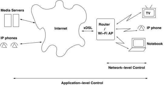
As mentioned in the Introduction, we place ourselves in a home network context, where a high–speed xDSL or cable connection is available, and a wireless router / access point (AP) provides access to it for different kinds of devices (cf Figure 1). Although in this study the actual speeds are not as relevant as the load of the network, we will use values which resemble those found in an 802.11b wi–fi network, which might include the upcoming 802.11e QoS mechanisms (see Section IV for more details). In our model, several devices such as PCs, PDAs, gaming consoles, TVs, etc. are connected to the wireless network in order to access the Internet, and to have connectivity among them. Some of these devices run ”standard” TCP or UDP applications, such as file transfers, e–mail, P2P, etc. while others run real–time applications1 (normally RTP over UDP traffic), such as VoIP, video on demand, videoconference, or multiplayer gaming. We will assume that most of these applications are working over the Internet, and therefore the bulk of the traffic will have to pass through the wi–fi AP and share the radio channel.
xDSL Internet Media Servers IP phones Notebook Network−level Control Application−level Control Router Wi−Fi AP / TV IP phone
Fig. 1. The networking context considered. We assume that network–level control can only be applied at the WLAN level (which is the only part of the network that the user may control), whereas application–level control is to be performed end–to–end.
The wireless network’s performance is very variable. Factors such as signal–to–noise ratio variations (SNR) due to external interferences, radio frequency used (2.4Ghz or 5GHz), signal fading, and multipath propagation all contribute to the degradation
of the actual network’s performance.
Variations in the SNR often imply a need to adapt to a fluctuating radio channel (Link Adaptation Mechanism) by means of more robust coding. This comes at a price, namely a drop in the effective bandwidth. The standards allow for several functioning modes, each one resulting in a smaller effective bandwidth, so globally, the available bandwidth of a wi–fi network varies in a discrete fashion among several levels. For instance, for 802.11b, there are four operation modes [4], as shown in Table I.
Mode Capacity Theoretical throughput
1 Mbps 0.93 0.93 Mbps
2 Mbps 0.86 1.72 Mbps
5.5 Mbps 0.73 4 Mbps
11 Mbps 0.63 6.38 Mbps
TABLE I
802.11B OPERATION MODES AND MAXIMAL THEORETICAL SPEEDS
When too many losses are detected, or when the SNR is too low, the network will go into the next lower–bandwidth mode. This behavior makes for violent variations in the available bandwidth, which greatly impact the performance of real–time applications. Other factors can also degrade network performance. For example, if a host detects a weak signal, it will use a low–bandwidth mode, in turn decreasing the effective bandwidth for the other hosts [5]. This happens because the contention avoidance mechanism will give all stations the same probability of access to the radio channel, and stations with a lower rate mode need more time to send the same amount of data. The transmission can also experience short loss bursts [6] due to temporary radio perturbation. These loss bursts induce delay spikes due to contention at the MAC level, which in turn may induce losses at the IP level, since the queues at the AP may overflow.
For our experiments, we used a simplified network model, like the one depicted in Figure 2. We represent the network bottleneck (the AP in this case) by means of a multiclass ./M(t)/1/H queue, in which the server service rate varies with time in a way similar to that of a wi–fi network. The server capacity hops among four different levels, the time spent on each one being an exponentially distributed random variable. After that, it either goes up (or stays at the maximum) or down (or stays at the minimum) one level. Our traffic is split in two classes, background and real–time. Our background traffic consists of file transfers (web or FTP), P2P applications, e–mail, etc., and is mostly composed of TCP traffic. This we modeled using an ON/OFF process, which allows to control the burstiness of the flows. The real–time traffic is an aggregate of audio, video, voice, game streams, etc. This kind of traffic is less bursty, so we modeled it as Poisson process. We considered that real–time traffic accounted for 50% of the packets transmitted.
λ
µ
ON/OFF
H
(t)
Fig. 2. The queuing model used. The service rate varies over time, as the available bandwidth in a wi–fi network. The buffer capacity is H, and traffic is Posson for real–time flows (we consider the aggregate of those streams), and ON/OF for background traffic.
Based on the data used in [7], we chose an average packet size of about 600B, which we used to calculate the different service rates of the AP. The queue size of the AP was set to 250 packets, and the scheduling policy used was FIFO. In order to keep the model as simple as possible, we did not represent the short loss spikes mentioned above. This should not be a problem, since at the load levels we considered, most of the losses will be due to IP–level congestion at the router/AP. In the situation considered, there are very few losses caused by delay spikes at the MAC level, compared to those caused by the bandwidth limitations of the WLAN. Figure 3 shows a bandwidth trace for a 200s period using the model described above. The available bandwidth is represented as the current service rate, in (600B) packets per second. The four service levels correspond to the four operating modes of IEEE 802.11b (as described in Table I) In Figure 4 we can see the real–time traffic loss rates (averaged every 5 seconds) for the same period and for a relatively high load case (the traffic offered had a mean of about 3.5Mbps). What was an already high loss rate during the first 120s, degrades even more when the bandwidth drops and stays low due to bad radio conditions, for instance.
Fig. 3. Example 200s bandwidth trace. The bandwidth is represented as the current service rate, in (600B) packets per second. The four service levels correspond to the four operating modes of IEEE 802.11b (as described in Table I)
0 0.2 0.4 0.6 0.8 1 0 5 10 15 20 25 30 35 40 Loss Rate Period (x5 sec)
Evolution of Average Loss Rate for Real−Time Traffic (Best Effort)
(a) 0 2 4 6 8 10 0 5 10 15 20 25 30 35 40 MLBS Period (x5 sec)
Evolution of Mean Loss Burst Size for Real−Time Traffic (Best Effort)
(b) Fig. 4. Acverage loss rates (a) and mean loss burst sizes (b) for real–time traffic over the same 200s period (note that MLBS values of 0 correspond to periods when no losses occurred).
Seeing these simulation results, it is easy to see that the QoS of this home network will not be good, and that some kind of QoS control / enforcement mechanism should be deployed. However, it is not clear just how this network behavior affects the quality of the multimedia streams as perceived by the end user. In order to be able to control this quality, it is useful be able to accurately assess it in real–time. In the next section we describe a method for doing this, along with perceived quality results for our simulation results. Note, however, that in contexts with heavy constraints, such as the one we consider, if we try to obtain the best possible quality for media streams, we might effectively shut off all the other traffic. Our goal is therefore two–fold: on the one hand we want to achieve acceptable quality levels for real–time applications, but on the other hand, we do not want penalize the other traffic more than it is necessary. The ability to assess the perceived quality of multimedia applications in real–time allows us to finely control application and network–level parameters when needed, giving more resources to media streams when they are really needed, and throttling back their consumption whenever possible.
III. ASSESSING THEPERCEIVEDQUALITY A. PSQA: Pseudo–Subjective Quality Assessment
Correctly assessing the perceived quality of a multimedia stream is not an easy task. As quality is, in this context, a very subjective concept, the best way to evaluate it is to have real people do the assessment. There exist standard methods for conducting subjective quality evaluations, such as the ITU-P.800 [8] recommendation for telephony, or the ITU-R BT.500-10 [9] for video. The main problem with subjective evaluations is that they are very expensive (in terms of both time and manpower) to carry out, which makes them hard to repeat often. And, of course, they cannot be a part of an automatic process. Given that subjective assessment is, by definition, useless for real time (and of course, automatic) evaluations, a significant research effort has been done in order to obtain similar evaluations by objective methods, i.e., algorithms and formulas that measure, in a certain way, the quality of a stream. The most commonly used objective measures for speech / audio are Signal-to-Noise Ratio (SNR), Segmental SNR (SNRseg), Perceptual Speech Quality Measure (PSQM) [10], Measuring Normalizing Blocks (MNB) [11], ITU E–model [12], Enhanced Modified Bark Spectral Distortion (EMBSD) [13], Perceptual Analysis Measurement
System (PAMS) [14] and PSQM+ [15]. For video, some examples are the ITS’ Video Quality Metric (VQM) [16], [17], EPFL’s Moving Picture Quality Metric (MPQM), Color Moving Picture Quality Metric (CMPQM) [18], [19], and Normalization Video Fidelity Metric (NVFM) [19]. As stated in the Introduction, these quality metrics often provide assessments that do not correlate well with human perception, and thus their use as a replacement of subjective tests is limited. Besides the ITU E–model, all these metrics propose different ways to compare the received sample with the original one. The E–model allows to obtain an approximation of the perceived quality as a function of several ambient, coding and network parameters, to be used for network capacity planning. However, as stated in [20] and even in its specification [12], its results do not correlate well with subjective assessments either.
The method we use [1], [2] is a hybrid between subjective and objective evaluation called Pseudo–Subjective Quality Assessment (PSQA). The idea is to have several distorted samples evaluated subjectively, and then use the results of this evaluation to teach a RNN the relation between the parameters that cause the distortion and the perceived quality. In order for it to work, we need to consider a set of P parameters (selected a priori) which may have an effect on the perceived quality. For example, we can select the codec used, the packet loss rate of the network, the end–to–end delay and / or jitter, etc. Let this set be P = {π1, . . . , πP}. Once these quality–affecting parameters are defined, it is necessary to choose a set of representative values for each πi, with minimal value πmin and maximal value πmax, according to the conditions under which we expect the system to work. Let {pi1,· · · , piHi} be this set of values, with πmin = pi1 and πmax = piHi. The number of values to choose
for each parameter depends on the size of the chosen interval, and on the desired precision. For example, if we consider the packet loss rate as one of the parameters, and if we expect its values to range mainly from 0% to 5%, we could use 0, 1, 2, 5 and perhaps also 10% as the selected values. In this context, we call configuration a set with the form γ ={v1, . . . , vP}, where vi is one of the chosen values for pi.
The total number of possible configurations (that is, the number !Pi=1Hi) is usually very large. For this reason, the next step is to select a subset of the possible configurations to be subjectively evaluated. This selection may be done randomly, but it is important to cover the points near the boundaries of the configuration space. It is also advisable not to use a uniform distribution, but to sample more points in the regions near the configurations which are most likely to happen during normal use. Once the configurations have been chosen, we need to generate a set of “distorted samples”, that is, samples resulting from the transmission of the original media over the network under the different configurations. For this, we use a testbed, or network simulator, or a combination of both.
We must now select a set of M media samples (σm), m = 1, · · · , M, for instance, M short pieces of audio (subjective testing standards advise to use sequences having an average 10 sec length). We also need a set of S configurations denoted by {γ1,· · · , γS} where γs = (vs1,· · · , vsP), vsp being the value of parameter πp in configuration γs. From each sample σi, we build a set {σi1,· · · , σiS} of samples that have encountered varied conditions when transmitted over the network. That is, sequence σis is the sequence that arrived at the receiver when the sender sent σi through the source-network system where the P chosen parameters had the values of configuration γs.
Once the distorted samples are generated, a subjective test [8], [9] is carried out on each received piece σis. After statistical processing of the answers (designed for detecting and eliminating bad observers, that is, observers whose answers are not statistically coherent with the majority), the sequence σis receives the value µis (often, this is a Mean Opinion Score, or MOS). The idea is then to associate each configuration γs with the value
µs= 1 M M " m=1 µms.
At this step, there is a quality value µsassociated to each configuration γs. We now randomly choose S1 configurations among the S available. These, together with their values, constitute the “Training Database”. The remaining S2= S − S1 configurations and their respective values constitute the “Validation Database”, reserved for further (and critical) use in the last step of the process. The next phase in the process is to train a statistical learning tool (in our case, a RNN) to learn the mapping between configurations and values as defined by the Training Database. Assume that the selected parameters have values scaled into [0,1] and the same with quality. Once the tool has “captured” the mapping, that is, once the tool has been trained, we have a function f () from [0, 1]P into [0, 1] mapping now any possible value of the (scaled) parameters into the (also scaled) quality metric. The last step is the validation phase: we compare the value given by f () at the point corresponding to each configuration γs in the Validation Database to µs; if they are close enough for all of them, the RNN is validated. If the RNN did not validate, it would be necessary to review the chosen architecture and configurations. In the studies we have conducted while developing this approach, not once did the RNN fail to be validated. In fact, the results produced by the RNN are generally closer to the MOS than that of the human subjects (that is, the error is less than the average deviation between human evaluations). As the RNN generalizes well, it suffices to train it with a small (but well chosen) part of the configuration space, and it will be able to produce good assessments for any configuration in that space. The choice of the RNN as an approximator is not arbitrary. We
have experimented with other tools, namely Artificial Neural Networks and Bayesian classifiers, and found that RNN performs better in the context considered. The ANN tend to exhibit some performance problems due to over-training, which we did not find when using RNN. As for Bayesian classifiers, we found that while they worked, it did so quite roughly, with much less precision than RNN. Besides, they are only able to provide discrete quality scores, while the RNN approach allows for a finer view of the quality function.
Let us now briefly describe the learning tool we used.
B. The Random Neural Network tool
A Random Neural Network (RNN) is actually an open queuing network with positive and negative customers. This mathematical model has been invented by Gelenbe in a series of papers, and has been applied with success in many different areas. The basics about the RNN can be found in [3], [21], [22]. The model has been extended in different directions (some examples are [23], [24], [25]). It has been successfully applied in many fields (see [26] for a survey). In particular, we can cite [27], [28], [29] for applications related to networking, or the more recent development about cognitive networks represented by papers like [30], [31], [32], [33].
Let us first explain how this model works, and how it is used as a statistical learning tool. A RNN is a stochastic dynamic system behaving as a network of interconnected nodes or neurons (the two terms are synonymous here) among which abstract units (customers) circulate. For learning applications, a feed–forward RNN architecture is commonly used. In this kind of networks, the nodes are structured into three disjoint sets: a set of “input” neuronsI having I elements, a set of “hidden” neurons H with H elements, and a set of “output” neurons O with O components. The circulating units (the “customers” of the queuing network) arrive from the environment to the input nodes, from them they go to the hidden ones, then to the output neurons and finally they leave the network. The moving between nodes is done instantaneously; this means that at any point in time, the customers in the network are in one of its nodes. With each node i in the RNN we associate a positive number µi, the neuron’s rate. Assume that at time t there are n > 0 customers at node i. We can assume that the different customers in node i are “stored” according to a FIFO schedule, although this is not relevant for the use we will make of the model. Then, at a random time T a customer will leave node i where T− t is an exponential random variable with parameter µi. More precisely, node i behaves as a ./M/1 queue. If i∈ O, the customer leaves the network. Each neuron i in sets I and H has a probability distribution associated with, denoted by (p+i,j, p−i,j)j with the following meaning: after leaving node i, the customer goes to node j as a “positive” unit with probability p+i,j or as a “negative” one with probability p−i,j. This means that#j(pi,j+ + p−i,j) = 1. If i ∈ I, p+i,j and p−i,j are zero if j∈ I ∪ O. If i ∈ H, p+
i,j and p−i,j are zero if j∈ I ∪ H. When a customer arrives at a node having n units as a positive one, it simply joins the queue (say, in FIFO order), and the number of units at the nodes increases by one. If it arrives as a negative unit, it disappears and if n > 0, one of the customers at the node (say, the last one in FIFO order) is destroyed; thus, the number of units at the neuron is decreased by one. When a negative unit arrives at an empty node it just disappears and nothing else happens. Customers arrive from outside at nodes in I according to independent Poisson flows. There is, in the general case, a Poisson stream of positive customers arriving at node i with rate λ+i and another one of negative units having parameter λ−i . The previously described network is now considered in steady state. With appropriate assumptions on its parameters (numbers λ+i and λ−i for the input neurons, rates µifor all nodes, probabilities p+i,jand p−i,jfor i∈ I and j ∈ H, and for i ∈ H and j ∈ O), the stochastic process is ergodic and there is an equilibrium regime. We are specifically interested in computing the numbers (%i)iwhere %iis the steady state probability that node i has customers (is not empty); we say equivalently that neuron i is “excited”. Assume that for any i∈ I there is some h ∈ H and some o ∈ O such that (p+i,h+ p−i,h)(p+h,o+ p−h,o) > 0. In other words, every node inI and in H can send its units outside. Then, the following result holds: assume that for all i ∈ I we have
xi= λ+i µi+ λ−i
< 1. Then assume that for all h∈ H, the number
xh= #
i∈Ixiµip+i,h µh+ #i∈Ixiµip−i,h is xh< 1. Finally, define for each o∈ O,
xo= #
h∈Hxhµhp+h,o µo+ #h∈Hxhµhp−h,o
C. Statistical learning with RNN
We want to capture the mapping between a selected set of metrics such as loss rates, bandwidths, etc. and quality. Denote by &v = v1, v2,· · · , vn the selected set of (a priori quality affecting) metrics, and by q the perceived quality of the flow.
We perform experiments providing us K pairs of values of the metrics and their corresponding quality value. Let us denote them as (&v(k), q(k))
k=1..K. We now consider a RNN with I = n input nodes, O = 1 output nodes; we set to 0 the rates of
negative units arriving from outside, and we make the following association: λ+i = vi, i = 1..n, and %o= q. Having done this, we look for the remaining set of parameters defining our RNN (the number H of hidden neurons, the rates of the neurons and the routing probabilities) such that when for all i∈ I we have λ+
i = v
(k)
i , then %o≈ q(k). To simplify the process, we first normalize the input rates (that is, the input variables v1,· · · , vn to make them all in [0, 1]), we fix H (for instance, H = 2n), and we also fix the neuron rates (for instance, mui = 1 for all i ∈ I, then µj = n for all other node). In order to find the RNN having the desired property, we define the cost function
C =1 2 K " k=1 $ %(k)o − q(k) %2 ,
where, for a given RNN, %(k)o is the probability that neuron o is excited when the input variables are λ+i = v (k)
i for all i∈ I. The problem is then to find the appropriate routing probabilities minimizing this cost function C. Doing the variable change w+i,j= µip+i,j, w−i,j= µip−i,j and denoting by &w this new set of variables (called “weights” in the area), we can write C = C( &w), the dependency on &w being through the %(k)o numbers:
%(k)o = " h∈H " i∈I (v(k) i /µi)wi,h+ µh+ " i∈I (v(k) i /µi)w−i,h w+h,o µo+ #h∈H " i∈I (v(k) i /µi)w+i,h µh+ " i∈I (v(k) i /µi)wi,h− wh,o− .
The specific minimization procedure can be chosen between those adapted to the mathematical constrained problem of minimizing C( &w) over the set:
{ &w≥ &0 : for all i &∈ O, " j
(w+
i,j+ wi,j−) = µi}.
This neural network model has some interesting mathematical properties, which allow, for example, to obtain the derivatives of the output with respect to any of the inputs, which is useful for evaluating the performance of the network under changing conditions (see next section). Besides, we have seen that a well trained RNN will be able to give reasonable results even for parameter values outside the ranges considered during training, i.e. it extrapolates well.
The method proposed produces good evaluations for a wide range variation of all the quality affecting parameters, at the cost of one subjective test.
D. Quality Assessment of the Simulation Results
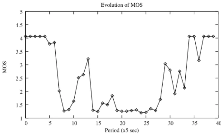
In this section we present some VoIP and video PSQA results for some traces representative of our simulation results. It can be seen that the perceived quality is quite poor in the conditions we considered. Figure 5 shows the perceived quality of a VoIP flow for the bandwidth variation pattern seen in Figure 3.
In this scale, an MOS score of 3 is considered acceptable, and the coding parameters used (codec, forward error correction, packetization interval, etc.) make for a top quality of about 4. We can see that in this case the quality is sub–par, except for relatively calm periods at the beginning and at the end of the simulation. The high loss rates observed, together with an increase in the mean loss burst size (MLBS) during those congestion periods render FEC (Forward Error Correction) almost useless in this circumstances. Although it does slightly improve the perceived quality with respect to non–protected flows, it cannot provide enough protection to achieve acceptable quality levels in this context (see below for more on FEC performance in this context). Besides the low quality scores, the quality variability with time makes for an even worse impression with the end–user. The next two figures (6 and 7) show VoIP PSQA results for different bandwidth and traffic patterns. Note that each run had a different traffic pattern, so similar bandwidths do not necessarily translate into similar MOS scores.
1 1.5 2 2.5 3 3.5 4 4.5 5 0 5 10 15 20 25 30 35 40 MOS Period (x5 sec) Evolution of MOS
Fig. 5. PSQA values for a VoIP flow and the bandwidth variation pattern seen in Figure 3 (PCM codec, no FEC, packets are 20ms long).
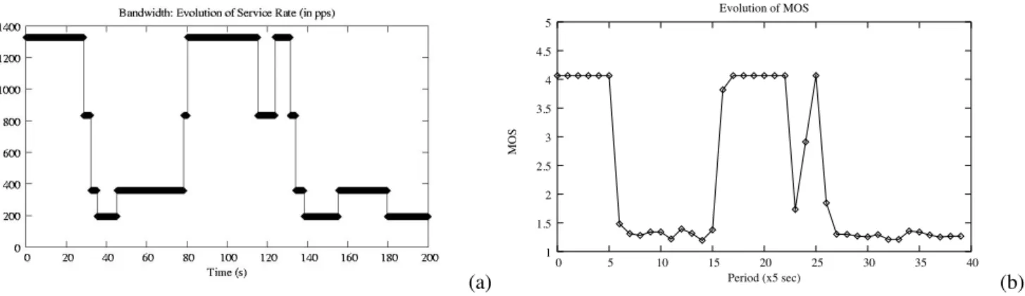
(a) 1 1.5 2 2.5 3 3.5 4 4.5 5 0 5 10 15 20 25 30 35 40 MOS Period (x5 sec) Evolution of MOS (b) Fig. 6. Second 200–second example. (a) Bandwidth and (b) MOS variation for VoIP traffic (PCM codec, no FEC, packets are 20ms long).
As in the previous case, the perceived quality is well below acceptable levels most of the time.
Figure 8 shows the bandwidth evolution and video PSQA scores for another 200–second simulation. Here we also found that the quality was poor, as expected.
It is easy to see that the congestion at the AP is generating very high loss rates and long loss bursts, which translate into bad quality scores. Loss rate traces for the second, third and fourth examples behave in a similar fashion of those for the first example (cf. Figure 4). In the next section we explore some ways to mitigate this problem and to improve the perceived quality whenever possible.
IV. IMPROVING THEPERCEIVEDQUALITY
When considering multimedia applications, there are three levels on which we can try to improve the perceived quality: • the application layer,
• the MAC layer, and • the IP layer. A. The Application Level
From an applicative point of view, there are two main problems to deal with, namely lost packets, and late packets, which in many cases count as lost (if they arrive too late to be played). In order to deal with delay and jitter, there is little to do at this level, except to use an adequate dejittering buffer, which allows to absorb the variation in delay experienced by packets, and thus mitigates undesirable effects such as clipping. For interactive applications, however, the buffer must be as small as possible, in order to minimize the end–to–end delay, which is an important quality–affecting factor. In this study we do not concern ourselves with delay issues, but concentrate instead on the impact of the loss rate and loss distribution on the perceived quality.
In order to overcome the loss of packets in the network, there are several techniques available, following the type of stream (video or audio, coding mechanism, etc.). Roughly, we can either conceal the loss (for instance by repeating the last packet in audio, or not changing the affected image region for video), or try to recover the lost data with some form of redundancy (FEC).
(a) 1 1.5 2 2.5 3 3.5 4 4.5 5 0 5 10 15 20 25 30 35 40 MOS Period (x5 sec) Evolution of MOS (b) Fig. 7. Third 200–second example. (a) Bandwidth and (b) MOS variation for VoIP traffic (PCM codec, no FEC, packets are 20ms long).
(a) (b)
Fig. 8. Fourth 200–second example. Evolution of available bandwidth (a) and MOS variation for video traffic (b).
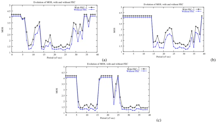
The FEC scheme described in [34], for instance, has proved itself very effective under light loss rates of up to 10 or 15% [35]. However, the violent variations in loss rate and distribution we found in our simulations require more than FEC to overcome them. Indeed, as can be seen in Figures 9 for VoIP streams, the use of FEC is not enough to obtain acceptable quality levels when the network conditions are too bad. Moreover, the addition of FEC (in particular for video streams), implies a higher load in the network. We have studied this issue for VoIP over wired networks [35], where it does not pose a real problem, since the overhead incurred is relatively small. However, in a different context such as the one we consider here, it might not be always the case. Furthermore, the addition of redundancy to video streams may imply a more significant increase in bitrate than in the VoIP case. Video FEC can need up to a 25% increase in bandwidth consumption which, given the bitrates needed for video, may imply an increase of over 1Mbps in bitrate.
For bandwidth–intensive applications such as video it may also be possible to change, if the application is able to, the coding scheme used in order to decrease bandwidth consumption in the hope of diminishing the congestion. Rate control algorithms are also available [36], which allow video streams to back down when network congestion is detected. Layered approaches [37] may also be used, which allow a host to improve video quality if it has the necessary bandwidth, or to degrade it gracefully if not. B. The MAC Level
Barring a change of the physical medium (cabling, new wireless standards, etc.), there is not much to do at the physical level. At the MAC level, however, some basic QoS provisioning mechanisms are becomign available. In [38] the authors suggest that hosts using real–time services should work in 802.11’s PCF (Point Coordination Function) mode, instead of the normally used DCF (Distributed Coordination Function). The results they present are promising, except for the fact that PCF is optional to implementers, and it is very hard to implement. As a consequence, it is not currently deployed.
However, it is interesting to point out some upcoming improvements to wi–fi networks. The 802.11e QoS extensions [6], [39] will allow to define different Access Categories in order to differentiate several service levels during the MAC contention process. It will be also possible to omit the acknowledgements and disable retransmission. In case of packets lost at the physical level, this will produce a loss at the IP level, but no extra delay will be added, which might be useful for interactive applications if the loss rate is within the bounds in which FEC is still effective. In order to better tune the 802.11e QoS parameters (e.g. set priorities among flows, set the number of retransmissions to be used, etc.), it would be very useful to understand how they (via
1 1.5 2 2.5 3 3.5 4 4.5 5 0 5 10 15 20 25 30 35 40 MOS Period (x5 sec) Evolution of MOS, with and without FEC
With FEC−1 Without FEC (a) 1 1.5 2 2.5 3 3.5 4 4.5 5 0 5 10 15 20 25 30 35 40 MOS Period (x5 sec) Evolution of MOS, with and without FEC
With FEC−1 Without FEC (b) 1 1.5 2 2.5 3 3.5 4 4.5 5 0 5 10 15 20 25 30 35 40 MOS Period (x5 sec) Evolution of MOS, with and without FEC
With FEC−1 Without FEC
(c)
Fig. 9. PSQA scores for VoIP flows, with and without FEC in a best effort context. (a) First example. (b) Second example.(c) Third example.
the performance modifications they induce at the IP level) affect the perceived quality. The use of PSQA may greatly help to this end, since it allows us to see how each network parameter affects the perceived quality. As of this writing, ongoing research is being done, aiming to assess the impact of interactivity factors such as the delay and the jitter, so that they can be also considered when performing this kind of network tuning.
C. The IP Level
At the IP level, it is possible to use a Differentiated Services architecture to give real–time streams a higher priority. This would allow to reduce both the loss rates, and the delay for the protected streams. Another possibility, if layered streams are used, is to filter the higher levels at the AP, which might help reduce the network congestion. The filtering would be done via DiffServ, e.g. marking higher levels as low–priority, or by simply dropping them with a firewall–based filter. This is actually a hybrid application / IP level approach, since it must be coordinated by both the application and the AP.
1) A Simple Proof–of–concept Example: In [40] the authors propose an AQM scheme to be used at the AP so as to improve TCP performance. In a similar spirit, but biased toward real–time streams which are basically non-responsive to congestion, we have added a very simple priority scheme to our WLAN model which allows us to see how such an architecture might affect the perceived quality. Note that we only consider the wireless link, since it is the only part of the network over which the user may have some form of control. While there exist end–to–end QoS schemes based on DiffServ, they are not widely deployed yet, nor easily adapted to micro–management such as the one we need. Furthermore, even if they were readily available, other complex issues such as pricing should be taken into account. For simplicity’s sake, we consider a simple priority scheme with few parameters needed to calibrate it.
In our model, which is loosely based on RED, the real–time traffic is always accepted if the queue is not full. For the background traffic, we define two thresholds, σ1 and σ2, with σ1 < σ2. If the number of packets in the queue is lower than σ1, the packet is accepted. If the number of queued packets is between σ1 and σ2, the packet is accepted with probability p. Finally, if the number of packets in the queue exceeds σ2, the packet is dropped. For our simulations, we used the values found in Table II. It is worth noting that this is just a first approach to a priority scheme for the WLAN, and that as such, we have not delved into issues such as optimal threshold values, or more refined backlog metrics such as those found in RED. Figures 10 through 12 show the loss rates and mean loss burst sizes (averaged every 5 seconds) for real–time flows in the three examples shown above, both for best effort and the priority scheme proposed above. It can be seen that, even though there are
Parameter Value
σ1 0.3H
σ2 0.6H
p 0.5 TABLE II
THRESHOLDS USED IN OUR SIMULATIONS. HIS THE CAPACITY OF THEAPQUEUE.
still some serious loss episodes, the situation is vastly improved.
0 0.2 0.4 0.6 0.8 1 0 5 10 15 20 25 30 35 40 Loss Rate Period (x5 sec)
Evolution of Average Loss Rate for Real−Time Traffic Best Effort Using Priorities (a) 0 2 4 6 8 10 0 5 10 15 20 25 30 35 40 MLBS Period (x5 sec)
Evolution of Mean Loss Burst Size for Real−Time Traffic (Using Priorities) Best Effort Using Priorities
(b) Fig. 10. Loss rates (a) and mean loss burst sizes (b) for real–time flows, with and without service differentiation (first example).
0 0.2 0.4 0.6 0.8 1 0 5 10 15 20 25 30 35 40 Loss Rate Period (x5 sec)
Evolution of Average Loss Rate for Real−Time Traffic Best Effort Using Priorities (a) 0 2 4 6 8 10 0 5 10 15 20 25 30 35 40 MLBS Period (x5 sec)
Evolution of Mean Loss Burst Size for Real−Time Traffic (Using Priorities) Best Effort Using Priorities
(b) Fig. 11. Loss rates (a) and mean loss burst sizes (b) for real–time flows, with and without service differentiation (second example).
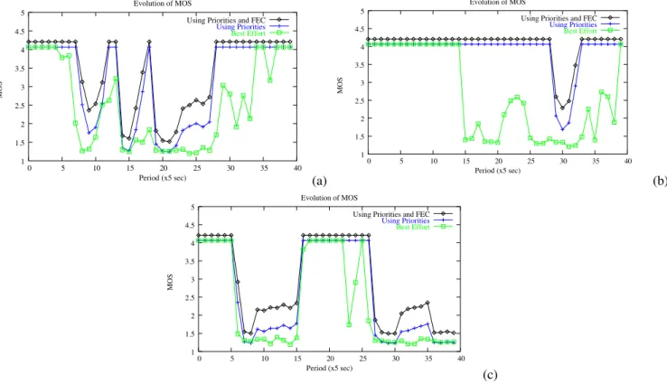
In Figure 13, we can see how the protection of multimedia flows translates into perceived quality for VoIP, while in Figure 14, we see the improvement for a video stream. It can be seen that even when using priorities, the quality does sometimes drop below acceptable levels. The addition of FEC helps to obtain better quality values, as expected. For instance, for all three cases shown in Figure 13, several periods of time where speech was barely intelligible (MOS values of about 2 points), had their quality increased to almost acceptable levels by the addition of FEC. However, the wireless network shows its limitations, since there are periods for which even the combination of FEC and priority treatment for audio packets is not enough to obtain acceptable quality levels.
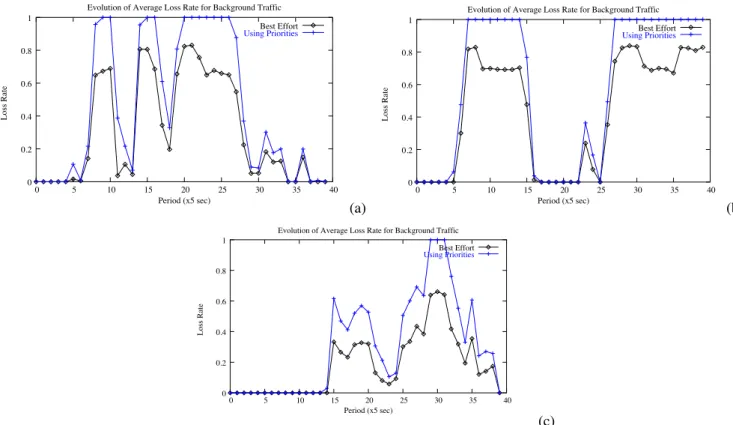
It is clear that the perceived VoIP quality is much better when the real–time packets are given a higher priority. There is, however, one problem with this approach. The improvement of real–time flows may imply a complete starvation of the background traffic, as can be seen in Figure 15.
D. Controlling the Perceived Quality
As discussed in the previous sections, it is possible to improve, at least to a certain extent, the perceived quality of multimedia applications in the networking context we defined. From application–level parameters to network QoS schemes, several tools are available that allow the user to make the best use of his network. However, blindly implementing some of all of these measures
0 0.2 0.4 0.6 0.8 1 0 5 10 15 20 25 30 35 40 Loss Rate Period (x5 sec)
Evolution of Average Loss Rate for Real−Time Traffic Best Effort Using Priorities (a) 0 2 4 6 8 10 0 5 10 15 20 25 30 35 40 MLBS Period (x5 sec)
Evolution of Mean Loss Burst Size for Real−Time Traffic (Using Priorities) Best Effort Using Priorities
(b) Fig. 12. Loss rates (a) and mean loss burst sizes (b) for real–time flows, with and without service differentiation (third example).
1 1.5 2 2.5 3 3.5 4 4.5 5 0 5 10 15 20 25 30 35 40 MOS Period (x5 sec) Evolution of MOS
Using Priorities and FEC Using Priorities Best Effort (a) 1 1.5 2 2.5 3 3.5 4 4.5 5 0 5 10 15 20 25 30 35 40 MOS Period (x5 sec) Evolution of MOS
Using Priorities and FEC Using Priorities Best Effort (b) 1 1.5 2 2.5 3 3.5 4 4.5 5 0 5 10 15 20 25 30 35 40 MOS Period (x5 sec) Evolution of MOS
Using Priorities and FEC Using Priorities
Best Effort
(c)
Fig. 13. PSQA scores for VoIP flows, for both our service differentiation scheme and best effort service. (a) First example. (b) Second example.(c) Third example. We can see the improvement due to the priority scheme used, and also to the use of FEC.
0 0.2 0.4 0.6 0.8 1 0 5 10 15 20 25 30 35 40 Loss Rate Period (x5 sec)
Evolution of Average Loss Rate for Background Traffic Best Effort Using Priorities (a) 0 0.2 0.4 0.6 0.8 1 0 5 10 15 20 25 30 35 40 Loss Rate Period (x5 sec)
Evolution of Average Loss Rate for Background Traffic Best Effort Using Priorities (b) 0 0.2 0.4 0.6 0.8 1 0 5 10 15 20 25 30 35 40 Loss Rate Period (x5 sec)
Evolution of Average Loss Rate for Background Traffic Best Effort Using Priorities
(c)
Fig. 15. Loss rates for background traffic, with and without service differentiation. (a) First example. (b) Second example. (c) Third example.
is not enough. The DiffServ–like mechanisms should only be used when needed, so as not to punish other applications if it’s not necessary.
Being able to accurately assess the perceived quality in real time with tools such as PSQA, it is possible to react to network impairments as they happen, without sacrificing other applications’ performance unless really needed. Among the options available to perform QoS control in the context we described, there are:
• Access control – It is possible to prevent certain flows from being created if the network conditions are not appropriate,
e.g. if the predicted PSQA scores are too low. The user might then manually choose to shut down other applications which are less important to him, such as P2P software, for instance. This could be also done automatically via a centralized server, in which low–priority applications would be identified to be throttled back if necessary.
• Application–level adjustments – From changing the FEC offset to changing the codec used, many parameters are easily
adjustable at the application level. Even if by themselves these changes may not be enough, they certainly help, and they might even help reduce congestion.
• IP–level filtering – If multi–layer streams are being used, the AP could filter the upper layers in order to avoid congestion. The perceived quality would then degrade gracefully, and in conjunction with other measures (such as ECN for competing TCP flows) the loss spikes can be avoided or at least reduced.
• DiffServ schemes – As we have previously seen, this kind of approach can greatly improve the perceived quality even when
the network conditions are very bad. It would be interesting to use the quality feedback obtained by means of PSQA to fine–tune the parameters of these mechanisms, and to mark packets only when necessary, so as not to punish the background traffic if not needed. This should be also used in conjunction with the QoS provisions of 802.11e, if available, so as to allow marked flows a prioritary access to the medium.
V. CONCLUSIONS
In this paper we have studied the quality of multimedia (voice and video) streams in a likely future home networking context. We have studied the performance of the wireless link, and how it affects the perceived quality of real–time streams. To this end we have used PSQA, a real–time quality assessment technique we have previously developed and validated. This technique allows to measure, in real time and with high accuracy, the quality of a multimedia (or audio, or video) communication over a
packet network. This means that (for the first time, as far as we know), we have a tool that allows an automatic quantitative evaluation of the perceived quality giving values close to those that would be obtained from real human users (something that can be obtained otherwise only by using a panel of observers). PSQA is based in Random Neural Networks. This paper can be seen as an application of PSQA to the performance analysis of some important aspects of home networks and illustrates a success of IA techniques in networking.
Our results show that the wireless technologies that are currently most widely deployed are not ready for the kind of use outlined in our context, and that QoS control mechanisms should be used if acceptable quality levels are to be achieved.
We have proposed a simple proof-of-concept priority management scheme at the IP level, and studied how such a scheme would affect the perceived quality. The results obtained, while not perfect, show a marked improvement over best effort service, at the price of occasionally starving the background traffic. We have not delved into optimizing the queuing parameters for the priority model we used yet, but this is a subject of further research. Again, the key element is the availability of a technique for the assessment of quality as perceived by the user, accurately, automatically and efficiently so that it can be used in real time.
Finally, we have suggested several ways in which the QoS of multimedia streams could be improved in the context considered, in real–time, and based on their quality as perceived by the end–user.
Further work in this area will include an in-depth study of the control options for the 802.11e QoS mechanisms, and how to implement them to improve the quality of media streams. As of this writing, we are starting to work on an NS–2 based model, which should allow us to have a better idea of how these mechanisms affect QoS. Another point on which we are currently working is the study of interactivity factors for conversational quality. This includes the impact of delay and jitter on the perceived quality, as well as other factors such as the interactivity level of the conversation itself (measured, for instance, as proposed in [41]), and their integration into PSQA.
REFERENCES
[1] S. Mohamed and G. Rubino, “A Study of Real–time Packet Video Quality Using Random Neural Networks,” IEEE Transactions On Circuits and Systems
for Video Technology, vol. 12, no. 12, pp. 1071 –1083, Dec. 2002.
[2] M. S., G. Rubino, and M. Varela, “Performance evaluation of real-time speech through a packet network: a Random Neural Networks-based approach,”
Performance Evaluation, vol. 57, no. 2, pp. 141–162, 2004.
[3] E. Gelenbe, “Random Neural Networks with Negative and Positive Signals and Product Form Solution,” Neural Computation, vol. 1, no. 4, pp. 502–511, 1989.
[4] P. M¨ulhethaler, WiFi 802.11 et les r´eseaux sans fil. Eyrolles, 2002.
[5] M. Heusse, F. Rousseau, and A. Duda, “Performance Anomaly of 802.11b,” in Infocom’03, Mar. 2003.
[6] R. Rollet and C. Mangin, “IEEE 802.11a, 802.11e and Hiperlan/2 Goodput Performance Comparison in Real Radio Conditions,” in GlobeCom’03, 2003. [7] J. Incera and G. Rubino, “Bit-level and packet-level, or Pollaczec-Khintine formulae revisited,” in QEST’04, 2004.
[8] ITU-T Recommendation P.800, “Methods for Subjective Determination of Transmission Quality.” [Online]. Available: http://www.itu.int/
[9] ITU-R Recommendation BT.500-10, “Methodology for the subjective assessment of the quality of television pictures,” in International Telecommunication
Union, Mar. 2000. [Online]. Available: http://www.itu.int/
[10] J. Beerends and J. Stemerdink, “A Perceptual Speech Quality Measure Based on a Psychoacoustic Sound Representation,” Journal of Audio Eng. Soc., vol. 42, pp. 115–123, Dec. 1994.
[11] S. Voran, “Estimation of Perceived Speech Quality Using Measuring Normalizing Blocks,” in IEEE Workshop on Speech Coding For Telecommunications
Proceeding, Pocono Manor, PA, USA, Sept. 1997, pp. 83–84.
[12] ITU-T Recommendation G.107, “The E-model, a Computational Model for Use in Transmission Planning.” [Online]. Available: http://www.itu.int/ [13] W. Yang, “Enhanced Modified Bark Spectral Distortion (EMBSD): an Objective Speech Quality Measrure Based on Audible Distortion and Cognition
Model,” Ph.D. dissertation, Temple University Graduate Board, May 1999.
[14] A. Rix, “Advances in Objective Quality Assessment of Speech over Analogue and Packet-based Networks,” in the IEEE Data Compression Colloquium, London, UK, Nov. 1999.
[15] J. Beerends, “Improvement of the P.861 Perceptual Speech Quality Measure,” ITU-T SG12 COM-34E, Dec. 1997. [Online]. Available: http://www.itu.int/ [16] W. Ashmawi, R. Guerin, S. Wolf, and M. Pinson, “On the Impact of Policing and Rate Guarantees in Diff-Serv Networks: A Video Streaming Application
Perspective,” Proceedings of ACM SIGCOMM’2001, pp. 83–95, 2001. [Online]. Available: citeseer.nj.nec.com/ashmawi01impact.html
[17] S. Voran, “The Development Of Objective Video Quality Measures That Emulate Human Perception,” in IEEE GLOBECOM, 1991, pp. 1776–1781. [18] C. van den Branden Lambrecht, “Color moving picture quality metric,” in Proceedings of the IEEE International Conference on Image Processing, Sept.
1996. [Online]. Available: citeseer.nj.nec.com/vandenbrandenlambrec96color.html
[19] ——, “Perceptual Models and Architectures for Video Coding Applications,” Ph.D. dissertation, EPFL, Lausanne, Swiss, 1996.
[20] T. A. Hall, “Objective Speech Quality Measures for Internet Telephony,” in Voice over IP (VoIP) Technology, Proceedings of SPIE, vol. 4522, Denver, CO, USA, Aug. 2001, pp. 128–136.
[21] E. Gelenbe, “Learning in the Recurrent Random Neural Network,” Neural Computation, vol. 5, no. 1, pp. 154–511, 1993.
[22] ——, “Stability of the Random Neural Network Model,” in Proc. of Neural Computation Workshop, Berlin, West Germany, Feb. 1990, pp. 56–68. [23] ——, “G-Networks: new Queueing Models with Additional Control Capabilities,” in Proceedings of the 1995 ACM SIGMETRICS joint international
conference on Measurement and modeling of computer systems, Ottawa, Ontario, Canada, 1995, pp. 58–59.
[24] E. Gelenbe and J. Fourneau, “Random neural networks with multiple classes of signals,” Neural Computation, vol. 11, no. 3, pp. 953–963, 1999. [25] E. Gelenbe and K. Hussain, “Learning in the multiple class random neural network,” IEEE Trans. on Neural Networks, vol. 13, no. 6, pp. 1257–1267, 2002. [26] H. Bakircioglu and T. Kocak, “Survey of Random Neural Network Applications,” European Journal of Operational Research, vol. 126, no. 2, pp. 319–330,
2000.
[27] E. Gelenbe, C. Cramer, M. Sungur, and P. Gelenbe, “Traffic and video quality in adaptive neural compression,” Multimedia Systems, vol. 4, no. 6, pp. 357–369, 1996.
[28] C. Cramer, E. Gelenbe, and H. Bakircioglu, “Low bit rate video compression with Neural Networks and temporal sub-sampling,” Proceedings of the IEEE, vol. 84, no. 10, pp. 1529–1543, 1996.
[29] C. Cramer and E. Gelenbe, “Video quality and traffic QoS in learning-based sub-sampled and receiver-interpolated video sequences,” IEEE Journal on
Selected Areas in Communications, vol. 18, no. 2, pp. 150–167, 2000.
[30] E. Gelenbe, R. Lent, and Z. Xu, “Design and performance of cognitive packet networks,” Performance Evaluation, vol. 46, pp. 155–176, 2001. [31] E. Gelenbe, “Towards networks with cognitive packets,” in Proc. IEEE MASCOTS Conference, San Francisco, CA, 2000, pp. 3–12.
[32] ——, “Reliable networks with cognitive packets,” in International Symposium on Design of Reliable Communication Networks, Budapest, Hungary, Oct. 2001, pp. 28–35, invited Keynote Paper.
[33] ——, “Cognitive Packet Networks: QoS and Performance,” in Proc. IEEE Computer Society MASCOTS02 Symposium, Fort Worth, TX, Oct. 2002, pp. 3–12, opening Keynote.
[34] J.-C. Bolot, S. Fosse-Parisis, and D. F. Towsley, “Adaptive FEC-based error control for Internet telephony,” in Proceedings of INFOCOM ’99, 1999, pp. 1453–1460. [Online]. Available: citeseer.nj.nec.com/bolot99adaptive.html
[35] G. Rubino and M. Varela, “Evaluating the Utility of Media–dependent FEC in VoIP Flows,” in QofIS’04, Barcelona, Spain, Sept. 2004.
[36] R. Rejaie, M. Handley, and D. Estrin, “Quality adaptation for congestion controlled video playback over the Internet,” in SIGCOMM ’99: Proceedings of
the conference on Applications, technologies, architectures, and protocols for computer communication. ACM Press, 1999, pp. 189–200. [37] ——, “Layered Quality Adaptation for Internet Video Streaming,” 2000. [Online]. Available: citeseer.ist.psu.edu/rejaie00layered.html
[38] B. Crow, I. Widjaja, J. G. Kim, and P. Sakai, “Investigation of the IEEE 802.11 Medium Access Control (MAC) Sublayer Functions,” in INFOCOM
’97: Proceedings of the INFOCOM ’97. Sixteenth Annual Joint Conference of the IEEE Computer and Communications Societies. Driving the Information Revolution. IEEE Computer Society, 1997, p. 126.
[39] IEEE 802.11 Working Group, “Draft Amendment to Standard for Information Technology Telecommunications and Information Exchange between Systems LAN/MAN Specific Requirements Part 11 Wireless Medium Access Control (MAC) and Physical Layer (PHY) Specifications: Amendment 7: Medium Access Control (MAC) Quality of Service (QoS) Enhancements,” 2004.
[40] S. Yi, M. Keppes, S. Garg, X. Deng, G. Kesidis, and G. Das, “Proxy-RED: An AQM Scheme for Wireless Local Area Networks,” in IEEE ICCCN’04, 2004.
[41] F. Hammer and P. Reichl, “Hot discussions and Frosty Dialogues: Towards a Temperature Metric for Conversational Interactivity,” in 8th International