HAL Id: hal-00967044
https://hal.archives-ouvertes.fr/hal-00967044
Submitted on 27 Mar 2014HAL is a multi-disciplinary open access
archive for the deposit and dissemination of sci-entific research documents, whether they are pub-lished or not. The documents may come from teaching and research institutions in France or abroad, or from public or private research centers.
L’archive ouverte pluridisciplinaire HAL, est destinée au dépôt et à la diffusion de documents scientifiques de niveau recherche, publiés ou non, émanant des établissements d’enseignement et de recherche français ou étrangers, des laboratoires publics ou privés.
Probabilistic Relational Models for Customer Preference
Modelling and Recommendation
Rajani Chulyadyo, Philippe Leray
To cite this version:
Rajani Chulyadyo, Philippe Leray. Probabilistic Relational Models for Customer Preference Modelling and Recommendation. [Research Report] Laboratoire d’Informatique de Nantes Atlantique. 2013. �hal-00967044�
A Technical Report
on
Probabilistic Relational Models for Customer Preference
Modelling and Recommendation
Rajani Chulyadyo, Philippe Leray
Abstract:
Nowadays, recommender systems are implemented in many domains to assist users in discovering interesting items/products from large amount of online information. While traditional recommendation approaches mainly deal with single dyadic relationships be-tween users and items, data in real world are generally conceptualized in terms of ob-jects and relations between them. Probabilistic Relational Models (PRMs) [9] intend to fill this gap by learning probabilistic models from relational data. In this report, we present an adapted version of a unified recommendation framework originally pro-posed by Huang et al. [15] that uses the concept of PRM and builds a Na¨ıve Bayesian classifier to make recommendations. We mainly aim at using this model in coldstart situation where users/items are new to the system or the system itself is new. We apply the framework on MovieLens data and show that the model is actually capable of making recommendations to new users though the model is too simple to provide good recommendations to old users.
R´esum´e :
De nos jours, les syst`emes de recommandation sont utilis´es dans de nombreux domaines avec pour objectif d’aider les utilisateurs `a d´ecouvrir des produits/items int´eressants parmi un volume important d’informations en ligne. Alors que les approches de recom-mandation traditionnelles traitent le cas de relations simples entre utilisateurs et items, les donn´ees r´eelles sont g´en´eralement conceptualis´ees en terme d’objets et de relations entre objets. Les mod`eles relationnels probabilistes (PRM) [9] ont pour but de faire la passerelle en proposant des mod`eles probabilistes `a partir de donn´ees relationnelles. Dans ce travail, nous pr´esentons une adaptation du cadre de recommandation “unifi´e” propos´e initialement par Huang et al. [15] qui utilise le concept des PRM et construit un classifieur de Bayes na¨ıf pour effectuer la recommandation. Nous nous proposons d’utiliser ce mod`ele dans un contexte de “d´emarrage `a froid” o`u les utilisateurs ou les items sont nouveaux dans le syst`eme, ou mˆeme lorsque le syst`eme se construit. Nous appliquons cela aux donn´ees MovieLens et montrons que ce mod`ele est capable de faire de bonnes recommandations `a des nouveaux utilisateurs, mˆeme s’il est trop simple pour la recommandation `a des utilisateurs existants.
Contents
1 Introduction 1
2 State of the art 1
2.1 Recommender systems . . . 1
2.1.1 Collaborative filtering . . . 2
2.1.2 Challenges in collaborative filtering . . . 2
2.2 Bayesian networks . . . 3
2.2.1 Inference in Bayesian networks . . . 4
2.2.2 Learning Bayesian networks . . . 4
2.3 Probabilistic Relational Model . . . 5
2.3.1 Inference in PRM . . . 7
2.3.2 Learning PRM . . . 7
3 PRM for recommender systems: review and comparative study 8 3.1 Reviews . . . 8
3.2 Discussion . . . 11
4 Our approach 12 4.1 The framework . . . 12
4.1.1 Relational attributes generation . . . 13
4.1.2 Markov blanket detection . . . 15
4.1.3 Model creation . . . 15 4.1.4 Recommendation . . . 15 4.2 Challenges addressed . . . 16 4.2.1 Data sparsity . . . 16 4.2.2 Coldstart problem . . . 16 4.2.3 Scalability . . . 17 5 Experimental evaluation 17 5.1 Implementation . . . 17 5.2 Dataset . . . 18 5.2.1 Dataset preparation . . . 18
5.3 Evaluation procedure and performance metrics . . . 19
6 Results 20
7 Future work 20
1
Introduction
With the advancement of information technologies, huge amount of online information are being available day by day. Need for systems to filter useful and interesting information from the overwhelming collection of information has led to different information retrieval (IR) technologies. Recommender system (RS) is one of such IR tools that helps users discover items or products of their interest. Nowadays, we can find such systems in many websites that we visit frequently, for e.g. YouTube, Facebook, IMDb, Amazon etc. Recommender systems have been successfully implemented in many domains such as music/video/movie recommendations, social networking, e-commerce, online newspapers/blogs, hotel/flight reservation etc. Many algorithms have been developed and proposed for effective recommendation. Most of these ap-proaches rely on flat data representation such as user-item matrix to predict relation between target users and items. However, most real-world systems are generally composed of repetitive patterns and are conceptualized in terms of objects and relations between those objects. To apply traditional recommender algorithms, the relational data needs to be converted to flat representation which is not a good idea as it may introduce statistical skew and lose useful information that might help us understand the data. Moreover, in the domains where recommender systems are often used (for e.g. e-commerce), users and items grow continuously. Recommender systems need to be scalable to keep up with the growing size of the dataset without degrading the performance.
The motivation for this work is the need for scalable recommendation algorithms that can learn from relational data and also make prediction even when there is not enough data. Recently, there has been growing interest in Probabilistic Relational Model (PRM) [9] which aims at learning probabilistic model from relation data. A PRM models the uncertainty over the attributes of objects in the domain and the uncertainty over the relations between the objects [7]. As a recommendation problem involves the relations between customers and products, we apply this relational learning framework to learn and predict item preference for a given customer. This is a collaborative effort of two PhD students and three DMKM students to develop a framework to work with PRMs programmatically and use the framework to implement a recommender system as an application of PRM. We review some approaches to build recommender systems using PRMs and select one promising approach for implementation. The selected approach [15] is characterized by the capability of unifying different recommendation techniques such as content-based, demographics-based and collaborative filtering techniques into a single framework with the use of PRMs and Bayesian Networks only. It is also capable of creating new relational attributes relevant for recommendation through the use of slot chains introducing the notion of multi-set operator, and uses of a classifier built around the Markov Blanket attributes for recommendation. I focused on the implementation of the multi-set operators and recommendation framework with Na¨ıve Bayes classifier. I also participated in the implementation of framework for evaluating recommender systems. Besides, we also performed some experiments to check how this framework can handle cold-start problem.
The remainder of the report is organized as follows. Section 2 provides an overview of recommender systems, Bayesian networks and PRMs. We present a comparative review of five different approaches for recommendation using PRMs in section 3. Then, we present our adaptation to one of the reviewed approaches in section 4. Section 5 describes our implementation and evaluation method and the exper-imental results are presented in section 6. Finally, in section 7, we discuss about the possible areas of enhancement and conclude the report in 8.
2
State of the art
2.1 Recommender systems
Recommender Systems (RSs) are systems that discover the items that a user can find interesting from a (usually large) collection of items and suggest them to the users. Nowadays, we can find such systems in many websites that we visit frequently, for e.g. YouTube, Facebook, IMDb, Amazon etc. Recommender systems have been successfully implemented in many domains such as music/video/movie recommenda-tions, social networking, e-commerce, online newspapers/blogs, hotel/flight reservation etc. Given the users or user models and the items, RSs compute relevance score that gives how relevant an item could be
to a user. User models can be users’ ratings, preferences, demographics or situational context etc. while items can be anything depending on the domain, for e.g. music, movies, books, news, cities, restaurants, friends, products etc. Basically, data that a recommender system uses to make recommendations involve three entities – items to suggest, users who made some kind of interactions with the items and who will receive recommendations and transactions which refer to the interactions, for e.g. users’ rating, buying action etc., made by the users on items. One way to visualize this data is as a matrix (table) where each row represents a user, each column represents an item and each cell represents the transaction between the user with the item, empty cells denote no transaction between the user and the item. We call this a User-Item matrix. Recommender techniques are categorized into four classes based on the data they take [16] – Content-based, Collaborative Filtering, Demographics-based and Hybrid approaches.
Content-based filtering takes the items’ features only into consideration to make recommendations. It considers past behavior of the users but not the community whereas collaborative filtering (CF) uses preferences of the community without considering the items’ features. For example, content-based filtering recommends movies that are similar to the ones the user liked in the past while collaborative filtering approach recommends movies that are popular in the user’s community. Demographics-based filtering uses users’ demographic information such as age, gender, occupation etc. to find interesting items. Hybrid approach is a combination of the previous classes of recommendation techniques. Here we will focus on recommendation using collaborative filtering as we are more interested in it on this project though the RS we are implementing is a hybrid one.
2.1.1 Collaborative filtering
The basic assumption behind collaborative filtering is that similar users show similar behaviours (or preferences) and this correlation of customer preferences can be exploited to predict future preferences of customers. As an example, if a user A like some movies that B also likes (or rates similarity), then it is likely that A would like other movies liked by B. This approach only uses transaction data to identify users with similar preferences (neighbours in other word) and make recommendations based on the neighbours’ preferences. Collaborative filtering is considered to be the most popular technique in RS and a wide range of CF algorithms are available. Su and Khoshgoftaar [25] have categorized CF algorithms into three classes – Memory-based, Model-based and Hybrid CF algorithms.
Memory-based CF algorithms use the complete set of data to make recommendations. These al-gorithms iterate through the entire transaction list to discover the neighbours of the target user and predict items that may interest the user. On the other hand, model-based approach deals with the rec-ommendation problem by first building a model from the observed data and then using this model to make predictions. The models incorporate factors that help the system predict users’ future interactions. Hybrid CF algorithms combine different CF techniques to build systems that perform better than the individual techniques.
2.1.2 Challenges in collaborative filtering
Major challenges a CF system faces are scalability and data sparsity issues. Ricci et al. [21] and Su and Khoshgoftaar [25] have listed other challenges of CF techniques. However, we will address only these two major challenges in this project.
CF techniques are often implemented in large e-commerce websites where the systems aim at selling as much products as possible and the more customers they can attract, the more revenue they will generate. Such systems need to keep up with the continuously growing users and items. Traditional CF algorithms, especially memory-based, are generally not scalable as they require large computational resources for large datasets. Some techniques like dimensionality reduction, model-based CF etc. have emerged to address scalability issue.
Another issue a CF algorithm needs to take into consideration is the possibility of data sparsity. Recommender systems are mostly applicable in the scenario where the users cannot filter interesting items themselves from overwhelming collection of items. In such situation, user-item matrix will be very sparse as users can rate only a small subset of the collection of items. This may significantly degrade the
Figure 1: An example of Bayesian Network [20]
performance of the CF algorithms. A typical situation of data sparsity challenge is cold start problem when the system cannot recommend to a new user who has not rated any items yet or when the system cannot recommend a new item to users since it is not rated by anyone. Demographics-based CF handles this issue to some extent. However, it may be a show-stopper where users rate only the items recommended to them or there is no means other than CF to discover new interesting items.
2.2 Bayesian networks
Probabilistic Graphical Models (PGMs) represent joint probability distributions through graphs and parameters and compactly encode a complex distribution over a high-dimensional space. In Probabilistic Graphical Models, the nodes represent the random variables in the domain and the edges represent the direct probabilistic relation between these variables. This graph specifies the product form of the distribution. Bayesian Network is one of the common classes of PGM which uses a directed acyclic graph and represents joint probability distribution as a product of conditional probabilities. Another class of PGM is Markov Network which uses an undirected graph and represents joint probability distribution as a product of potentials. Here, we will be discussing about Bayesian Networks only.
A Bayesian Network [20] consists of two components: a directed acyclic graph (DAG) and a set of conditional probability distributions (CPDs). The nodes in the graph correspond to random variables X1, X2, . . . Xn each of which has a finite set of mutually exclusive states. A Bayesian network associates with each variable Xi a conditional probability P (Xi|P ai), where P ai ∈ X is the set of variables that are called the parents of X. In the graph, edges direct to a random variable Xi from its parents. The CPD of the random variables without any parent will be their prior distribution. Bayesian Networks achieve compact representation of probability distribution by exploiting conditional independence properties of random variables. Every node in a Bayesian network is conditionally independent of its non-descendants given its parent. This conditional independence assumption enables Bayesian networks to simplify the joint probability distribution given by the Chain rule as follows:
P(X1, X2, . . . Xn) = Y
i
P(Xi|P ai) (1)
Figure 1 shows an example of a Bayesian Network adapted from [20]. All the random variables in this example take binary states: Yes or No. Every node is associated with a CPD. The edges in the graph show the probabilistic dependences of the variables. Earthquake can make alarm go off. If there is an earthquake, it’s likely that there will be an announcement on radio. There are edges from Earthquake
to Alarm and Radio Announcement as they are directly dependent. However, Earthquake is not directly dependent on Burglary, i.e. observing earthquake does not change the chances of getting burglary in a house. Thus, there is no edge between these variables. However, if we observe Alarm, these variables become conditionally dependent.
2.2.1 Inference in Bayesian networks
Inference in Bayesian networks generally refers to: finding the probability of a variable being in a certain state, given that other variables are set to certain values; or finding the values of a given set of variables that best explains (in the sense of the highest MAP probability) why a set of other variables are set to certain values [6]. In small BNs, exact inference can be performed where we analytically compute the conditional probability distribution over the variables of interest. The most common exact inference methods are Variable Elimination method, Message passing algorithm for trees or polytrees[20] and Junction tree algorithm [17]. Since exact inference in an arbitrary Bayesian Network for discrete variables is NP-hard [5], approximate inference is performed in large, complex BNs. Approximate inference involves heuristic and stochastic techniques which are not guaranteed to give the correct answer for a given query, but often return values that are close to the true values [22]. Markov Chain Monte Carlo (MCMC) method, Belief propagation for general graphs [19] are some of the common approximate inference methods. 2.2.2 Learning Bayesian networks
One way to build a Bayesian network is to collect expert knowledge and create the model based on it. However, this is not feasible all the time as it may be difficult to find experts in the domain of the interest. Besides, the data in the hand may not always be in accordance with experts’ opinion. When the data keeps on changing, the data may show different behaviors at different time and hence the model will need to be updated with the changing data. Many algorithms have been developed in order to learn Bayesian networks from the observed data. Learning a Bayesian network involves two tasks: (a) learning parameters (i.e. conditional probabilities), and (b) learning structure (i.e. DAG).
Parameter learning
Various statistical and Bayesian methods are available for learning conditional probabilities in BNs from different kinds of data. Maximum likelihood estimation (MLE) is a usual statistical approach to learn parameters of BNs given the structure and complete data. It estimates the parameters that maximize the probability of getting the data given the parameters, i.e. P (D|θ). The maximum likelihood estimate for a given CPT has a nice property that the maximum likelihood parameters are simply the frequency counts for a given value and its parents’ values in the data. MLE is often complex when there are unob-served variables. Expectation Maximization with MLE is commonly used in such scenario. Maximum a Posteriori (MAP) and Expectation a Posteriori (EAP) are some Bayesian approach to parameter learning. Structure learning
Learning Bayesian network structures is NP-hard [4]. Even for 10 nodes, there are 4.2 × 10¹⁸
possible DAGs. So, exhaustive search to find the exact structure is impossible. Various techniques have been developed to learn BN structure. Daly et al. [6] have broadly classified them into three approaches – score and search approach, constraint-based approach and dynamic programming approach. In score-based methods, a BN is viewed as a probabilistic model that must best fit the data while in constraint-based approach, a BN is seen as an independence model and its structure is learnt by testing conditional independence between the variables. Score and search approach looks for the DAG space in order to maximize a scoring/fitness function that assigns a score to a state in the search space to see how good a match is made with the sample data. Bayesian Dirichlet (BD) criterion, Bayesian information criterion (BIC), Akaike information criterion (AIC), minimum description length (MDL) and minimum message length (MML) are some examples of scoring functions. Greedy search is commonly used heuristic search method. It starts with a model with no links between the nodes and iteratively adds, reverts or deletes
Figure 2: An example of a relational schema
links in the current DAG scoring the resulting DAG at each step. There are many other hybrid methods which combine local search with global learning procedure. These methods typically search one local neighbourhood for each node and learn global structure using this local information. Neighbourhood can be parents and children of a given node or its Markov blanket attributes which refer to parents, children and spouses of a given node. Min-max Hill-climbing algorithm [27] is an example of hybrid structure learning method that uses MMPC [1] for local information along with greedy search for global structure search.
2.3 Probabilistic Relational Model
Bayesian networks have been one of the main models for reasoning under uncertainty. The simplicity of their specification is one of the reasons of their success. However, one of the difficulties in Bayesian networks is to create and maintain the model of very large domains. Large and complex systems are generally composed of repetitive patterns and can be conceptualized in terms of objects and relations between those objects. Bayesian networks are not sufficient to model this construct as they lack the concept of objects and their relations. They are designed for modeling attribute-based domains, where we have a single table of independent and identically distributed (IID) instances [11]. They require a propositional data set whereas real word data are often stored and managed using relational represen-tation. Converting relational data into flat data representation for statistical learning may introduce statistical skew and lose useful information that might help us understand the data. Thus, in order to learn statistical model such as Bayesian Network, Probabilistic Relational Models (PRMs) were emerged which specify probability model for classes of objects rather than simple attributes. A PRM models the uncertainty over the attributes of objects in the domain and the uncertainty over the relations between the objects [7]. It basically defines a template for probabilistic dependencies in typed relational domains which can be later instantiated with a particular set of objects and relations between them.
A Probabilistic Relation Model is comprised of two components: a relational schema of the domain and a probabilistic graphical model describing the probabilistic dependencies between the attributes of the classes in the domain. We follow here the notations and symbols from [9].
Relational schema
Relational schema describes a set of classes X and the relation between them. Each class X ∈ X is described by a set of descriptive attributes A(X) and a set of reference slots R(X) which is a way to allow objects to refer to another objects. In the context of a relational database, a class refers to a single database table, descriptive attributes refer to the standard attribute of tables, for e.g. age, gender, education of users, type/price of products etc. and reference slots are equivalent to foreign keys.
An attribute X.A of a class X ∈ (X ) takes values on a range V(X.A). A reference slot of a class X that relates an object of class X to an object of class Y is denoted as X.ρ where Domain[ρ] = X and Range[ρ] = Y . While a reference slot gives a direct reference of an object with another, objects of one class can be related to objects of another class indirectly through other objects. Such relations are represented by Slot chain which is a set of reference slot or inverse slot with the range of a slot being the domain of the next slot. Formally, a slot chain is a set of slots ρ1, ρ2, . . . ρn such that for all i, Range[ρi] = Domain[ρi+1].
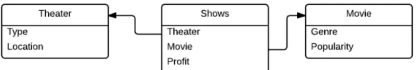
An example of a relational schema is depicted in the figure 2 which shows relations between classes X = {Movie, Shows, Theater}. The class Shows has a descriptive attribute Shows.Profit and two reference slots R = {Shows.Theater, Shows.Movie}. The value space of Movie.Genre could be V(Movie.Genre) =
Figure 3: An example of a PRM taken from [9]
{Action, Thriller, Comedy} Domain of the reference slot Shows.Theater is Shows and range is Theater. This reference slot relates the objects of class Shows with the objects of class Theater. Alternatively, this relation can be viewed in the opposite direction, i.e. objects of Theater are related to objects of Shows. This reverse way of viewing a relation is defined by an inverse slot ρ−1 which is interpreted as the inverse function of ρ. Thus, in this example, the inverse slot of Shows.Theater would be Shows.Theater−1 such that Domain[Shows.Theater−1] = Theater and Range[Shows.Theater−1] = Shows. An example of a slot chain would be [Shows.Theater ].[Shows.Theater]−1.[Shows.Movie] which could be interpreted as all the movies shown in the particular theater.
Probabilistic model
A relational schema is instantiated with a set of objects for each class, the values of the attributes and the relations between the objects. The probability distribution of such an instance I of a relational schema is specified by a probabilistic model in a PRM. The model consists of a dependency structure and the parameters associated with it. Dependency structure is a result of parent-child relations of attributes just like in Bayesian networks. The dependencies can be between the attributes of the class or between the attributes of the different classes. The associated parameters are conditional probability distributions of each node given its parents.
Another important concept in PRM is the notion of Aggregator. The previous example is not a very good example to explain this notion. So, an example taken from [9] is depicted in the figure 3. Aggregators come into play when there is dependency between the objects that have one-to-many or many-to-many relations. In the example, Student.Ranking depends probabilistically on Registration.Grade. As a student can register in more than one course, Student.Ranking will depend on Registration.Grade of more than one Registrationobject and this number will not be the same for all students. So, in order to get a summary of such dependencies, aggregators are introduced. An aggregator, denoted γ, is a function which takes a multi-set of values and produces a single value as a summary of the input values. Average, mode, cardinality etc. can be used as an aggregation function. In the example, γ(Student.Registration.Grade) is a parent of Student.Ranking.
Formally, a Probabilistic Relational Model (PRM) Π for a relational schema R is defined as follows [9]. For each class X ∈ X and each descriptive attribute A ∈ A(X), we have:
• a set of parents Pa(X.A) = U1, . . . Ul, where each Ui has the form X.B or γ(X.τ.B), where τ is a slot chain and γ is an aggregator of X.τ.B.
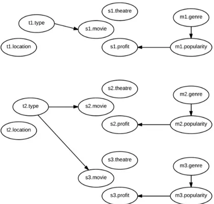
Figure 4: An example of a simple PRM with all conditional probabilities
Figure 4 is an example of a simple PRM that corresponds to the relational schema in the figure 2. All dependencies and associated parameters are shown here. The dashed lines between the classes indicate that the objects of these classes are related through slot chains.
2.3.1 Inference in PRM
Inference is performed on a Ground Bayesian Network (GBN) obtained from a PRM for the given instance I. A GBN is generated by a process (also called unrolling) of copying the associated PRM for every object in I. Thus a GBN will have a node for every attribute of every object in I and probabilistic dependencies and CPDs as in the PRM. Figure 5 shows a GBN associated with the PRM in figure 4 for an instance with the following objects:
• 2 Theaters : t1 (?, Center), t2 (?, Outside) (Theater.Type unknown / determined by PRM) • 3 Shows : s1 (t1, m1, Low), s2 (t2, m2, High), s3(t2, m3, Low)
• 3 Movies : m1 (Foreign,?), m2 (Thriller, ?), m3(Thriller, ?) (Movie.Popularity unknown / deter-mined by PRM)
Standard inference algorithms for Bayesian network can be used to query the GBN. Exact inference can be performed in small GBNs. Regularities in GBNs make it possible to apply exact inference algorithms. However, GBNs can be very large and complex. In such cases, exact inference will not be impossible and hence, approximate inference methods such as Markov Chain Monte Carlo (MCMC) method, Belief propagation for general graphs [19] etc. will need to be applied to query the GBN.
2.3.2 Learning PRM
As with Bayesian networks, learning PRM involves two tasks – learning parameters and learning structure. Learning parameters
Given a dependency structure S and an instance I, the task in parameter estimation is to learn a parameter set θS that defines the CPD for this structure. For a PRM, the likelihood of a parameter set θS is: L(θS|I, σ, S) = P (I, S, θS). Parameter estimation is performed using standard statistical or Bayesian method. Sufficient statistics are computed in MLE over I using queries for relational data (for e.g. SQL queries in relational database).
Figure 5: An example of a Ground Bayesian Network Learning structure
PRM structure learning is inspired from classical methods of learning standard BN structures. Getoor used score and search approach to learn PRM structure. Unlike in BNs, there is a constraint in assigning edges between nodes in PRM. The edges must be between two attributes from either the same class or the classes reachable through reference slots. Standard scoring functions can be used to score the structures. Friedman et al. [7] proposed walking through the slot chains to discover potential parents for each attribute and applying the search procedure on this set of parents. In order to avoid infinite space of relational attributes, the algorithm proceeds in multiple phases keeping the length of slot chain fixed at each phase. The search for potential parents and the corresponding structure begins with the slot chains of length 0 which is increased by 1 at each phase until a predefined slot chain length limit is reached or there is no improvement in the PRM structure.
3
PRM for recommender systems: review and comparative study
As a part of this project, five different approaches to build recommender systems using PRMs were studied and compared with each other to find the best one to implement. The studied approaches are explained under the title of the corresponding page in the following section.
3.1 Reviews
Collaborative Filtering Using PRMs
Getoor and Sahami [10] have presented an approach to build a recommender system using Probabilistic Relational Models. Their approach is based on the models proposed by Ungar and Foster [28], Hofmann and Puzicha [14] which use Bayesian Networks for collaborative filtering. The main idea in these models is to cluster the users and the items separately and make prediction based on the clusters instead of working on a large set of user-item matrix which makes the recommender system scalable. Clustering is performed based on the history of users (or items) and their neighbourhood. Ungar and Foster [28] propose repeated clustering technique to find clusters of users and items in which firstly, users are clustered based on the
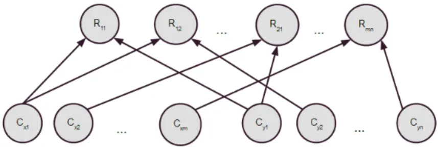
Figure 6: A Bayesian Network for two-sided clustering
items they like (or purchase) and items based on the users who like them and in the subsequent phases, users are clustered based on the item clusters and items based on movie clusters. In these models, we have latent variables Cxi for each user xi and Cyi for each user yi such that Cxi ∈ {Cx1, Cx2, . . . Cxm}
and Cyi ∈ {Cy1, Cy2, . . . Cym} where users and items are clustered into m and n clusters respectively.
For each user-item pair, the existence of relation rij between user i and item j depends on their clusters. The model is depicted in the figure 6.
In this model, strong assumptions are made that each person (also each item) belongs to only one cluster and that every relation rijmust have the same local probability model. These assumptions make it possible to represent this model compactly by PRMs. In PRM, every user and item are assigned to a class and these classes determine the relation between the user and the item. With the use of PRM, dependencies of other attributes of the entities can also be included in the model. For example, age, gender, profession etc. of users can determine their classes or vice versa and there could be dependencies between these attributes themselves or even with the attributes of item. This enables PRMs to make better predictions since the effect of many variables can be seen from a single model. This also enables PRM to handle cold start problem. If a user has not liked / purchased any items yet, PRMs can still make recommendation for him based on the attributes of this user. However, the system would be no more doing collaborative filtering but it will be more like a demographic filtering system or some hybrid system.
A Unified Recommendation Framework Based on PRMs
Huang et al. [15] developed a hybrid approach capable of combining different recommendation techniques. The framework is based on PRMs and can gather different kinds of information useful for recommendation from relational data. For example, users’ demographics, items’ characteristics, ratings made by users’ neighbours etc. can be collected from a relational schema using this approach. The authors have employed the fundamental idea of learning PRM structure by walking through the slot chains to find optimal dependency structure of the PRM. They use the same concept to capture information that can be valuable for recommendation. They have illustrated that long slot chains can capture interesting patterns and the use of such long slot chains along with aggregation and multiset operations can enhance the performance of recommender systems. They limit the length of slot chain in heuristic structure search algorithm [7] to create a finite attribute space from which attributes that can be relevant for recommendation are filtered out as Markov blanket attributes of the target attribute. They perform constrained model search to identify optimal dependency structure surrounding the target attribute. From this optimal dependency structure, a Na¨ıve Bayes classifier is then built around the Markov Blanket attributes. The basic workflow for this method is as follows: first, relational attributes are generated by walking through the slot chains, then Markov Blanket attributes are detected for the target attribute (for e.g. rating attribute of Rating class) and a Na¨ıve Bayesian classifier is built from the Markov Blanket such that all Markov blanket attributes are independent of each other given the target attribute. The classifier is then used to recommend items.
(a) (b)
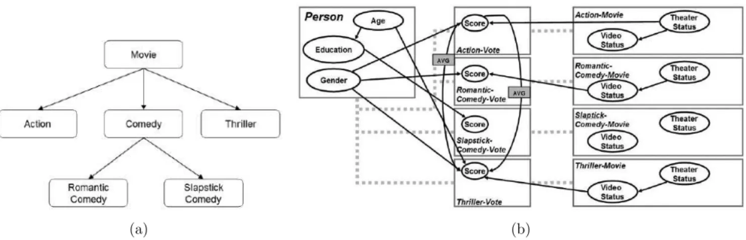
Figure 7: (a) Hierarchy of Movie class and (b) hPRM proposed by Newton and Greiner Hierarchical Probabilistic Relational Models
In a context of movie-rating dataset, a user’s rating on some movies may depend on his rating on some other movies which is a way to make recommendation to users based on their movie ratings. As rating depends on itself, this information cannot be expressed in a PRM because it requires the class-level dependency structure to be a DAG to ensure that the instance-level ground Bayesian network generated from the PRM also is a DAG. In order to address this issue, Newton and Greiner [18] proposed Hierarchical Probabilistic Relational Model (hPRM). In this approach, the item class is divided hierarchically into different classes and an hPRM is built using the leaves of the hierarchy. Now, rating of one type of movie can depend on rating of different type of movie which is not possible in standard PRM. The hierarchy and the hPRM proposed by Newton and Greiner [18] are shown in figure 7.
To learn the hierarchy, greedy partitioning approach is proposed here. hPRM is learnt in the same way as a standard PRM. Inference is performed on the unrolled hPRM.
A RBN-based Recommender System Architecture
Ben Ishak et al. [2] proposed another hybrid approach for recommendation based on Relational Bayesian Network (RBN). They tried to find the solution to the same problem that Newton and Greiner had addressed, i.e. the scenario where users’ ratings depend on the previous ratings of the users’ neighbours. As a solution to this, they propose to make a copy of the Rating class such that the original Rating class called Sound-votes represents the observed votes/ratings and the duplicate class called Forecast-votes represents objects that we suppose their presence. Now, the ratings from Forecast-votes can depend on the ratings from Sound-votes without creating a cycle in the original class dependency structure. The advantage of this approach is that it limits structure search procedure and generates a simple model. However, this obtained model is not a strong model for recommendation. Hence, the model is enriched by providing an appropriate model instantiation to each active user based on a set of rules derived from recommendation requirements. This approach is capable of addressing data sparsity, cold start and scalability problems and can also provide different recommendation techniques from the same model. Combining User Grade-based Collaborative Filtering and PRMs (UGCF-PRM)
Gao et al. [8] proposed a hybrid method for recommendation that combines collaborative filtering and PRMs. They introduced the concept of a user grade function which is based on the user-item matrix and is an increasing function with the number of rating items. The user-grade for the users with large number of rating items will be higher than that for the users with few ratings. Thus, user-grade function acts like an adaptive weight for different grade users when combining the prediction from collaborative filtering with that from PRM. Let Gu be the user-grade function for the target user u, PuiN BS and PuiP RM be the prediction from neighbour-based CF and that from PRM respectively for the target item i. The combined prediction Pui is then given as the weighted average of the two predictions.
Pui= Gu· PuiN BS+ (1 − Gu)· PuiP RM (2) It is clear from equation 2 that as the user grade function increases, UGCF-PRM is dominated by CF. Thus, only when the target user has few ratings, the prediction from PRM will be dominant.
3.2 Discussion
Getoor and Sahami [10]’s work builds a hybrid recommender system rather than a collaborative one as explained in the paper. The good points of this model are that it is easier to interpret than a Bayesian network, is extensible and can handle cold start and scalability problems. However, the paper does not explain how to learn such PRM and how to make actual recommendations from such model. Besides, the effectiveness of the model mainly depends on the quality of clusters and it is difficult to obtain good clusters that can assign items/users to only one cluster. Also, the authors have not presented experimental results. Hence, we do not have a clear vision of how effective the model could be. Moreover, the specification of PRM used in this paper is different from the current specification which is better than the previous one.
The introduction of mutli-set operation has increased the expressiveness of the recommendation frame-work proposed by Huang et al. [15]. It allows to capture data patterns that cannot be captured by simple (short) slot chains of regular PRMs. The framework unifies different recommendation techniques si-multaneously. The authors have illustrated the unification of content-based, demographics-based and collaborative filtering techniques which resulted in a good recommendation performance. However, the difficulty with this approach is that the relational feature space can grow very large based on the length of the slot chain and feature construction and model estimation process can go computationally inten-sive. However, we found this approach of recommendation promising as it uses the concepts of PRM and BN only to combine different methods of recommendation. Besides being scalable, it can also address sparsity and cold start problem better which is not mentioned in the literature but we aim at verifying this through our experiments.
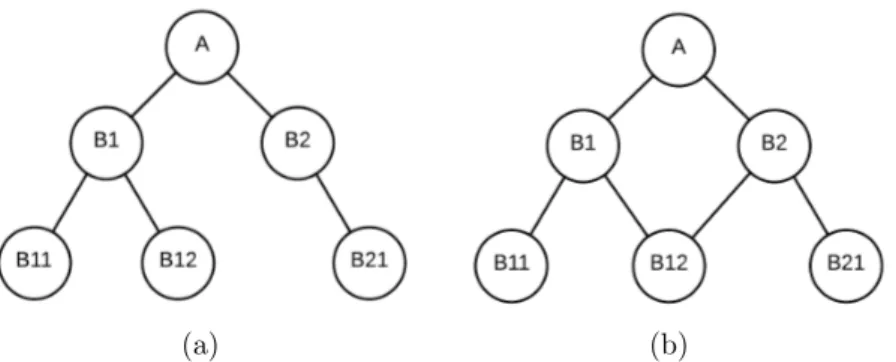
Though the result presented by Newton and Greiner [18] shows that hPRMs perform better than standard PRMs and some other algorithms, there are some limitations with this approach. First, though the same notations and examples from Getoor’s PRM with Class Hierarchy (PRM-CH) [9] have been used, hPRM is different from PRM-CH and it does not actually use the hierarchical structure of PRM. Only leaves are taken to make subclasses. This is like dividing a class into different subclasses and learning PRM as a regular PRM. Thus, the inner classes are always missed out. For example, hPRM cannot address the hierarchy as shown in the figure 8 where class B2 can be an interesting class but since it has one child, it is never considered while making the hPRM. Because of the same issue, it cannot address lattice structure which is very common in real world. For example, a movie can have more than one genre. Movie subclasses cannot always be disjoint as opposed to what was proposed by the authors. Second, the greedy partitioning used to create the hierarchy is not a good approach since the partitions created using this approach depend on the dataset used.
UGCF-PRM approach aims to overcome simultaneously the most common problems of CF: sparsity, scalability and cold start. The use of PRM in this model is basically to handle cold start problem. It does not actually exploit the capability of PRM in recommendation. For the target user with many ratings, the effect of PRM becomes negligible. Besides, the authors give an example PRM but do not say anything about learning it. In the sample PRM, the target attribute depends on attributes of all other classes with some intra-class dependencies. However, to achieve such model, we need either expert knowledge or some probabilistic computation which is not mentioned by the authors. So, we cannot fully rely on the result obtained from the PRM. In fact, the whole model can be achieved from Huang et al.’s approach which does not use traditional CF algorithms, instead makes use of Na¨ıve Bayesian classifier for simplification of the problem.
After reviewing these approaches to build recommender systems, we found that Huang et al.’s unified framework is the most promising. Unification of different recommendation techniques and the recom-mendation process is all done by the use of PRMs and BNs only without the need to combine with other
(a) (b)
Figure 8: Sample hierarchies hPRMs cannot address: (a) a hierarchy where a node has only one (leaf) child, (b) a lattice structure where a node can be a subclass of more than one class
frameworks. Besides, we liked the concept of multi-set operation which enhances the expressiveness of PRM. Though the framework is computationally intensive, it has shown good performance and it seems the framework can be extended to improve its capability. Therefore, we are implementing it not only to see the performance but also to prove it is capable of addressing major challenges of recommender system algorithms, i.e. cold start problem, data sparsity and scalability.
4
Our approach
We are adapting the approach proposed by Huang et al. [15] in our implementation. In this section, we will describe our approach to implement a recommender system using this recommendation technique in detail and will also explain how it addresses recommendation problems.
4.1 The framework
The framework proposed by Huang et al. aims at dealing with binary transaction data rather than rating data. Customers’ purchase history is an example of binary transaction data where the recommendation problem is to predict the existence of a customer-product pair. So, a new attribute Exists is introduced in the relational data to indicate whether the pair exists. All the records in purchase history will have Exists= 1 and for the customer-product pairs that are not in the purchase history take Exists = 0. The objective is to create a classifier with Exists attribute as a target attribute and predict the probability of the existence of the customer-product pair given other attributes. The framework we are implementing is little different than this. Instead of binary transaction data, we are focusing on rating data. The reason behind this is twofold: first, rating data is commonly used by traditional techniques in many recommender systems, so we can compare the performance of our recommendation approach with different other approach. Moreover, MovieLens1
, a popular dataset for evaluating recommendation technique, that we are using to evaluate our system also has rating data. Second, binary transaction data approach may not be applicable in all scenarios. As an instance we can consider an application where users can like items and the Like table has information about who liked the items. If the collection of items is huge, only a small subset of items will be liked by users. Binary transaction data approach may interpret the non-existence of user-item pair as “items that are not liked by users”. This affects the recommendation of items which are not liked by any users yet.
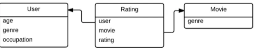
The process will be explained in detail in the following section. From now onwards, we will refer to the relational schema of MovieLens dataset (figure 9) for any examples as our implementation is tested in this dataset.
1
Figure 9: A relational schema for MovieLens dataset
4.1.1 Relational attributes generation
The first task in this recommendation approach is to find all possible attributes that can be derived from slot chains. Slot chains give how an object is related to other objects through reference (or inverse reference) slots. We generate relational attributes by traversing through slot chains. For example, Rat-ing.user represents the user who did the particular rating; [Rating.movie].genre represents the genre of the movie of the given rating. Similarly, [Rating.movie−1].[Rating.movie].[Rating.user ] represents the users who rated the target movie. Longer slot chains can create interesting attributes which can be relevant for recommendation purpose. For example, [Rating.movie−1].[Rating.user ].[Rating.user−1].[Rating.movie] gives all the movies liked by the users who like the particular movie.
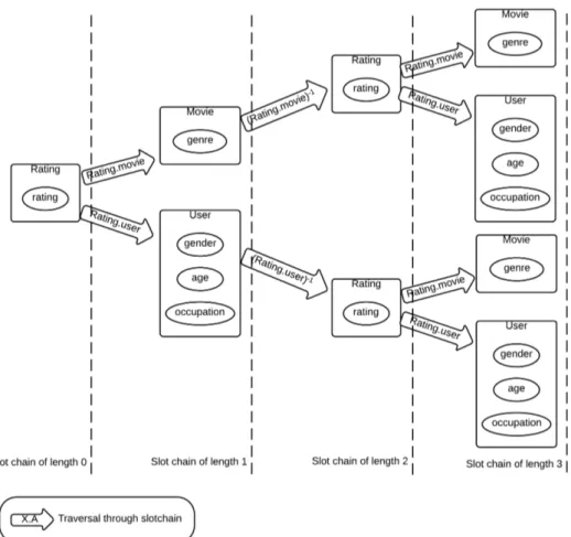
Traversing through slot chains can go to infinity if we do not put a constraint on the search. We limit the length of slot chains so as to restrict the search space. Corresponding to figure 9, figure 10 shows the possible paths for traversing through slot chains for slot chain length of upto 3. Here, if we start traversing from Rating class, we obtain a relational attribute Rating.rating for slot chain of length 0. For slot chain length = 1, we get [Rating.user ].age, [Rating.user ].gender, [Rating.user ].occupation and [Rating.movie].genre as new relational attributes. If we end up at the Movie in slot chain of length 1, then the only way to get a slot chain of length 2 is to traverse back to Rating through the inverse slot chain [Rating.movie−1], thus we will get [Rating.movie].[Rating.movie−1]. The interpretation of this slot chain would be “all the ratings for the target movie”. We can generate other attributes similarly. Multi-set operators
Referring to figure 10, the slot chain [Rating.movie] gives a single movie for the particular rating. But when we go back to Rating from Movie through inverse slot chain, we may get multiple ratings for the particular movie. In such case, we need aggregation functions to summarize the multiset. Huang et al. extended Friedman et al. [7]’s idea of deriving new relational attributes by combining multisets obtained from two individual slot chains before aggregating them. This is, in fact, a good idea as it can increase the expressiveness of the attributes. For example, [Rating.movie].[Rating.movie−1].[Rating.user ] represents the set of users who rated the target movie and [Rating.user ].[Rating.user−1].[Rating.movie].[Rating.movie−1]. Rating.user ] gives the set of users who have rated at least one movie rated by the target user. Intersection of these two multi-valued attributes will give a set of users who rated the target item as well as at least one movie that the target user has rated. Thus, the attribute derived by intersecting these two attributes contain more information relevant for recommendation. An example of intersection is illustrated in figure 11.
Huang et al. have defined a Multi-set operator as follows:
A multi-set operator φkon k multi-valued attributes A1, . . . , Akthat share the same range V(A1) denotes a function from V (A1)k to V (A1).
The multiset operation that the authors have suggested are union and intersection. However, other set operations such as difference may also result in a good model. After applying a multiset operator, the resulting multiset are aggregated to include them in the probabilistic dependency structure of PRM. As all possible combinations of individual slot chains that share the same range need to be ex-plored in order to derive new attributes with mutliset operation and aggregation, it is possible to obtain duplicate attributes that give the same information about the relation between the same enti-ties. For example, intersection[Rating.user].[Rating.user−1].[Rating.movie]. [Rating.movie−1].[Rating.user],
Figure 10: Slot chain traversal
[Rating.movie].[Rating.movie−1].[Rating.user] represents the path between target user and target item which can be expressed as U –M′–U′–M where U and M are target user and movie respectively, U′and M′ are other users and movies respectively and relation between users and movies (i.e. Rating) is expressed by –. Similarly, intersection[Rating.movie].[Rating.movie−1].[Rating.user].[Rating.user−1].[Rating.movie], [Rating.user].[Rating.user−1].[Rating.movie] also represents the path between target user and target item expressed as M –U′
–M′
–U . Both of these expressions represent the same path between target user and target item (with the same number of hop). In order to detect such duplicates, the authors have presented a method where slot chain path σ(τ1, τ2) is constructed before performing intersection of two applicable derived attributes such that duplicate attributes will have the same slot chain path (σ) or its reverse (σ−1).
A slot chain path σ(τ1, τ2) for a multiset intersection between two derived attributes is given by
σ(τ1, τ2) = τ1.τ2−1
Let τ1 = ρ11.ρ12. . . . ρ1m and τ2 = ρ21.ρ22. . . . ρ2n such that Range[τ1] = Range[τ2]. Then, σ(τ1, τ2) = τ1.τ2−1= ρ11.ρ12. . . . ρ1m.ρ−12n. . . . .ρ
−1 22.ρ
−1 21
Before performing intersection operation, slot chain path is constructed and if σ or σ−1 correspond to existing attributes, intersection will not be performed to avoid duplicates.
4.1.2 Markov blanket detection
The idea behind the generation of relational attributes is to identify the attributes within Markov Blan-ket of the target attribute so as to avoid searching for the complete model describing all probabilistic dependencies. Markov Blanket refers to the set of children, parents and spouses of a node in a Bayesian Network. In our example, we want to predict the target attribute Rating.rating, so we find the Markov blanket attributes of this attribute. In order to detect Markov blanket, the authors use a naive method to identify the optimal partial dependency structure surrounding the target attribute. However, we are using IAMB (Incremental Association Markov Blanket) algorithm [26] in our implementation as we think that IAMB is a state-of-the-art solution for this task. In this algorithm, a heuristic function is used to measure the association between two variables given the estimated Markov Blanket variable. We are using Mutual Information as the association measure.
4.1.3 Model creation
Once the Markov blanket of the target attribute has been detected, we build a model using these at-tributes. One way to build a model is to search for possible dependency structure among these atat-tributes. We can use some heuristic search approach to find the exact structure of the attributes. However for simplicity, we follow the authors and build a Na¨ıve Bayesian classifier and predict P r(V |X) where V is the target attribute (Rating.rating in our example) and X are the Markov Blanket attributes. Like PRMs, the parameters of this model are learned using Maximum Likelihood. However, experts’ opinion can be taken when there is no enough data to learn a good model. More on this scenario will be in explained in the following section. A Na¨ıve Bayes classifier with three Markov blanket attributes is shown in figure 12.
4.1.4 Recommendation
Recommendation is performed on the complete Na¨ıve Bayesian classifier. Two approaches to do recom-mendation have been identified:
Figure 12: A simple classifier for recommendation Approach I
An approach for recommending movies/items is to first find the combination of values that the Markov blanket attributes would take that maximize the probability that the target attribute will have high rating and then find the items that match this combination. The problem associated with this approach is the complexity of the query (SQL query if relational database is used) to get the items that match the best combination of the attribute values.
Approach II
A naive way to discover movies that a user might like is by finding for each movie m the probability that the user will like m and picking the ones with high probability values. For instance, if users’ liking is determined by the rating they give to movies, we compute the probability of getting high rating for the movies and recommend the movies that have the maximum probability values of getting high rating. This approach is simple and intuitive. However, it is not efficient when there is a large collection of movies/items. Currently, we are working on this approach as our dataset is not very big.
4.2 Challenges addressed
The ability to perform demographic-based, collaborative and content-based filtering from the same ap-proach has made this recommendation technique address major challenges that recommendation systems face. Based on the data in hand, it can generate models that support different recommendation technique. For instance, when there is enough (rating) data, it can generate a model that supports collaborative filtering. In the absence of rating data (or when not enough rating data is available), attributes for content-based or demographic-based filtering will come into play. Because of the versatility of this ap-proach, it can handle the following three major recommendation issues.
4.2.1 Data sparsity
A user-item matrix is not needed to learn this type of recommender systems. Since the model is learnt directly from relational data, data sparsity is not a problem for this model.
4.2.2 Coldstart problem
Coldstart problem occurs when the system does not have enough data to make recommendations to users. Traditional approaches which rely on users’ rating cannot provide recommendation to new users who have not made any ratings yet. In order to solve this issue, demographics based filtering technique emerged which uses demographic information to predicting interesting items. Content-based approaches where features of items to be recommended are used to make predictions also address this issue. However, we can think of another scenario where these approaches cannot make prediction, that is when the system is completely new and there is no ratings at all (or very few number of ratings). In such scenario, it is
difficult to learn users’ behavior based on their demographics (the same for content-based approach). In the following, we will discuss how both of these situations can be handled by our approach.
Case I: New user/item in an old system
In this case, there will already be enough rating data from which users’ behavior based on their demo-graphics or users’ preferences over items based on item features can be learnt. Thus, a content-based or demographic-based or hybrid recommender system can be achieved in this situation which will enable the system to address coldstart problem. A model can be built from attributes with short slot chains (for e.g. slot chains of length 1) to obtain such a system.
Case II: New user/item in a completely new system
In a completely new system, there will be no (or few) rating data. Learning a model without data is impossible. So, in such case, a model can be built from experts’ knowledge. In such case, Markov blan-ket detection and model parameter learning will not be performed. Instead, probabilistic dependencies between various relational attributes can be suggested by experts. Here also, the relational attributes will be generated by short slot chains to obtain demographic-based or content-based or hybrid solution since longer slot chains which produce collaborative filtering results are not of any use in this situation. Such a model will be capable to make some prediction. Though the performance may not be good or as expected, such models can be used to engage users and collect rating data. Once a good number of ratings have been collected, the model can be refined to get a better model.
4.2.3 Scalability
This recommender system is a model-based system where a Bayesian network model is generated from the observed data and recommendation is made by inferencing in the model. It does not need to scan through all the ratings to make prediction for every user. The difficult part of this system is the construction of the model. Once the model is ready, it can be used to perform recommendation without altering the model even when the data grows. However, to ensure good performance of the model, it needs to be evaluated from the observed data in some time interval. As long as the evaluation result is satisfactory, the model does not need to be updated.
5
Experimental evaluation
We are developing a prototype of recommender system. The first version of the system has been imple-mented and experiments are performed to evaluate the impleimple-mented recommender system. This section will discuss about the implementation of the system and its evaluation.
5.1 Implementation
The recommender system prototype is developed in C++. It is built on the top of PILGRIM API which contains core framework for PRM and structure learning. The library ProBT2
has been used to construct a Na¨ıve Bayesian classifier and perform inference from it. Boost3
library has been used to work with the graphs. The first version of the system is capable of constructing a classifier with relation attributes generated from slot chains of length 1 only. In our case, longer slot chains require aggregator functions which are still in development phase. For a proof of concept, we evaluate the system with an evaluation framework that is being developed as a part of this recommender system. Currently, it is in its initial phase and can compute some basic metrics only.
2
http://www.probayes.com/index.php/en/products/sdk/probt
3
Figure 13: Relational schema of Kyzia dataset
5.2 Dataset
We have two kinds of dataset – one with good number of rating data and the other one with items and users only which can be used for testing cold-start problem (Case II in the previous section). The first dataset we are using is MovieLens dataset which is a well-known dataset for recommendation, and the second one is a set of users and properties from Kyzia4 website. The relational schema of MovieLens dataset is already presented in figure 9. The interesting part of the second dataset is that it is from a new system, so we do not have information about interaction between users and properties. The interaction can be modeled into users’ purchase preference that will make it a binary transaction data or into users’ rating which will make it a rating data. Since the system we are implementing works with rating data, we prefer the latter option. However, as explained in section 4.2.2, the recommendation model for this kind of data needs experts’ advice. Evaluation of such model needs live user experiments since we do not have data to perform offline evaluation [13]. We present the relational schema of this dataset here (figure 13) but keep the evaluation for future.
5.2.1 Dataset preparation
Our system deals with discrete random variables only. So, we need to discretize all continuous variables. In some cases when a discrete random variable takes a large number of states, we need to convert the states into some compact states to reduce the number. For example, ‘age’ of a user can take integer values from 0 to some defined number, let’s say 120. But if we keep all states of age, we will have 121 states. We can reduce the number of such states by defining some ranges of age, for e.g. 0 5, 6 10, 11 -20 etc. MovieLens data already comes with such range. So, we do not require discretizing any variables. But for Kyzia data, we took experts’ advice to discretize continuous variables.
Since we are not considering hierarchy of classes, we include in our MovieLens subset dataset only those movies that belong to a single genre. For proof of concept, we are working on a small subset of
4
MovieLens data. We have created two subsets of the original dataset. The first dataset contains the ratings of the first 100 users for the movies with single genre. So, we have 100 users, 2025 movies and 3546 ratings in this dataset. We also have a dataset to test cold start problem. This dataset contains some users who are not present in the previous datasets to simulate new users in the system. Another approach for creating datasets can be the approach of Sarwar et al. [23] who only consider users who have rated twenty or more movies.
5.3 Evaluation procedure and performance metrics
In order to evaluate our system, we divided our dataset into train and test sets. We construct a Na¨ıve Bayesian classifier from the train dataset and test it on the test dataset. One problem in this approach is that the trained model may not represent the actual observation since the train and the test sets may have dependent data and hence the probability distributions in the trained model may not represent the actual distribution. So, we need to take care of the size of train and test sets while partitioning the data. We followed Huang et al. [16] and Sarwar et al. [23] and partitioned the dataset into 80% train and 20% test sets. The partitioning was done based on the rating data. Around 80% of the rating data was randomly assigned to the train dataset and the remaining ratings were placed into the test set. Then the corresponding users were fetched into both sets. However, we kept all the movies into both sets. To simulate coldstart situation, we created a dataset containing some users who are not in the train set. This dataset is then used in testing to evaluate the system under coldstart. Table 1 shows the size of the datasets.
A better approach to evaluate the system is to apply leave-one-out method where all but one rating is used to create the classifier and the one not used in the training is used to evaluate the system. In this case, the trained model better represents the observed distributions but the evaluation is computationally intensive as it needs to do it for all the ratings. Since we have more than 3000 ratings, this method is not virtually possible. Another evaluation approach is to apply n-fold cross validation as suggested by [18] where the dataset is split into n partitions and (n − 1) partitions are used in training the model keeping the remaining one partition for testing. Training and testing are done n times so that all the partitions are used once for testing. Though this method can produce good evaluation result, it can be computationally intensive too since we need to repeat the evaluation task n times. Thus, we are applying our 80%-20% train and test sets as this approach is also followed for evaluating recommender systems using MovieLens data by many other researchers [16, 23, 12].
Table 1: Summary of datasets
Dataset # Users # Movies # Ratings
Train 91 2025 2846
Test 51 2025 700
Test set for coldstart problem 10 2025 201
Top-N recommendations method is applied to evaluate the system. In this method, movies are ranked on the basis of the probability of getting high ratings (“4” and “5” are considered to be high ratings in our experiments) from the target user and the top-N movies are then recommended to the user. The recommended quality is then measured by comparing the recommended movies with the user’s actual preferences. The following metrics [24, 13] are computed to measure performance of the system.
Precision(P ) = Number of hits
N (3a)
Recall(R) = Number of hits
Number of high rated movies in the test set (3b) F-measure(F ) = 2 × P × R
where hits is the number of actual preferences that appear in the top-N recommendations.
The above metrics are computed for each user and the average over all users is taken as the overall metric of the algorithm.
6
Results
Because of the dependencies in the development of the project, some parts of the system could not be completed by the time of this writing. The major components that are yet being implemented are Markov blanket detection and cardinality aggregator. Since Markov blanket detection algorithm was not available, we tested our system with some manually chosen variables only. Due to the complexity of queries for long slot chains as well as the uncompleted aggregator, we could evaluate the system with relational attributes with slot chain of length 1 only.
We evaluated the implemented recommender system by applying top-10 and top-20 recommendations on two models over two test sets – one for general testing and one for testing under coldstart. The first model consists of three attributes: User.gender, User.age and Movie.genre whereas the second one consists of four attributes: User.gender, User.age, User.occupation and Movie.genre with Rating.rating being the parent of all in both models. Table 2 shows the performance measures of different models. Both models seemed to perform better when top 20 movies were recommended. These tested models are basically a hybrid one that is a combination of demographic-based and item-based techniques. Such systems are particularly useful in coldstart scenario.
Here, F-measure values for general test set are slightly better than those for coldstart test set. This suggests that performance of these models in coldstart situation is comparable with that when the user is not new. The magnitude of the metrics is also in similar range as compared to that of the results obtained by [16] though our datasets are completely different. However, the metrics values are smaller than those of the results from Sarwar et al. [23] approach. One of the reasons for this must be the simplicity of the models. The models we have built are very basic ones. They consider very short slot chains only and do not have collaborative filtering concept yet. Another reason might be the datasets used for testing. Though the authors used MovieLens dataset, we are not using the same subset and they are considering only users who have rated 20 or more movies which is not the case in our dataset. Another reason for low metrics values must be an issue of evaluation approach. Since we are recommending only N movies, movies after N + 1 ranks are skipped even when they have the same probability of getting high ratings as movies at rank N . This can be a reason of getting low recall. Besides, we are lacking the result of Markov blanket detection algorithm. So, the results are based on our hypothetical models which can be different from the actual ones.
7
Future work
In the previous section, we have presented the results of evaluation of our approach for building a recommender system. The results show that the system is capable of making recommendations even when the user is new and has no rating at all. We have not seen the actual capability of the system yet because we still need to implement the system with long slot chains and integrate it with multiset operators. The first thing we need to finish in order to come up with a complete recommender system is the implementation of Markov blanket detection algorithm and cardinality aggregator. We expect to get better models after the integration of this algorithm. Another important aspect for improvement is the optimization of the system. The current system is not as fast as it is expected to be. It can be improved by using better technique to do inference and by optimizing the code.
Though we have got some results as a proof of concept, it is difficult to judge a system by evaluating on a single dataset with few performance measures. Evaluation on multiple datasets and implementation of more performance metrics such as Rank score [3], RMSE (Root Mean Square Error) can make it more clear about the quality of the recommendations made by the system. Besides, we have not considered the movies that belong to more than one genre. One area of improvement can be addressing such hierarchical information.
Table 2: Performance measures of recommender systems
Test set Attributes N = 10 N = 20
Precision Recall F-measure Precision Recall F-measure General User.gender, User.age, Movie.genre 0.0176 0.0203 0.0186 0.0245 0.0376 0.0279 Coldstart User.gender, User.age, Movie.genre 0.0200 0.0200 0.0200 0.0250 0.0268 0.0258 General User.gender, User.age, User.occupation, Movie.genre 0.0588 0.0247 0.0213 0.0735 0.0551 0.0393 Coldstart User.gender, User.age, User.occupation, Movie.genre 0.0200 0.0200 0.0200 0.0350 0.0350 0.0350
8
Conclusion
In this report, we have presented our approach to build a recommender system with some adaptation to Huang et al. [15]’s unified recommendation framework in terms of algorithms and applied it to one of the most commonly used dataset for recommendation, MovieLens. The use of PRMs and BNs has made it possible to integrate different recommendation technique into a single system. Though the system we have implemented is a combination of content-based and demographics-based recommender system, we have explained how we can generate more relational attributes that enable it to perform collaborative filtering. Whereas many recommendation techniques have been developed to address coldstart problem where the user/item is new to the system, they do not address the situation when the system itself is new. We have presented how our model can be applied in completely new systems.
![Figure 1: An example of Bayesian Network [20]](https://thumb-eu.123doks.com/thumbv2/123doknet/7768729.256477/9.892.139.779.100.397/figure-an-example-of-bayesian-network.webp)
![Figure 3: An example of a PRM taken from [9]](https://thumb-eu.123doks.com/thumbv2/123doknet/7768729.256477/12.892.254.666.98.385/figure-example-prm-taken.webp)