HAL Id: hal-01611002
https://hal.archives-ouvertes.fr/hal-01611002
Submitted on 8 Nov 2018
HAL is a multi-disciplinary open access
archive for the deposit and dissemination of
sci-entific research documents, whether they are
pub-lished or not. The documents may come from
teaching and research institutions in France or
abroad, or from public or private research centers.
L’archive ouverte pluridisciplinaire HAL, est
destinée au dépôt et à la diffusion de documents
scientifiques de niveau recherche, publiés ou non,
émanant des établissements d’enseignement et de
recherche français ou étrangers, des laboratoires
publics ou privés.
Influence of the liquid viscosity on the formation of
bubble structures in a 20 kHz field
V. Salinas, Y. Vargas, Olivier Louisnard, L. Gaete
To cite this version:
V. Salinas, Y. Vargas, Olivier Louisnard, L. Gaete. Influence of the liquid viscosity on the formation
of bubble structures in a 20 kHz field. Ultrasonics Sonochemistry, Elsevier, 2015, 22, p. 227-234.
�10.1016/j.ultsonch.2014.07.007�. �hal-01611002�
Influence of the liquid viscosity on the formation of bubble structures
in a 20 kHz field
V. Salinas
a, Y. Vargas
a, O. Louisnard
b,⇑, L. Gaete
aaUniversity of Santiago de Chile, Ecuador 3493, Estacion Central, Santiago, Chile
bCentre RAPSODEE, UMR CNRS 5302, Université de Toulouse, Ecole des Mines d’Albi, 81013 Albi Cedex 09, France
Keywords: Acoustic cavitation Bubble structures Viscosity
a b s t r a c t
The cavitation field in a cylindrical vessel bottom-insonified by a 19.7 kHz large area transducer is studied experimentally. By adding controlled amounts of Poly-Ethylene Glycol (PEG) to water, the viscosity of the liquid is varied between one- and nine-fold the viscosity of pure water. For each liquid, and for various displacement amplitudes of the transducer, the liquid is imaged by a high-speed camera and the acoustic field is measured along the symmetry axis. For low driving amplitudes, only a spherical cap bubble structure appears on the transducer, growing with amplitude, and the axial acoustic pressure field dis-plays a standing-wave shape. Above some threshold amplitude of the transducer, a flare-like structure starts to build up, involving bubbles strongly expelled from the transducer surface, and the axial pressure profile becomes almost monotonic. Increasing more the driving amplitude, the structure extends in height, and the pressure profile remains monotonic but decreases its global amplitude. This behavior is similar for all the water–PEG mixtures used, but the threshold for structure formation increases with the viscosity of the liquid. The images of the bubble structures are interpreted and correlated to the measured acoustic pressure profiles. The appearance of traveling waves near the transducer, produced by the strong energy dissipated by inertial bubbles, is conjectured to be a key mechanism accompanying the sudden appearance of the flare-like structure.
1. Introduction
Acoustic cavitation depicts the appearance of a large number of radially oscillating micro-bubbles in a fluid irradiated with a high intensity ultrasonic wave[1]. Such bubbles self-organize into strik-ing structures, such as cones, filaments, rstrik-ings, among others[2]. In many cases, the cavitating bubbles appear preferentially in the vicinity of the fluid container edges or near the transducer. Partic-ularly, the formation of conical bubble structures has been described by various authors[3–6].
The problem is further complicated by the existence of two dis-tinct cavitating bubble populations, evidenced recently by spectro-scopic studies[7,8]. Almost stationary hot bubbles whose collapse is highly symmetric were found preferentially near the ultrasonic horn, whereas far from the transducer, rapidly moving colder bub-bles exhibit emission of non-volatile species. It is conjectured that such emission originates from the heating of liquid nanodroplets injected into the gas phase of the collapsing bubbles by non-sym-metrical collapses, jetting, or coalescence events. Why the two
populations of bubbles are spatially separated remains to be eluci-dated and constitutes an additional challenge for theorists.
Understanding the localization of the bubbles and the shape of the acoustic field is fundamental to control and optimize sono-reac-tors, and their scale-up for industrial applications. However, the physics underlying the formation of bubble structures is complex, because acoustic cavitation involves a large range of timescales (from the nanosecond scale for the bubble collapse, to the second for the typical motion of the bubble structures) and of spatial scales (from the micron-size bubble, to a few centimeters for the wave-length at low frequency). Self-organization of acoustic bubbles occurs through the coupling between the acoustic field and the bubble population. The acoustic field nucleates bubbles, promotes their growth by rectified diffusion and their coalescence, and induces their translational motion relative to the liquid under the influence of Bjerknes forces[2,9]. Conversely, owing to their radial motion, the bubbles modify the sound velocity in the liquid[10–12]
and produce sound attenuation[13,14]and distortion[15,16]. The equations modeling this coupled interaction have been derived long ago[17]but their full resolution in the general case remains as a challenger. However, satisfactory results have been obtain under restrictive assumptions[18,19]. On the other hand, assuming a known shape of the sound field, particle models, ⇑ Corresponding author.
simulating the paths of a large set of bubbles, have achieved remarkable agreement between some experimentally observed structures and theory[20–22,9]. Attempts to calculate the retroac-tive effect of the bubbles on the sound field have also been per-formed [23–25], but remains difficult in the range of acoustic pressures involved in sonochemistry, because of the short time scale involved in the bubble collapse. Conversely, linear theory yields unrealistically low attenuations of the wave[5]. Building a robust predictive model remains therefore a challenging task[26]. As for experimental results, very detailed descriptions of a large collection of bubble structures can be found in the literature[2]. However, the corresponding pressure fields are generally not known in detail, except for the cone bubble structure which has drawn specific attention over the last decade[5]. Moreover, exper-iments are generally performed in water, and the influence of the liquid physical properties such as surface tension or viscosity have been poorly explored.
In a recent work, a simple nonlinear model was proposed for low-frequency, high-amplitude acoustic fields in presence of cavi-tation, suggesting that the strong attenuation of the field observed in bubble clouds[13,14]was due to the large energy dissipated by individual inertial bubbles[27]. This attenuation was found to pro-duce traveling waves near the transpro-ducer, strongly repelling the bubble nucleated on its surface, as originally suggested in Ref.
[28]. The resulting bubble paths reproduced reasonably well the observed shape of conical bubble structures[29]and the so-called ‘‘flare structures’’, observed in ultrasonic baths[2].
The model of Ref.[27]showed that for inertial bubble oscilla-tions, viscous dissipation in the radial motion of the liquid around the bubble was the dominant source of dissipation, contrarily to the linear prediction for which thermal gradients in the bubble were the prevailing dissipation mechanism at low frequency
[30]. The power dissipated by viscous friction in the radial motion of the liquid around a single bubble, averaged on one acoustic per-iod, can be estimated once the bubble dynamics is known, by[27]:
P
v¼1TZ T
0 16
pl
lR _R2dt
ð1Þ where
l
lit is the viscosity of fluid and RðtÞ is the bubbleinstanta-neous radius.
The liquid viscosity appears therefore as a potentially important physical parameter, through its action on the energy dissipated by the bubbles, and therefore on the wave attenuation and the shape of the acoustic field. This raises the natural question of how bubble structures observed in a given geometry would be modified by variations of the liquid viscosity. Moreover, acoustic cavitation in highly viscous liquids deserves specific interest for applications in food industry[31], sludge treatment[32]and polymers degrada-tion[33], among others. This issue is also relevant for the interpre-tation of recent experiments on multi-bubble sonoluminescence in highly concentrated sulphuric or phosphoric acid[34,7], which are ten-folds more viscous than water at the concentrations used.
The motivation of the present paper is to examine experimen-tally the shapes of the bubble structures and of the acoustic field obtained in a given ultrasonic setup, for different liquid viscosities. The viscosity of the liquid was changed by adding given amounts of Poly-Ethylene Glycol (PEG-8000) to water and the amplitude of the transducer tip is varied. The output variables are the bubble struc-tures observed and the acoustic pressure profile in the insonified vessel.
2. Materials and methods
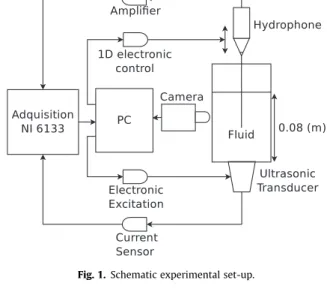
The experimental set-up consists of a cylindrical vessel of 90 mm inner diameter and 150 mm height, built in 5 mm thick
borosilicate glass (Fig. 1). The vessel is filled with 500 ml of fluid, resulting in a level of 80 mm. The fluid is insonified by an 19.7 kHz transducer located at the bottom of the vessel. The radi-ant face of the transducer has a diameter d = 50 mm. Because the studied phenomena is highly temperature-dependent, and cavita-tion noticeably heats the liquid, a special excitacavita-tion strategy was developed to avoid excessive heating of the liquid: ultrasound is turned on during about 2000 cycles, after which the system is left still during 6 s. Preliminary trials have established that this strat-egy allows the realization of cavitation experiments while keeping the temperature constant within 1!C.
The emitter amplitude was characterized by monitoring the peak displacement U0of the transducer during the experiments.
The latter can be obtained by monitoring the current I feeding the transducer, and a calibration curve of U0vs. Iwas drawn. The
current I was measured using a high frequency Hall-effect probe, while the displacement of the transducer radiant face U0was
mea-sured with a laser-Doppler system. The resulting calibration curve is shown inFig. 2. It can be seen that the relationship between U0
and I is quite linear, and we checked that this linear relationship remained unchanged even if the impedance loading the transducer was varied. This justifies our method to monitor the displacement amplitude of the transducer face during the experiments.
On the other hand, the acoustic pressure in the chamber was measured with a home-made PVDF hydrophone[35], which was calibrated by using a non-linear calibration system [36]. The sensitivity of the probe at the fundamental frequency was found
Fig. 1. Schematic experimental set-up.
0 0.2 0.4 0.6 0.8 1 0 1 2 3 4 5 6
I
RMS(A)
U
0(µ
m
)
to be 0:66 $ 0:02
l
V=Pa. The probe can be displaced within 0.02 mm in the whole cavitation chamber along the radial and axial directions, with a motorized translation stage controlled by the general management system of the experiment.The fluid was imaged by a high speed camera (Phantom M310) allowing 2000 frames per second (FPS) at full resolution. The cam-era was disposed in front of the vessel, as shown inFig. 1.
The experimental setup was controlled by a LabView program in such a way that once the excitation amplitude reached an estab-lished level, a signal was generated, to trigger the acquisitions of the image. The transducer feed current and the acoustic pressure level was digitized by a National Instrument PCI-6133 acquisition card of 2 MS/s sampling rate and 14 bit resolution.
3. Experiment
The viscosity of the liquid was varied by adding Polyethylene Glycol of 8000 g/mol molar mass (PEG-8000) in distilled water. This method allows a precise control of the mixture viscosity with-out altering noticeably its density[37]. The viscosities of the mix-tures used in our experiments were measured with a rheometer (Physica MCR301) and are reported inTable 1.
Since cavitation is sensitive to surface tension and to the dis-solved air content, we checked whether both properties were affected by the presence of PEG in water. We found such properties only for PEG 6000 in the literature. For the latter, at our largest concentration (w ¼ 0:1) and at 20 !C, surface tension falls down to 60 mN m%1(compared to 73 mN m%1for pure water)[39], and
the dissolved oxygen content falls decreases to 91% of its value in pure water. Although the change this constitutes a noticeable change for both physical properties, we expect that the effects of the presence of PEG on the cavitation field are due essentially to the viscosity increase.
The same experimental protocol was repeated for the four dif-ferent liquids, and varying the displacement amplitudes of the transducer tip U0in the range of [1.78–6.49]
l
m.The axial variation of the acoustic pressure was recorded by mov-ing the hydrophone by 1 mm steps along the symmetry axis (Z direc-tion), and the RMS pressure level was extracted at each location. To ensure that the RMS values reported were not biased, we use the fol-lowing protocol. At each location, a sample of 250 ms duration was recorded (Fig. 3a). The recording was started 100 ms before the trig-ger signal was received from the transducer, in order to ensure that the rising transient was correctly measured. Moreover, since the transducer is switched on for only 100 ms, a recording duration of 250 ms also ensured that the transient decay of the acoustic field was also recorded, as shown inFig. 3. Both the rising and decay tran-sients were found to last for about tens of periods (Fig. 3b and c), except for some occasions, especially near the pressure antinodes, where the ring-down of the signal could last for about 1 s. A specific algorithm was designed to eliminate the transients in the calcula-tion of the RMS value. Finally, the standard deviacalcula-tion on the RMS pressure level was found to reach 110 kPa in the worst case.
In parallel, for each experiment, an image of the cavitation chamber was recorded in order to visualize the bubble structures obtained.
4. Results 4.1. Distilled water
Fig. 4shown the acoustic pressure profile along the Z direction for different displacement amplitudes.
For low emitter amplitudes (blue star and green diamond curves), the acoustic pressure field shows a local minimum at approximately 25 mm from the transducer face, and a local maxi-mum at about 45 mm. For convenience, such pressure profiles will be called hereinafter as a ‘‘standing wave’’ profile, as soon as it exhibits a marked pressure minimum, which we will loosely term as ‘‘pressure node’’.
For emitter amplitudes greater than or equal to 3.98
l
m, the pressure profile gradually becomes nearly monotonic, and the standing wave character disappears, although small local maxima are still visible. More interestingly, increasing the emitter ampli-tude yields a decrease of the whole acoustic pressure profile. This behavior is a sign of self-attenuation of the wave, which hasTable 1
Viscosity and density of a mixture as a function of the concentration of PEG-8000 in water.
Mass ratio w ¼ mPEG
mPEGþmH2O Viscositym(mPa s) Densityq(kg/m
3)
0.00 1.0a 998.2a
0.03 4.7 ± 0.1 960 ± 60 0.06 6.2 ± 0.1 980 ± 49 0.10 9.0 ± 0.1 978 ± 25 a Value from Ref.[38]
0 0.05 0.1 0.15 0.2 0.25 −4 −2 0 2 4 x 10⁵ Time (s) Pressure (Pa) 0.0905 0.091 0.0915 −2 −1 0 1 2 x 10⁵ Time (s) Pressure (Pa) 0.2085 0.209 0.2095 −2 −1 0 1 2x 10 5 Time (s) Pressure (Pa)
c
b
a
Fig. 3. a: Typical sample of the acoustic pressure versus time. The transducer is switched on near 90 ms. b: Zoom on the rising of the hydrophone signal. c: Zoom on the decay of the hydrophone signal.
already been described for cone bubble structures[5]and was pre-dicted theoretically in Ref.[27].
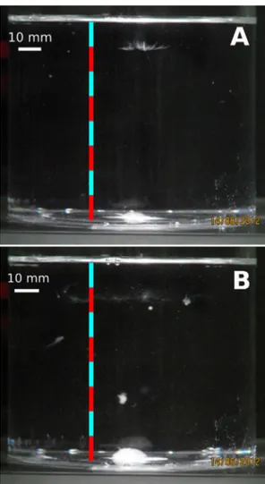
Simultaneously, pictures of the bubble structures in the cavita-tion chamber were recorded for several values of the emitter amplitude.Fig. 5shows snapshots of the liquid for weak emitter amplitudes (U0¼ 1:78
l
m and 2:57l
m). It can be appreciated thatno large structure is formed yet, and only a small ‘‘spherical cap’’-shaped structure forms on the transducer surface, centered on the symmetry axis of the vessel. OnFig. 5A, a small filamentary structure also appears at about 10 mm below the liquid free sur-face, looking like a starfish-structure[2]. Moreover, on the image ofFig. 5B, a small bubble cloud is visible as a large white dot at about 25 mm above the transducer. This structure looks like a bub-ble cluster, which is known to behave as a single large bubbub-ble[2]. Since the size of this cluster is clearly above the resonance radius at 19.7 kHz (Rres¼ 140
l
m), it must be attracted by the Bjerknes forcetoward a pressure node, which is indeed present at this location (see green diamond symbols curve onFig. 4). Moreover, the star-fish visible onFig. 5A appears to have widened onFig. 5B and is located slightly deeper.
Fig. 6shows the bubble distributions for larger emitter ampli-tudes. For U0¼ 5:53
l
m, (Fig. 6A), a new ‘‘tree-like’’ structureappears, formed by a thick vertical filament seeming to originate from the center of the transducer, enriched laterally by densely distributed bubble filaments, so that the whole appears as the ‘‘trunk’’ of a tree. As the emitter amplitude is further increased, the structure gradually extends in height and for U0P 6:23
l
m,attains a quasi stationary shape of approximately 20 mm diameter and 60 mm height (Fig. 6B). It is reminiscent of the so-called ‘‘flare’’ structure described by Mettin [2] as originating from a conical structure near the vibrating wall, from which bubbles stream far away from the transducer forming a broad path, ending up as a large filamentary structure.
Finally, comparison with the pressure profiles ofFig. 4 shows that the appearance of this structure coincides with the transition from a standing wave-like to a monotonically decreasing pressure profile, and that the structure growth in height coincide with a glo-bal decrease of the pressure profile (see curves from U0¼ 3:98
l
mto U0¼ 6:49
l
m inFig. 4). This will be discussed below.4.2. Water–PEG mixtures
Figs. 7–9display the axial pressure profiles obtained in experi-ments with the different water–PEG mixtures, trying to keep con-stant the emitter amplitude for the different liquids. The profiles
measured for pure water (
l
l¼ 1:0 mPa s) are recalled forcompar-ison (blue star symbols curves).
For a low emitter amplitude, (U0in the range [2.10–3.14]
l
m),Fig. 7 shows that regardless of the viscosity value, the acoustic pressure profile exhibits a standing wave-like shape, with a local minimum located at a distance ranging between 20 and 30 mm from the transducer tip.
In the range of medium emitter amplitudes (U0 in [5.13–
5.26]
l
m), two types of acoustic pressure profiles were found (Fig. 8). For the lowest liquid viscosities (l
l¼ 1:0 and 4.7 mPa s),the pressure profile has evolved into a monotonic shape (blue stars and green diamonds curves). Conversely, for large fluid viscosities (
l
l¼ 6:2 and 9.0 mPa s), the acoustic pressure still displays astanding wave behavior (red circles and light-blue squares symbols inFig. 8).
Finally, increasing more the driving amplitude, the standing wave shape evolves into a monotonic wave profile, for all viscosi-ties (Fig. 9). Interestingly, and counter-intuitively, the latter figure also shows that once the pressure profile has switched to a monotonic shape, the higher the viscosity, the higher the global amplitude of the pressure profile.
By observing the images of the bubble structures for all exper-iments, we found that the above-described transition from a stand-ing wave to a monotonic pressure profile always matches the appearance of the large flare-like bubble structure. There seems therefore to be a universal correlation between the disappearance
0 10 20 30 40 50 60 70 80 0 0.5 1 1.5 2 2.5 3 x 10⁵ Distance to transducer (mm) Pressure (Pa) U0=1.78 µm U0=2.57 µm U0=3.98 µm U0=5.53 µm U0=6.23 µm U0=6.49 µm
Fig. 4. Axial acoustic pressure profile for different excitation levels in pure water. (For interpretation of the references to color in this figure caption, the reader is referred to the web version of this article.)
Fig. 5. Bubble structures in the cavitation chamber for experiments with pure water, for low emitter amplitudes (U0<3:98lm). A: U0¼ 1:78lm; B: U0¼ 2:57lm. A centimeter vertical scale has been added for readability.
of the standing waves and the appearance of the large structure. This feature had already been recognized by Campos-Pozuelo and co-workers for the cone bubble structure (see Fig. 6 in Ref.[5]). The transition occurs above a threshold amplitude of the trans-ducer, and the present results show that increasing the liquid vis-cosity shifts this threshold toward large amplitudes.
5. Discussion 5.1. Bubble structures
The above experimental results are qualitatively consistent with the interpretation suggested by the model and simulations in Refs.[27,29]. It was proposed that the transition to a monotonic pressure profile occurs because the appearance of a dense bubble population near the transducer yields a large energy dissipation, by the mechanism recalled in Section1. The energy dissipated by the bubbles damps the emitted wave and prohibits the formation of longitudinal standing waves in absence of sufficiently large reflected waves. This results in a damped traveling wave near the transducer, which strongly expels the bubble from the transducer by the primary Bjerknes force[2,28,29]. However, pressure antin-odes can still appear far from the emitter, because a sufficient part of the incident wave survives the damping near the emitter and undergoes reflections on the vessel walls or on the free surface. Moreover, the wave may be traveling in the axial direction and standing in the radial direction [28]. This mixture of traveling and standing waves has been conjectured to be responsible for the formation of flare structures[2], and was satisfactorily caught by the model of Ref.[29]. Such a structure is visible for example in
Fig. 6B: basically, the foot of such structures is composed of bub-bles expelled from the transducer by a traveling wave, which ends up in a filamentary structure around a pressure antinode.
In the present case, the detailed comparison between the images of bubble structures and the pressure profiles allow to refine the above interpretation. Comparing for example Fig. 6A
Fig. 6. Bubble structures in the cavitation chamber for experiments with pure water, for high emitter amplitudes. A: U0¼ 5:53lm, tree-like structure: between z ¼ 2 cm and z ¼ 4 cm, the axis is free of bubbles; B: U0¼ 6:49lm, flare-like structure[2]: the major part of the axis is populated with bubbles. The structures ends up as a large streamer. A centimeter vertical scale has been added for readability. 0 10 20 30 40 50 60 70 80 0 0.5 1 1.5 2 2.5 x 10⁵ Distance to transducer (mm) Pressure (Pa) µl = 1.0 mPa ⋅ s µl = 4.7 mPa ⋅ s µl = 6.2 mPa ⋅ s µl = 9.0 mPa ⋅ s
Fig. 7. Axial acoustic pressure profile in water–PEG mixtures of different viscosities. The emitter amplitude ranges between 2.10 and 3.14lm.
0 10 20 30 40 50 60 70 80 0 0.5 1 1.5 2 2.5 3 x 10⁵ Distance to transducer (mm) Pressure (Pa) µl = 1.0 mPa ⋅ s µl = 4.7 mPa ⋅ s µl = 6.2 mPa ⋅ s µl = 9.0 mPa ⋅ s
Fig. 8. Axial acoustic pressure profile in water–PEG mixtures of different viscosities. The emitter amplitude ranges between 5.13 and 5.26lm.
0 10 20 30 40 50 60 70 80 0 0.5 1 1.5 2 2.5 3 x 10⁵ Distance to transducer (mm) Pressure (Pa) µl = 1.0 mPa ⋅ s µl = 4.7 mPa ⋅ s µl = 6.2 mPa ⋅ s µl = 9.0 mPa ⋅ s
Fig. 9. Axial acoustic pressure profile in water–PEG mixtures of different viscosities. The emitter amplitude ranges between 6.29 and 6.40lm.
and B, one could naively think that the structure growth for increasing emitter amplitudes is due to a corresponding global increase of the acoustic pressure field. Comparison of the pressure profile for U0¼ 5:53
l
m (light-blue squares curve onFig. 4) withthe one for U0¼ 6:49
l
m (yellow + signs curve onFig. 4) showsthat the opposite holds. There are therefore more bubbles on the symmetry axis inFig. 6B than on6A because acoustic pressures are lower in B. This could be explained by recalling that in a stand-ing wave, the Bjerknes force on inertial bubbles changes sign above 1.7 bar, and becomes directed towards low acoustic pressures
[40,20,41,42]. This is supported byFig. 6A, which shows that the trunk of the structure exhibits a void region between 20 mm and 40 mm from the transducer. The corresponding pressure profile on Fig. 4 (light-blue squares curves) shows that in this region, the acoustic pressure ranges between 1.5 and 2 bar, and we conjec-ture that the Bjerknes force in this zone repels the bubbles out of axis, up to the small filamentary structure visible at 40 mm above the transducer where the Bjerknes force again attracts the bubbles on the axis.
In the near-transducer zone, fresh bubbles are continuously nucleated on the transducer and strongly expelled upwards by the large Bjerknes force induced by the traveling wave in this region. However, for U0¼ 5:53
l
m (light-blue curve inFig. 4, andstructureFig. 6.A) the acoustic pressure on the axis in this region is larger than 1.7 bar, so that these bubbles should also undergo a radial force pushing them out-of-axis, if one assumes a standing wave in the r-direction. One may therefore expect that the bubbles born on the transducer would also bypass the axis and leave a void region near the transducer. This is not the case probably because the Z-directed expelling Bjerknes force, induced by the traveling wave, is much larger than the R-directed repelling one, induced by the radial standing wave. This simplistic interpretation might however miss some non-stationary mechanisms, and the competi-tion between the radial and axial forces may explain the observa-ble chaotic bending of the structure on a time-scale of the order of the second.
Conversely in Fig. 6B, the whole axis is a bubble attractor because the acoustic pressure is everywhere lower than 1.7 bar (yellow + signs curve onFig. 4). The bubbles launched from the emitter thus follow more or less the axis and the structure appears straighter. It ends up at about 50–60 mm of the transducer, prob-ably because the acoustic pressure becomes lower than the Blake threshold above this point.
A video at 2000 FPS showing the details of the structure dynam-ics for U0’ 6
l
m in pure water is proposed as supplementarymaterial. The structure observed corresponds more or less to the situation ofFig. 6A, and the motion of the bubbles tends to confirm the main lines of the above interpretation.
To summarize, we therefore infer the following qualitative sce-nario to explain the present results:
1. For very low amplitudes, acoustic pressures are high enough to produce inertial bubbles only near the transducer, forming a spherical cap structure, growing with amplitude. A standing wave is present in the whole vessel.
2. Above some threshold, which increases with the liquid viscos-ity, the bubbles near the transducer dissipate enough energy to damp the wave noticeably and produce locally a traveling wave. The resulting Bjerknes force expels the bubbles from the transducer, yielding the trunk of the structure. The pressure values on the axis are high enough to produce an out-of-axis repelling Bjerknes force, which produces a void region on the axis at a given distance from the transducer.
3. As the amplitude is still increased, a larger number of bubbles near the transducer dissipate more energy, yielding a global decrease of the pressure profile. The void regions progressively
disappear as the axis becomes attractive again, so that the structure thus builds up over that part of the axis where the acoustic pressure is higher than the Blake threshold.
5.2. Effect of viscosity
Our experiments show that increasing the liquid viscosity shifts the transitions 1 ! 2 and 2 ! 3 towards higher driving amplitudes in the above scenario. This is consistent with the observed ordering of the curves inFig. 9. At a given driving amplitude, the largest vis-cosity pressure profile is still in phase 2 (light-blue squares curve), whereas the low-viscosity ones are already in phase 3. This results in somewhat counter-intuitive situations where, as exemplified in
Fig. 9, an increase of viscosity results in a globally higher acoustic pressure field.
This suggests a yet unknown mechanism increasing the acous-tic transparency of the cavitating liquid for increasing liquid vis-cosities. Such an effect can be found in fact within the frame of the single bubble physics. Indeed, for large viscosities, the bubble oscillations become so damped that the radial velocity strongly decreases[43], thus reducing the power dissipated by the bubble [Eq. (1)]. We have examined quantitatively this hypothesis in A
and conclude that for the moderate viscosities considered here, it can be discarded.
The precise mechanism by which these transitions occur remains to be explained, especially why, once the flare-like structure is formed, an increase in the emitter amplitudes pro-duces a global decrease of the pressure profile, and why this phenomenon is delayed when increasing the liquid viscosity. One might conjecture an effect of the bubble number and/or size distribution, which is clearly not caught by Louisnard’s model
[27]. By the way, we have tried to apply the latter to the present geometry, carefully accounting for the vibrations of the vessel walls, and adjusting the bubble number (constant above the Blake threshold [27,29]) in order to fit the observations). Some similarities were found, and for example the spherical cap struc-ture could be easily obtained. Nevertheless, the experimentally observed shape of the flare-like structure could not be reason-ably reproduced, and more important, the orders of magnitude of the calculated acoustic pressures were lower than the ones measured here, except in the immediate vicinity of the trans-ducer. This suggest that Louisnard’s model overestimates in some way the attenuation of the field, and we conjecture that this is due to the constant bubble density hypothesis, which must therefore be refined. The present results thus show that a fully predictive model of acoustic cavitation is not yet achieved. Measuring acoustic pressure fields in simple experi-mental geometries, like the present one, constitutes a good benchmark for model enhancements. Moreover, our results show that the liquid viscosity has a noticeable influence on the fields observed, and new or existing models should demonstrate their ability to catch this effect reasonably well.
Acknowledgments
This work was supported by a Chilean Fondo de Fomento al Desarrollo Científico y Tecnológico (FONDEF), project D09I1235 and by Comisión Nacional de Investigación Científica y Tecnológica (CON-ICYT), project ‘‘Apoyo a la realización de Tesis Doctoral 2012’’ number 24121209. O. Louisnard would also like to acknowledge the sup-port of the French Agence Nationale de la Recherche (ANR), under grant SONONUCLICE (ANR-09-BLAN-0040–02) ‘‘Contrôle par ultra-sons de la nucléation de la glace pour l’optimisation des procédés de congélation et de lyophilisation’’.
Appendix A. Power dissipated by a single bubble as a function of viscosity
We estimate the period-average power dissipated by the radial motion of a bubble, because of viscous friction in the liquid[27]:
P
v¼1TZ T
0 16
pl
lR _R2dt ðA:1Þ
for a given bubble in liquids of different viscosities. The model used to calculate bubble dynamics is the same as in Ref.[27]and is based on a Keller equation complemented by equations accounting for heat and water transfer inside the bubble with approximate diffu-sion layers[44,45]. We consider an air bubble of ambient radius R0¼ 5
l
m excited by a sinusoidal forcing p ¼ p0% pasinð2p
ftÞ, atf ¼ 20 kHz. The liquid is considered at ambient pressure (p0¼ 101; 300 Pa), ambient temperature (T0¼ 20'C), and its
phys-ical properties are the one of water (
q
l¼ 1000 kg/m3,r
= 0.0725 N m%1), except that the viscosity is varied between oneand hundred-fold the viscosity of pure water (
l
w= 10%3Pa s).Fig. A.10displays the results obtained forPvgiven by Eq.(A.1).
For the three lowest viscosities
l
w (blue solid line), 5l
w (greendashed line) and 10
l
w(red dash-dotted line), the behavior is thesame as depicted in Ref.[27]: the dissipated power undergoes a huge jump at the Blake threshold, to reach values orders of magni-tude above the linear prediction. The respective locations of the three curves is intuitive for all values of the driving field: increas-ing viscosity increases viscous dissipation.
For liquid viscosities of 50
l
w (purple square symbols) and100
l
w(black circle symbols), the transition near the Blakethresh-old is smoother. More interesting, there exists a range of acoustic pressures above the Blake threshold where an increase of liquid viscosity yields a decrease of the power dissipated by the bubble. Although this result may sound counter-intuitive, this occurs because a large increase of viscosity strongly damps the bubble dynamics and therefore the velocity gradients in the liquid. Thus, even if
l
lis higher, the integral(A.1)decreases because _R2is muchsmaller over the whole acoustic cycle. This would suggest that very viscous liquids subject to cavitation might be more transparent to acoustic waves in some occasion, because the bubbles they pro-duce undergo less violent oscillations. However, for the viscosities used in the present experiments (less than ten-fold the viscosity of pure water), Fig. A.10 shows that the dissipated power always increases with viscosity (see solid, dashed and dash-dotted lines), and that such a mechanism can be discarded.
Appendix B. Supplementary data
Supplementary data associated with this article can be found, in the online version, at http://dx.doi.org/10.1016/j.ultsonch.2014. 07.007.
References
[1]T.J. Leighton, The Acoustic Bubble, Academic Press, London, 1994.
[2]R. Mettin, Bubble structures in acoustic cavitation, in: A.A. Doinikov (Ed.),
Bubble and Particle Dynamics in Acoustic Fields: Modern Trends and
Applications, Research Signpost, Kerala (India), 2005, pp. 1–36.
[3]A. Moussatov, C. Granger, B. Dubus, Cone-like bubble formation in ultrasonic
cavitation field, Ultrason. Sonochem. 10 (2003) 191–195.
[4] A. Moussatov, R. Mettin, C. Granger, T. Tervo, B. Dubus, W. Lauterborn, Evolution of acoustic cavitation structures near larger emitting surface, in: Proceedings of the World Congress on Ultrasonics, Paris (France), 2003, pp. 955–958.
[5]C. Campos-Pozuelo, C. Granger, C. Vanhille, A. Moussatov, B. Dubus,
Experimental and theoretical investigation of the mean acoustic pressure in
the cavitation field, Ultrason. Sonochem. 12 (2005) 79–84.
[6]B. Dubus, C. Vanhille, C. Campos-Pozuelo, C. Granger, On the physical origin of
conical bubble structure under an ultrasonic horn, Ultrason. Sonochem. 17
(2010) 810–818.
[7]H. Xu, N.C. Eddingsaas, K.S. Suslick, Spatial separation of cavitating bubble
populations: the nanodroplet injection model, J. Am. Chem. Soc. 131 (2009)
6060–6061.
[8]H. Xu, N.G. Glumac, K.S. Suslick, Temperature inhomogeneity during
multibubble sonoluminescence, Angew. Chem. Int. Ed. 49 (2010) 1079–1082.
[9]R. Mettin, From a single bubble to bubble structures in acoustic cavitation, in:
T. Kurz, U. Parlitz, U. Kaatze (Eds.), Oscillations, Waves and Interactions,
Universitätsverlag Göttingen, 2007, pp. 171–198.
[10]L.L. Foldy, The multiple scattering of waves, Phys. Rev. 67 (3–4) (1944) 107–
119.
[11]E. Silberman, Sound velocity and attenuation in bubbly mixtures measured in
standing wave tubes, J. Acoust. Soc. Am. 29 (8) (1957) 925–933.
[12]K.W. Commander, A. Prosperetti, Linear pressure waves in bubbly liquids:
comparison between theory and experiments, J. Acoust. Soc. Am. 85 (2) (1989)
732–746.
[13]L.D. Rozenberg, The cavitation zone, in: L.D. Rozenberg (Ed.), High-intensity
Ultrasonic Fields, Plenum Press, New-York, 1971.
[14]M.M. van Iersel, N.E. Benes, J.T.F. Keurentjes, Importance of acoustic shielding
in sonochemistry, Ultrason. Sonochem. 15 (4) (2008) 294–300.
[15]T.G. Leighton, Bubble population phenomena in acoustic cavitation, Ultrason.
Sonochem. 2 (2) (1995) S123–S136.
[16]L. van Wijngaarden, On the equations of motion for mixtures of liquid and gas
bubbles, J. Fluid Mech. 33 (3) (1968) 465–474.
[17]V.N. Alekseev, V.P. Yushin, Distribution of bubbles in acoustic cavitation, Sov.
Phys. Acoust. 32 (6) (1986) 469–472.
[18]Y.A. Kobelev, L.A. Ostrovskii, Nonlinear acoustic phenomena due to bubble
drift in a gas–liquid mixture, J. Acoust. Soc. Am. 85 (2) (1989) 621–629.
[19]I. Akhatov, U. Parlitz, W. Lauterborn, Pattern formation in acoustic cavitation, J.
Acoust. Soc. Am. 96 (6) (1994) 3627–3635.
[20]U. Parlitz, R. Mettin, S. Luther, I. Akhatov, M. Voss, W. Lauterborn, Spatio
temporal dynamics of acoustic cavitation bubble clouds, Philos. Trans. R. Soc.
Lond. A 357 (1999) 313–334.
[21] R. Mettin, J. Appel, D. Krefting, R. Geisler, P. Koch, W. Lauterborn, Bubble structures in acoustic cavitation: observation and modelling of a jellyfish-streamer, in: Special Issue of the Revista de Acustica, Forum Acusticum Sevilla, Spain, 16–20 Sept. 2002, vol. XXXIII, Sevilla, Spain, 2002, pp. 1–4.
[22]J. Appel, P. Koch, R. Mettin, W. Lauterborn, Stereoscopic high-speed recording
of bubble filaments, Ultrason. Sonochem. 11 (2004) 39–42.
[23]O. Louisnard, Contribution à l’étude de la propagation des ultrasons en milieu
cavitant, Thèse de doctorat, Ecole des Mines de Paris, Paris, France, 1998.
[24]C. Vanhille, C. Campos-Pozuelo, Nonlinear ultrasonic propagation in bubbly
liquids: a numerical model, Ultrasound Med. Biol. 34 (5) (2008) 792–808.
[25]C. Vanhille, C. Campos-Pozuelo, Numerical simulations of three-dimensional
nonlinear acoustic waves in bubbly liquids, Ultrason. Sonochem. 20 (3) (2013)
963–969.
[26]I. Tudela, V. Sáez, M.D. Esclapez, M.I. Díez-García, P. Bonete, J. González-García,
Simulation of the spatial distribution of the acoustic pressure in sonochemical reactors with numerical methods: a review, Ultrason. Sonochem. 21 (3) (2014)
909–919.
[27]O. Louisnard, A simple model of ultrasound propagation in a cavitating liquid.
Part I: theory, nonlinear attenuation and traveling wave generation, Ultrason.
Sonochem. 19 (2012) 56–65.
[28]P. Koch, R. Mettin, W. Lauterborn, Simulation of cavitation bubbles in
travelling acoustic waves, in: D. Cassereau (Ed.), Proceedings CFA/DAGA’04
Strasbourg, DEGA Oldenburg, 2004, pp. 919–920.
[29]O. Louisnard, A simple model of ultrasound propagation in a cavitating liquid.
Part II: primary bjerknes force and bubble structures, Ultrason. Sonochem. 19
(2012) 66–76.
[30]A. Prosperetti, Thermal effects and damping mechanisms in the forced radial
oscillations of gas bubbles in liquids, J. Acoust. Soc. Am. 61 (1) (1977) 17–27.
Fig. A.10. Power dissipated by a 5lm air bubble driven by a 20 kHz acoustic field of amplitude pa, for liquid viscosities N times larger than the viscosity of waterlw(N = 1, 5, 10, 50 and 100). (For interpretation of the references to color in this figure caption, the reader is referred to the web version of this article.)
[31]J.A. Venegas-Sanchez, T. Motohiro, K. Takaomi, Ultrasound effect used as external stimulus for viscosity change of aqueous carrageenans, Ultrason.
Sonochem. 20 (4) (2013) 1081–1091.
[32]S. Pilli, P. Bhunia, S. Yan, R.J. LeBlanc, R.D. Tyagi, R.Y. Surampalli, Ultrasonic
pretreatment of sludge: a review, Ultrason. Sonochem. 18 (1) (2011) 1–18.
[33]A. Grönroos, P. Pirkonen, H. Kyllönen, Ultrasonic degradation of aqueous
carboxymethylcellulose: effect of viscosity, molecular mass, and
concentration, Ultrason. Sonochem. 15 (4) (2008) 644–648.
[34]N.C. Eddingsaas, K.S. Suslick, Evidence for a plasma core during multibubble
sonoluminescence in sulfuric acid, J. Am. Chem. Soc. 129 (2007) 3838–3839.
[35]L. Gaete-Garretón, Y. Vargas-Hernández, S. Pino-Dubreuil, F. Montoya-Vitini,
Ultrasonic detectors for high-intensity acoustic fields, Sens. Actuators A: Phys.
37–38 (1993) 410–414.
[36]L. Gaete-Garretón, Y.V. Hernández, F. Montoya-Vitini, J.A. Gallego-Juárez, A
simple non-linear technique for secondary calibration of ultrasonic probes,
Sens. Actuators A: Phys. 69 (1) (1998) 68–71.
[37]P. Gonzalez-Tello, F. Camacho, G. Blazquez, Density and viscosity of
concentrated aqueous solutions of polyethylene glycol, J. Chem. Eng. Data 39
(3) (1994) 611–614.
[38] R.W. Johnson (Ed.), The Handbook of Fluid Dynamics, Idaho National Engineering and Environmental Lab., 1998.
[39] M. Mazandarani, A. Eliassi, M. Fazlollahnejada, Experimental data and correlation of surface tension of binary polymer solutions at different temperatures and atmospheric pressure, in: European Congress of Chemical Engineering (ECCE-6), Copenhagen, 2007.
[40] I. Akhatov, R. Mettin, C.D. Ohl, U. Parlitz, W. Lauterborn, Bjerknes force
threshold for stable single bubble sonoluminescence, Phys. Rev. E 55 (3)
(1997) 3747–3750.
[41]T.J. Matula, Inertial cavitation and single-bubble sonoluminescence, Philos.
Trans. R. Soc. Lond. A 357 (1999) 225–249.
[42] O. Louisnard, Analytical expressions for primary Bjerknes force on inertial cavitation bubbles, Phys. Rev. E 78 (3) (2008) 036322, http://dx.doi.org/
10.1103/PhysRevE.78.036322.
[43]S. Hilgenfeldt, M.P. Brenner, S. Grossman, D. Lohse, Analysis of Rayleigh–
Plesset dynamics for sonoluminescing bubbles, J. Fluid Mech. 365 (1998) 171–
204.
[44]R. Toegel, B. Gompf, R. Pecha, D. Lohse, Does water vapor prevent upscaling
sonoluminescence?, Phys Rev. Lett. 85 (15) (2000) 3165–3168.
[45]B.D. Storey, A. Szeri, A reduced model of cavitation physics for use in