Pour l'obtention du grade de
DOCTEUR DE L'UNIVERSITÉ DE POITIERS École nationale supérieure d'ingénieurs (Poitiers)
Laboratoire d'informatique et d'automatique pour les systèmes - LIAS (Poitiers) (Diplôme National - Arrêté du 25 mai 2016)
École doctorale : Sciences et ingénierie pour l'information, mathématiques - S2IM (Poitiers) Secteur de recherche : Image, signal et automatique
Présentée par :
Ziad Alkhoury
Minimality, input-output equivalence and identifiability of
LPV systems in state-space and linear fractional
representations
Directeur(s) de Thèse :Guillaume Mercère, Mihaly Petreczky Soutenue le 09 novembre 2017 devant le jury
Jury :
Président Thierry Poinot Professeur, LIAS, ENSIP, Université de Poitiers Rapporteur Xavier Bombois Directeur de recherche CNRS, École centrale de Lyon Rapporteur Herbert Werner Professor, Technische Universität Hamburg, Deutschland Membre Guillaume Mercère Maître de conférences, LIAS, ENSIP, Université de Poitiers Membre Mihaly Petreczky Chargé de recherche, CRIStAL, Université de Lille
Membre Marion Gilson Professeur, CRAN, Université de Lorraine, Nancy
Membre Roland Toth Professor, Eindhoven University of Technology, Netherlands
Pour citer cette thèse :
Ziad Alkhoury. Minimality, input-output equivalence and identifiability of LPV systems in state-space and linear
fractional representations [En ligne]. Thèse Image, signal et automatique. Poitiers : Université de Poitiers, 2017.
DOCTEUR DE L’UNIVERSITE DE POITIERS (Diplôme National - Arrêté du 25 mai 2016)
Ecole Doctorale: Sciences et Ingénierie pour l’Informations, Mathématiques Secteur de Recherche : Image, Signal et Automatique
Présentée par
ZIAD ALKHOURY
_________________________________________________________________
Minimality, input-output equivalence and identifiability of
LPV systems in State-Space and Linear Fractional
Representations
_________________________________________________________________ Directeur de thèse : Guillaume MERCÈRE Université de Poitiers, LIAS Co-encadrant : Mihály PETRECZKY Ecole Centrale de Lille, CRIStAL
2017
COMPOSITION DU JURY :
Présidente : Marion GILSON - Professeur des Universités Université de Lorraine, CRAN Rapporteurs : Herbert WERNER - Professeur des Universités
Hamburg University of Technology Xavier BOMBOIS - Directeur de Recherche
Ecole Centrale de Lyon, Ampère Examinateurs : Thierry POINOT - Professeur des Universités
Université de Poitiers, LIAS
Roland TÓTH - Maître de conférences
Eindhoven University of Technology Guillaume MERCÈRE - Maître de conférences, HdR
Université de Poitiers, LIAS Mihály PETRECZKY - Chargé de Recherche
Ecole Centrale de Lille, CRIStAL
Thèse préparée au sein du Labaratoire d’Informatique et d’Automatique pour les Systèmes de Poitiers et du Departement d’Informatique et Automatique d’IMT Lille Douai
SCIENCES ET INGÉNIERIE POUR L’INFORMATIONS, MATHÉMATIQUES
Ph.D. T H E S I S
to obtain the title of
Doctor of Science
of the University of Poitiers
Prepared byZiad ALKHOURY
_________________________________________________________________
Minimality, input-output equivalence and identifiability of
LPV systems in State-Space and Linear Fractional
Representations
_________________________________________________________________ Advisors:
Guillaume MERCÈRE, Ph.D., HdR.
The Laboratory of Computer Science and Automatic Control for Systems (LIAS),
UNIVERSITY OF POITIERS
Mihály PETRECZKY, Ph.D.
The French National Center for Scientific Research (CNRS), Centre de Recherche en Informatique, Signal et Automatique de Lille
(CRIStAL), UMR CNRS 9189, École Centrale de Lille.
prepared at: LIAS, Université de Poitiers & DIA, IMT Lille Douai 2017
Abstract vii
Résumé ix
Abbreviations xi
Notations xiii
List of Figures xvii
1 Introduction 1
1.1 System identification. . . 3
1.2 Motivation and contributions . . . 5
1.3 Outline of the thesis . . . 7
1.4 Publications . . . 8
2 Background and problem formulation 9 2.1 Introduction . . . 9
2.2 State-space representation of LTI systems . . . 12
2.3 Representations of LPV systems. . . 15
2.3.1 State-space representation of LPV systems. . . 16
2.3.2 State-space representation with affine dependence of LPV systems . . . 18
2.3.3 Linear fractional representation of LPV systems . . . 20
2.3.4 Equivalence between Linear Fractional Representation and State-Space Representation of LPV systems . . . 22
2.4 Theoretical challenges in LPV system identification . . . 23
2.4.1 Identifiability of Affine-LPV models . . . 23
2.4.2 Local and global identification techniques . . . 26
2.4.3 The relationship between Linear Fractional representation and Affine-LPV State-Space Representations for LPV systems 29 2.5 Conclusion . . . 33
Appendices of Chapter 2 35 Appendix 2.A Input-output maps vs. the behavioral approach . . . 35
3 Identifiability of Affine-LPV state-space models 37 3.1 Introduction . . . 37
3.2 Affine-LPV systems: some important definitions . . . 40
3.3 Identifiability of Affine-LPV state-space parametrizations. . . 43
3.3.1 Structural identifiability of Affine-LPV parameterizations . . 43
3.3.2 Local structural identifiability of Affine-LPV parametrizations 45 3.3.3 Conditions for identifiability . . . 45
3.4 Illustrative examples . . . 49
3.4.1 Global structural identifiability. . . 49
3.4.2 Global structural identifiability for affine parameterizations. 53 3.4.3 Local structural identifiability . . . 54
3.5 Conclusion . . . 56
Appendices of Chapter 3 57 Appendix 3.A Proof of Lemma 1 . . . 57
Appendix 3.B Proof of Theorem 3 . . . 57
Appendix 3.C Proof of Theorem 4 . . . 58
Appendix 3.D Proof of Lemma 2 . . . 59
Appendix 3.E Proof of Theorem 5 . . . 60
Appendix 3.F Proof of Theorem 6 . . . 62
4 Systematic modeling error for the local identification approach 65 4.1 Introduction . . . 65
4.2 Preliminaries. . . 67
4.3 Systematic error characterization . . . 71
4.3.1 General bound . . . 71 4.3.2 Special cases . . . 72 4.3.3 Basic trade-offs. . . 74 4.4 Illustrative examples . . . 74 4.5 Conclusion . . . 83 Appendices of Chapter 4 85 Appendix 4.A Proof of Lemma 3 . . . 85
Appendix 4.B Proof of Lemma 4 . . . 85
Appendix 4.C Proof of Theorem 7 . . . 86
Appendix 4.D Proof of Theorem 8 . . . 90
Appendix 4.E Proof of Theorem 9 . . . 90
Appendix 4.F Proof of Theorem 10 . . . 91
Appendix 4.G Proof of Theorem 11 . . . 92
Appendix 4.H Realization theory notions for state-space representation of LTI systems . . . 92
5 The transformation between Affine-LPV and LFR models 95 5.1 Introduction . . . 95
5.2 LFR and the relationship with Affine-LPV models . . . 96
5.2.1 General LFR models as multidimensional systems. . . 97
5.2.2 Transforming Affine-LPV models to LFR ones and vice versa 102 5.2.3 Problem formulation . . . 104
5.3 Equivalence between Affine-LPV and LPV-LFR . . . 104
5.3.1 Matrix full rank factorization . . . 104
5.3.2 Preservation of minimality and input-output behavior . . . . 105
5.3.3 Preservation of structural identifiability . . . 106
Appendices of Chapter 5 111
Appendix 5.A Sketch of the proof of Theorem 19 . . . 111
Appendix 5.B Sketch of the proof of Theorem 20 . . . 113
Appendix 5.C Proof of Corollary 1. . . 114
Appendix 5.D Proof of Corollary 2. . . 114
Appendix 5.E Proof of Theorem 21 . . . 114
Appendix 5.F Sketch of the proof of Theorem 22 . . . 115
6 Conclusions and future work 117
In this thesis, important concepts related to the identification of Linear Parameter-Varying (LPV) systems are studied.
First, we tackle the problem of identifiability of Affine-LPV (ALPV) state-space parametrizations. A new sufficient and necessary condition is introduced in order to verify the structural identifiability for ALPV parameterizations. The identifiability of this class of parameterizations is related to the lack of state-space isomorphisms between any two models corresponding to different parameter values. In addition, we present a sufficient and necessary condition for local struc-tural identifiability, and a sufficient condition for (global) strucstruc-tural identifiability which are both based on the rank of a model-based matrix. These latter conditions allow systematic verification of structural identifiability of ALPV models.
Second, since local identification techniques are inevitable in certain appli-cations, it is necessary to study the discrepancy between different LPV models obtained using different local techniques. We provide an analytic error bound on the difference between the input-output behaviors of any two LPV models which are frozen equivalent. This error bound turns out to be a function of both (i) the speed of the change of the scheduling signal and (ii) the discrepancy between the coherent bases of the two LPV models. In particular, the difference between the outputs of the two models can be made arbitrarily small by choosing a scheduling signal which changes slowly enough.
Finally, we introduce and study important properties of the transformation of ALPV state-space representations into Linear Fractional Representations (LFRs). More precisely, we show that (i) state minimal ALPV representations yield minimal LFRs, and vice versa, (ii) the input-output behavior of the ALPV repre-sentation determines uniquely the input-output behavior of the resulting LFR, (iii) structurally identifiable ALPV models yield structurally identifiable LFR ones, and vice versa. We then characterize LFRs which correspond to equivalent ALPV models based on their input-output maps.
As illustrated all along the manuscript, these results have important conse-quences for identification and control of LPV systems.
Keywords - Linear parameter-varying (LPV) systems, structural properties,
sys-tem identification, minimality, identifiability, input-output equivalence, state-space representation, linear fractional representation (LFR)
Dans cette thèse, plusieurs concepts importants liés à la théorie de la réalisation des modèles linéaires à paramètres variants (LPV) sont étudiés. Tout d’abord, nous abordons le problème de l’identifiabilité des modèles LPV affines (ALPV). Une nouvelle condition suffisante et nécessaire est introduite afin de garantir l’identifiabilité structurelle pour les paramétrages ALPV. L’identifiabilité de cette classe de paramétrages est liée à l’absence d’isomorphismes liant deux représentations d’état LPV lorsque deux modèles LPV correspondant à différentes valeurs des variables de paramétrage sont considérés. Nous présentons ainsi une condition suffisante et nécessaire pour l’identifiabilité structurelle locale, et une condition suffisante pour l’identifiabilité structurelle (globale) qui sont toutes deux fonction du rang d’une matrice définie par l’utilisateur. Ces dernières conditions permettent la vérification de l’identifiabilité structurelle des modèles ALPV.
Ensuite, étant donné que les techniques d’identification dites locales sont parfois inévitables, nous fournissons une expression analytique de la borne supérieure de la différence de comportements entrées-sorties de deux modèles LPV équivalents localement. Cette différence se révèle être une fonction de (i) la vitesse de changement du signal de séquencement et (ii) l’écart entre les bases cohérentes de deux modèles LPV. En particulier, la différence entre les sorties des deux modèles peut être arbitrairement réduite en choisissant un signal de séquencement qui varie assez lentement.
Enfin, nous présentons et étudions des propriétés importantes de la trans-formation des représentations d’état ALPV en Représentations Linéaires Frac-tionnelles (LFR). Plus précisément, nous montrons que (i) les représentations ALPV minimales conduisent à des LFR minimales, et vice versa, (ii) le comporte-ment entrée-sortie de la représentation ALPV détermine de manière unique le comportement entrée-sortie de la LFR résultante, (iii) les modèles ALPV struc-turellement identifiables fournissent des LFRs strucstruc-turellement identifiables et vice versa. Nous caractérisons ensuite les LFRs qui correspondent à des modèles ALPV équivalents basés sur leurs applications entrées-sorties. Comme illustré tout au long du manuscrit, ces résultats ont des conséquences importantes pour l’identification et la commande des systèmes LPV.
Mots clés - systèmes linéaires á paramètres variants (LPV), propriétés
structurels, identification, minimalité, identifiabilité, équivalence entrée-sortie, représentations d’état, représentations Linéaires Fractionnelles (LFR)
LTI Linear Time-Invariant
LPV Linear Parameter-Varying
ALPV Affine Linear Parameter-Varying
IO Input-Output
SS State-Space
IOR Input-Output Representation
SSR State-Space Representation
LFR Linear Fractional Representation
SVD Singular Value Decomposition
LMI Linear Matrix Iequality
LTV Linear Time-Varying
TV Time-Varying
SM Set Membership
SISO Single Input Single Output
MIMO Multi-Input Multi-Output
OE Output Error
PEM Prediction Error Method
LS Least Squares
LS-SVM Least Squares-Support Vector Machine
IOM Input-Output Map
CT Continuous-Time
DT Discrete-Time
TF Transfer Function
LPV-ARX LPV-Auto-Regressive with eXogenous variable (model)
NL Non-Linear
General
N The set of natural numbers R The set of real numbers C The set of complex numbers
UN The set of all functions of the form φ ∶ N → U
③ Complex number
Ib
a The set {a, a + 1, ⋯, b − 1, b}, where a, b ∈ N and a ≤ b
i, j, k, q, v multi-use indexes
In The n × n identity matrix, where n ∈ N
I The identity matrix (with proper dimension) λ Backward shift operator
U The input space
Y The output space
P The scheduling space
X The state space
U The set of input signals Y The set of output signals P The set of scheduling signals X The set of state signals
F Input-output map
YΣ,x0 Input-to-output function of an LPV model Σ, induced by
the initial state x0
XΣ,x0 Input-to-state function of an LPV model Σ, induced by the
initial state x0
YΣ Input-to-output function of an LPV model Σ, induced by
the zero initial state
XΣ Input-to-state function of an LPV model Σ, induced by the
zero initial state
θ The unknown parameters vector Θ The unknown parameters set ○ Function concatenation
⊗ Kronecker product
◇ Evaluation of a coefficient function along a trajectory of p A⊺ Transpose of matrix A
A−1 Inverse of matrix A
vec(A) Vector of the elements of a matrix A GL(n) The set of n× n invertible matrices
ker Kernel
Im Image
det Determinant
diag Diagonal matrix spanx Span of x Norms-related
∥A∥ induced 2- Norm of a matrix A ∥V ∥n nthvector norm of a vector V
∥V ∥∞ Infinity vector norm of a vector V
∥u∥l2 The l2norm of the signal u, i.e.,∥u∥l2 = (∑k=0∥u(k)∥ 2 2)
1 2
∥u∥l∞ The l∞norm of the signal u, i.e.,∥u∥l∞ = supt∈N∥u(t)∥
l2(Rn) The set of square summable sequences taking values in Rn
l∞(U) The set of bounded inputs
L(l2) the set of all bounded operators from l2(R) to l2(R)
L(l2(Rn)) the set of all bounded operators from l2(Rn) to l2(Rn)
Systems
G Real system t The time instant u The input signal y The output signal x The state signal p the scheduling signal
x0 The initial state, i.e., x0= x(0)
nx The dimension of the state vector of state-space models
nu The dimension of the input vector of state-space models
ny The dimension of the output vector of state-space models
np The dimension of the scheduling parameter vector of an
LPV model
LTI systems
▲ An LTI state-space model
❆, ❇, ❈, ❉ The matrices of an LTI state-space model ❚ LTI isomorphism (state transformation)
{▲❚} The set of LTI models which are isomorphic to▲
❘(▲) Reachability matrix of the LTI model▲ ❖(▲) Observability matrix of the LTI model▲
❍▲(③) Transfer function of an LTI model▲= (❆, ❇, ❈)
❍▲(③, θ, p) Transfer function of an LTI model ▲ =
LPV systems
Σ An LPV/ALPV state-space model
A(.), B(.), C(.), D(.) The matrix functions of an LPV state-space model Ai, Bi, Ci, Di The matrices of an ALPV state-space model, i∈ I0np
T LPV isomorphism (state transformation) {ΣT
} The set of LPV models which are isomorphic to Σ
Rn+1(Σ) The n-step extended reachability matrix of an ALPV model Σ
On+1(Σ) The n-step extended observability matrix of an ALPV model Σ
Tˆ
Σ,Σ(.) Frozen isomorphism map from ˆΣto Σ
Π ALPV Parameterization
Π∣W The restriction of the LPV Parameterization Π on the subset
W LFR systems
M LFR constant matrix
∆ LFR uncertainty matrix
M LFR model with constant matrix M and uncertainty matrix ∆
MΣ LFR model which is input-output equivalent to the ALPV
model Σ
ΣM ALPV model which is input-output equivalent to the LFR modelM
A, B, C, D The matrices of an LFR model
Ai,j, Bi, Cj Canonical-partitioning blocks of the matrix M Bw, Dyw, Cz, Dzu, Dzw Blocks of the LFR matrix M
T LFR isomorphism (state transformation) R(M) Reachability matrix of the LFRM O(M) Observability matrix of the LFRM
δ Linear operator on scalar valued sequences
∆ The set of uncertainty matrices
γ Bound on the operators
∆γ The set of uncertainty matrices with γ bounded operators
ν The empty sequence
X∗ The monoid generated by a nonempty finite set X
M(.) LFR parameterization
s A sequence
Mp
1,p2 A scheduling signal dependent function which expresses
the degree of inconsistency in the state-space basis of the frozen models of the frozen-equivalent LPV models
KM(.) sup
k∈N∥Inx− Mp(k),p(k+1)∥
KM A bound on KM(p), for all p ∈ P
ε Error/Arbitrary small real number KT Supremum of∥TΣ,Σˆ (p)∥, where p ∈ P
KB Supremum of∥B(p)∥, where p ∈ P
KC Supremum of∥C(p)∥, where p ∈ P
β A constant value, which is based on a state trajectory at the last time instant of the scheduling signal switchin interval µ1 Upper bound on the input to state gain for a given LTI
model
α Upper bound on the Lyaponov exponent of the dynamical system x(t + 1) = A(p(t))x(t)
τ The period where the scheduling signal is constant t mod τ The remainder of dividing t by τ
Sτ The set of switching scheduling signals with switching
in-terval τ
tks The starting time instant of the kthinterval of the switching scheduling signal
tke The ending time instant of the kthinterval of the switching scheduling signal
tki The ith time instant of the kth interval of the switching scheduling signal
Behaviors
B Behavior
Bext External behavior (input-output behavior) Bint Internal behavior (state-space behavior) Bx0
1.1 General LTI system . . . 2
1.2 General LPV system . . . 3
2.1 Realizations of an input-output map . . . 14
2.2 LTI minimal realizations of an input-output map. . . 15
2.3 Real LPV system . . . 15
2.4 General LFR . . . 20
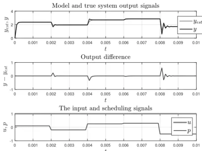
2.5 Output difference between frozen-equivalent LPV models for a switching p . . . . 29
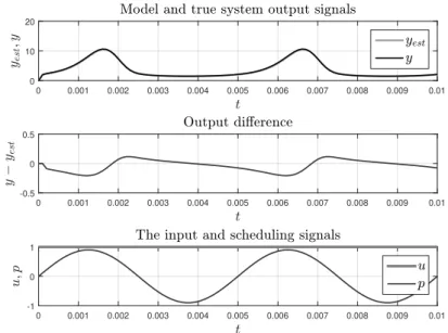
2.6 Output difference between frozen-equivalent LPV models for a sinusoidal p . . . 30
2.7 Interconnection between an LFR with a controller . . . 31
2.8 Interconnection between an LFR with a controller and the uncertainity matrix . . 32
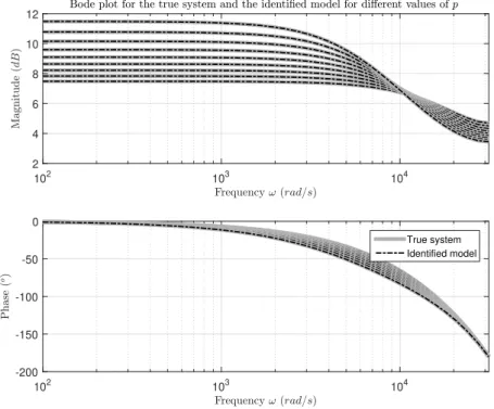
4.1 Bode plot for the true system and identified models for several values of p . . . . 75
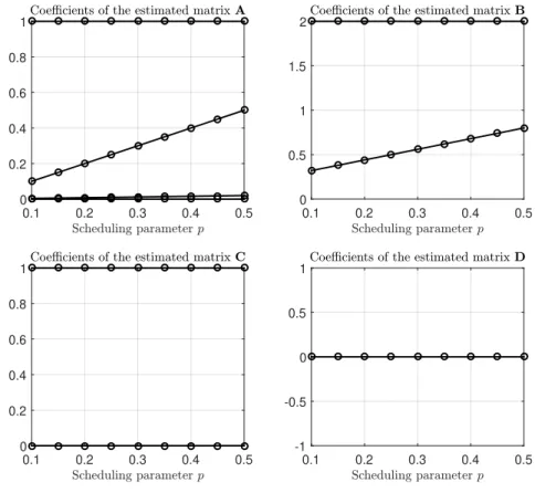
4.2 Evolution of the parameters of the obtained matrices w.r.t p . . . 76
4.3 Output difference vs. scheduling signal frequency . . . 77
4.4 The modeling error and error bound a varying p . . . 78
4.5 The modeling error and error bound aother varying p . . . 79
4.6 The modeling error and error bounds a switching p . . . 80
4.7 The modeling error and error bound for one switching interval of p . . . 81
4.8 Required time to reach a certain error . . . 81
Introduction
M
Athematical models are used to describe real word phenomena using math-ematical equations. Models can have different goals like explaining phys-ical phenomena, making predictions of their behavior or for controller synthesis. In the latter case, the goal is to restrict their behavior to a desired part. Mathe-matical models are used in technical fields like mechanical, communications and geophysical engineering for various applications like signal processing, fault de-tection, pattern recognition and many other purposes. Moreover, models are used in the less-technical sciences like biology, for obtaining more knowledge on the studied objects. Physical phenomena are usually called "dynamical systems" or simply "systems" in the control and systems engineering. Dynamical systems can be subject to external variables, known as inputs. The observable variables of a sys-tem are usually called outputs. Hence, an important goal of a model is to describe the relationship between the inputs and the outputs, i.e., input-output relationship (behavior)of the given system.There exist two major approaches to obtain a dynamical model that describes a certain process [Ljung 1999,Söderström 1989]. The first one is based on deriving differential equations of the system from the basic physical principles. This leads to what we call a white-box model in the case where all values of the system param-eters are known a priori, and to a gray-box when at least one value of the paramparam-eters is unknown. The unknown values thus should be obtained experimentally. The second approach is based on fitting system input-output measurements to a gen-eral model structure with unknown parameters, that do not correspond directly to physical attributes of the system. This approach is called black-box modeling. Both gray-box and black-box models are used in system identification literature. Based on data availability and current computational power that allows for differ-ent simulation scenarios in a relatively short time, black-box models are gaining more space in system modeling area [Ljung 1999,Söderström 1989]. Moreover, de-riving gray-box models for complex systems is tedious and can be sometimes even unfeasible, however, they are more intuitive and trust-worthy than black-box ones, specially when we have an idea of what the values of the real parameters should be.
In many cases the model itself is an artifact, and only the relationship between the inputs and the outputs is of interest to the end user. That is why all models that describe the same real system should be input-output equivalent, i.e., they should result in the same output for any input applied to these equivalent models. System identification handles the question of building mathematical models of dynamical systems based on measured data, where the resulting models should have a similar input-output behavior to that of the true system. Moreover, the
sub-discipline of control theory which deals with the relationship between the input-output behavior of a give system and the properties of the selected model is called realization theory. In this thesis, we focus on theoretical issues related to system
identification and realization theory.
Different classes of mathematical models have been investigated for several years. In the recent history, the simplicity of a system model was crucial to its use-fulness. The complicated systems with non-linearities in their governing equations were usually approximated by linear ones. This approximation had a great suc-cess [Ljung 1999,Söderström 1989], and the theory of Linear Time-Invariant (LTI) systems had a great impact on the industry [Kailath 1980,Rugh 1996,Dorf 2008]. The main reason behind this success is due to its simplicity: the LTI framework contains a huge number of tools that allows both the modeling process and the control of the system to be carried out in a well established theory.
Input✲ LTI System Output✲
Figure 1.1:General LTI system
The situation has changed in the past few decades [Apkarian 1995, Sename 2013, Briat 2015, Isidori 1995, Zhou 1996], and the increasing computa-tional power of computers allows the use of more complicated models that better describe the given system. More complicated models help to fulfill the increasing demands for better performance from the end user. One class of such models which started gaining attention in the past few decades is the class of Linear Parameter-Varying (LPV) models [Shamma 1993, Tóth 2010, Lopes dos Santos 2011,Sename 2013]. LPV models are sometimes viewed as a col-lection of LTI models, whose parameters vary with time. More precisely, the model can depend in a non-linear way on time-varying signals which are usually called the scheduling signals, and denoted by p(t) in Fig.1.2, compared to the LTI case in Fig.1.1, where the only external signals are the inputs and the outputs, and the sys-tem itself is time-invariant. The idea behind the LPV models is seductive because they are close to the LTI ones, and yet can handle a wide class of non-linearities of real world systems. Examples of such varying parameters could be the altitude of an airplane [Marcos 2004], the angle of a robotic arm [Vizer 2015b], the mass and moment of inertia of a flying launcher [Marcos 2015] or the speed of the wind for aerodynamic applications [van Wingerden 2008, van Wingerden 2010]. All these mentioned quantities change over time during operation, and the world is full of such examples.
Input✲ LPV System Output✲
✇
p(t)
Figure 1.2: General LPV system
Although, the control theory of LPV systems is relatively well established [Lee 1997a,Balas 2002,Mohammadpour 2012,Sename 2013], methods for obtain-ing accurate LPV models which describe the real systems in a satisfyobtain-ing way are still a subject of ongoing research and far from being complete. A lot of work is still needed in order to bring LPV system identification to practical use like the LTI case. This manuscript tries to fill some of the existing gaps in the LPV systems
identification theory.
In the following section, we give a deeper look on system identification.
1.1 System identification
Roughly speaking, system identification is the science that tries to solve the fol-lowing problem
“ Given a dynamical system, find a model that describes its input-output be-havior the best”
To solve the identification problem, it is usually broken out to four major steps as follows (modified from [Ljung 1999,Tóth 2010]):
Step 1: Experiment design, data collection and manipulation. Step 2: Model class and structure selection.
Step 3: Estimation of a model with respect to a chosen criterion. Step 4: Model validation.
While all steps are inter-dependent, we give a brief overview of each individual step.
Step 1: Experiment design and data collection
The first step consists in performing experiments on the real system and ob-taining input-output measurements. In this step, the user normally should focus on choosing the best input signal that excites the system the best
according to user defined criteria, and thus results in input-output data sets that contain maximum information about the system [Söderström 1989, Ljung 1999,Khalate 2009].
Step 2: Model class and structure selection
It does not matter how exciting the input is, or which identification algorithm we choose, we cannot obtain a good approximation of the true system unless we select an appropriate model structure. This step is considered to be the most crucial one in the identification process [Ljung 1999, Tóth 2010]. The model structure describes how the inputs and the outputs of the system are related to each other. The user faces several problems during the model selec-tion step. One problem is determining the dimension of the model, which re-flects, roughly speaking, the number of model parameters. Another problem that the user should solve is determining the existence of unique parameter values of the selected model structure that corresponds to the given input-output behavior. This problem is called the identifiability of the model struc-ture. In other words, trying to determine the "true" values of the parameters of non-identifiable model through system identification is not a well-posed problem, because there is no unique solution to the identification problem [Bellman 1970]. Moreover, the problem of verifying whether the obtained data set allows us to distinguish between two models that belong to the se-lected model class is usually called Informativity of the data set, and the cor-responding input is called adequately exciting input [Ljung 1999, Tóth 2010]. Notice that informativity is related to both the model structure and the exper-imental data. This means that the user might have to perform different ex-periments for different model structures, and thus Step 2 can be interchanged with Step 1.
Step 3: Estimation of the unknown parameters of the model
In order to estimate the model parameters, one should choose an optimiza-tion criterion. This criterion can be, for example, a mean squared error be-tween the real outputs and the predicted ones of the model. Then, an opti-mization algorithm is chosen to optimize the selected model parameters to satisfy the criterion [Söderström 1989,Ljung 1999,Tóth 2010]. Actually, this step is the most addressed one between all identification cycle steps, and dif-ferent methods exist for estimating the parameters of LTI and LPV models.
Step 4: Validation of the obtained model
Model validation means accepting the obtained model as a "good descrip-tion" of some aspects of the real system. The choice of the optimization criterion and the validation method can affect the validation result. Prior information about the real system and cross validation can greatly help in
determining whether the model is "close enough" to the real system or not [Söderström 1989,Ljung 1999].
While we still face challenges in all steps of the identification of LPV models, we mainly focus in this work on the problems related to model selection and its possi-ble effect on other steps of the identification process of a given system, and control design for the obtained model.
In the next section, we present some of the used model structures for realizing LPV models. In addition, we provide more details about the main existing gaps in the theory of LPV system identification that we are trying to fill: identifiability analysis of the selected model structure, the equivalence between different model structures, and the relationship between different models obtained using different identification techniques.
1.2 Motivation and contributions
Several challenges in system identification literature of LPV systems are some-times overlooked or just did not have the chance to be faced yet. While there is a lot of focus on developing identification algorithms that handle LPV models structures, the problems in model structure selection has not gained enough attention so far. In this manuscript, we focus on the problems related to model structure selection, and their possible effects on other steps in the identification cycle. LPV models can be represented using different model classes [Tóth 2010]. Input-output models are, arguably, the most famous ones in system identification. Roughly speaking, an input-output model is a di-rect relationship between the input of the system and the measured output of the system. This relationship is realized using several coefficients that weigh the effect of past input and output values on the current value of the output in one simple equation, which is suitable for describing Input Single-Output (SISO) systems. However, other important model representations are State-Space Representation (SSR) and Linear Fractional Representation (LFR) [Tóth 2010, Lee 1996] which are more suitable for describing Input Multi-Output (MIMO) systems. These two representations are very close to each other, and both contain additional variables beside the input and the output of the system. These variables are usually called state variables [Rugh 1996], and they are usually internal variables in the model and might correspond to physical components of the real system. However, state variables might not be directly measured. State-space models are widely used for both identification and control [Apkarian 1995, Biannic 1999, van Wingerden 2007, van Wingerden 2009]. The main different between SSR and LFR is that in the LFR settings, we can usually sep-arate away the uncertainties of the system, in addition to time-varying parameters to a separate block from the time-invariant part of the system. This property gives a strong advantage for designing robust controllers for system with uncertainties or with time-varying parameters. LFR has been widely used in control synthesis of LPV systems or for H∞and optimal control [Zhou 1996,Rugh 2000,Briat 2015].
More recently, the LFRs have attracted a lot of attention as far as system identifica-tion is concerned [Lee 1996,Lee 1997b,Lee 1999,Casella 2008,Vizer 2013c]. Based on above discussion, in this thesis, we will study LPV models in both SSR and
LFR and we will study the relationship between them as follows.
A basic question which one should ask after choosing a model structure is whether this structure is identifiable from the input-output measurements or not. Since LPV models can be seen as a collection of LTI models, it is very common, instead of performing system identification for the LPV model itself, to try to identify a set of LTI models and then try to recover the original LPV models using interpolation methods [Lovera 2007b, Tóth 2010, Zhang 2015,Vizer 2013a]. This is done usually by selecting several constant scheduling signals, which will result in several LTI models. This approach is a very promising one. However, certain issues related to this technique of identification of LPV models still need to be solved. First, if one is interested in structured models, e.g., gray-box models, identifiability analysis is needed in order to guarantee the existence of a unique solution for the identification problem. More precisely, if we are given a certain LPV model with a certain structure, there is no guarantee that by using a constant scheduling signal it is possible to recover all unknown parameters or the LPV model based on the identified LTI ones. This is due to the fact that using constant scheduling signals does not excite the part of the system which is related to the change in scheduling signals. This is actually the main motivation behind performing global identification techniques for LPV system, i.e., using a varying scheduling signal during the identification experiment. This means that the identifiability analysis of LPV models, cannot be performed using already existing tools for LTI ones. That is mainly why we will devote the first part of this thesis
to studying the identifiability of LPV models, where we provide new tools for verifying identifiability of state-space LPV models.
As mentioned above, LPV models can be identified using local identification techniques. However, since LTI models describe only the behavior of the system for constant scheduling signals, we are not sure that the resulting LPV model will describe the system very well in the case of changing scheduling signals. That is
why we will try, in the second part of this thesis, to characterize the resulting modeling error, when such approach for LPV system identification is chosen.
Finally, the equivalence between different model structures which are used for modeling LPV systems is studied. Motivated by the use of LFR for control design, and SSR for model identification, we study the transformation of a model represented in one framework to the other. This conversion is partially known and already used in the literature [Verdult 2002a,Vizer 2013a], but the expressive power of the two model classes and possible preservation of structural properties were not studied yet. For example, we do not know if any model which belongs to one class can be obtained by converting a model from the other class. We also do not know whether this transformation preserves important structural properties like minimality and identifiability. Indeed, it is of prime interest to characterize
the relationship between SSR and LFR for LPV systems in order to be able to manipulate input-output equivalent models in different model classes, which is done in the last part of this thesis.
1.3 Outline of the thesis
In this section, we present the outline of the manuscript and give a brief presenta-tion of the content of each chapter.
Chapter2
In this chapter, several theoretical challenges in system identification of LPV sys-tems are pointed out. This is done by presenting an overview of current LPV system identification techniques. Moreover, basic definitions of LPV systems are provided for both state-space and linear fractional representations. We show that structural properties of LPV systems play an important role in obtaining consistent results in system identification. That is why, we present several examples to show the relationship between structural properties of LPV systems in different repre-sentations and possible shortcoming of state-of-the-art identification techniques. Chapter3
In this chapter, we handle our first challenge, which is the identifiability of LPV state-space models with affine dependence on the scheduling parameters. A new sufficient and necessary condition is introduced in order to guarantee the struc-tural identifiability for ALPV parameterizations. In addition, we present a suf-ficient and necessary condition for local structural identifiability, and a sufsuf-ficient condition for (global) structural identifiability which are both based on the rank of a user-defined matrix. These latter conditions allow systematic verification of identifiability. The results of this chapter are published in [Alkhoury 2017b]. Chapter4
In Chapter4, we study the systematic modeling error of the local approach in LPV system identification. We give an analytical expression for an upper bound on the difference between any two different LPV models, that have the same behavior for constant scheduling signals. Actually, one of these two models can be considered to be the true system, and the other is the result of the local identification method. The given expression for the bound on what can be seen as systematic error of LPV local identification technique allows for better understanding of the influence of different parameters on the modeling error, and can be of great help for controller design when we have a rough understanding of the behavior of the system. The results of this chapter are published in [Alkhoury 2017a].
Chapter5
In this chapter, we study the transformation from Affine Linear Parameter-Varying (ALPV) state-space representation into Linear Fractional Representation (LFR) and vice versa. More precisely, we pay attention to structural properties like minimality, input-output behavior and identifiability of LPV models in both representations. We then characterize LFRs which correspond to equivalent ALPV models based on their input-output maps. As illustrated all along the chapter, these results have im-portant consequences for identification and control of systems described by LFR. The results of this chapter are published in [Alkhoury 2016].
Chapter6
In this chapter, we sum up all obtained results and give our view regarding possi-ble future work to follow the one provided in this manuscript.
1.4 Publications
The work done in this thesis has led to the following publications. Journal papers [1]
1. [Alkhoury 2017b] Ziad Alkhoury, Mihály Petreczky, Guillaume Mercère, Identifiability of Affine Linear Parameter-Varying models, Automatica, (80), pages 62 - 74, 2017.
Conference proceedings [2]
1. [Alkhoury 2017a] Ziad Alkhoury, Mihály Petreczky, Guillaume Mercère, Comparing global input-output behavior of frozen-equivalent LPV state-space models, Proceedings of IFAC 2017 World Congress, Toulouse, France. 2. [Alkhoury 2016] Ziad Alkhoury, Mihály Petreczky, Guillaume Mercère,
Structural properties of affine LPV to LFR transformation: minimality, input-output behavior and identifiability, Proceedings of Decision and Control (CDC), 2016 IEEE 55th Conference on, 3781-3786, Las Vegas, USA.
Background and problem
formulation
2.1 Introduction
Linear parameter-varying (LPV) models are a special class of nonlinear models. They can be seen as an extension of Linear Time-Invariant (LTI) representations where the model parameters are functions of measurable time-varying signals, which are usually called the scheduling signals [Shamma 2012,Wood 1996].
LPV models are widely used in the literature, to name a few ap-plications: aerospace [Doll 2008], [Marcos 2004, Marcos 2008], [Lu 2006], [Lee 2001], [Pfifer 2015], [Hecker 2014], automotive [Novara 2011], [Wei 2006],
mechatronic systems [Giarré 2006], [Steinbuch 2003], [Paijmans 2006] and [Ruiz 2012], wind turbines [van Wingerden 2008], aeroelastic flutters
[van Wingerden 2010], freeway traffic [Luspay 2011], robotics [Vizer 2015a], [van Helvoort 2004], [Abbas 2011], [Mercère 2011a], [Hashemi 2012],
thermody-namics [Mercère 2011b], web systems [Qin 2007], [Tanelli 2008].
While control theory for LPV systems is rather complete [Lee 1997a, Mohammadpour 2012, Balas 2002, Sename 2013], there are still a lot of open problems in system identification of LPV systems. There seems to be a wide range of LPV system identification methods and concepts under ongoing re-search, including, regression approaches [Bamieh 2002], [Hsu 2008], [Tóth 2008], [Tóth 2009], [Tóth 2011a], subspace techniques [Nemani 1995], [Lovera 2007b], [van Wingerden 2007], [van Wingerden 2008], [van Wingerden 2009], [Verdult 2002a], [Verdult 2002b], [Verdult 2004], [Verdult 2005], linear matrix
inequalities based techniques [Mazzaro 2001], nonlinear programming based
methods [Lee 1999], set-membership approach [Cerone 2008], successive
ap-proximation based algorithms [Lopes Dos Santos 2008], Bayesian approach [Golabi 2014], [Darwish 2015], [Golabi 2017]. The variety of these methods seems to be promising. Indeed, there is a great focus on algorithmic and numeric proper-ties of state-of-the-art identification methods, however, their formal mathematical analysis remains challenging. Indeed, as already mentioned in [Tóth 2010], there is still a need to bring all LPV system identification to a common ground, and many gaps in system theory for identification still need to be filled. In particular, there are several basic theoretical questions which remain open.
Informally, as it was already briefly mentioned in section 1.1, the thesis ad-dresses the following issues:
1. Identifiability analysis: we provide conditions that allow us to verify the identifiability of Affine LPV models.
2. Equivalence between different model classes: we study the relationship between various LPV models, in particular SSR and LFR models.
3. Systematic modeling error: we characterize the systematic error resulting while identifying LPV models from a set of experiments for several constant scheduling signals.
These issues relate to system identification as follows. Recall the steps of system identification cycle presented in section 1.1. Then, the relationship between the above mentioned issues and the steps of system identification cycle is explained below:
Identifiability analysis The problem of identifiability analysis of LPV models
can be considered as a problem of model selection. Actually, identifiability analysis is one of the main missing ingredients in LPV system identification. In addition to telling us whether there is a unique solution for the identification problem or not, it helps in analyzing the performance of LPV identification methods. In section2.4.1, we will show that identifiability of LPV models cannot always be studied using tools dedicated to LTI models. That is mainly why we need new tools to verify identifiability of LPV models.
Equivalence between different model classes The relationship between
differ-ent LPV model classes is also a problem of model selection. LPV models are rep-resented using different model classes for different purposes like identification and control. For instance, the Linear Fractional Transformation (LFT) is one of the main tools used in the past decades for studying uncertain systems (see, e.g., [Zhou 1996]). LFT is the tool to obtain Linear Fractional Representations (LFRs), which have been widely used in control synthesis of LPV systems or for H∞
op-timal control (see [Zhou 1996, Rugh 2000, Briat 2015] for an overview). More re-cently, the LFRs have attracted a lot of attention as far as system identification is concerned, (see [Lee 1996,Casella 2008,Vizer 2013c]). For LPV model-based con-troller design, several solutions include transforming the LPV system into an LFR. This step indeed allows us to use control tools developed for LFR models to design a controller to guarantee the satisfactory closed loop operation of the LPV plant in many operating conditions. As far as system identification is concerned, it is clear from the literature (see, among others, [Tóth 2010,Lovera 2014]) that the branch of data-driven modeling dedicated to LPV State-Space model identification is a lot more mature than the one dealing directly with LFR. These observations mean that, in control design as well as in system identification, LPV state-space mod-els are often used as an intermediary representation, whose main purpose is to serve as a source for an LFT description. We already know that an LPV model in SSR can be converted to another one in LFR and vice versa. However, we do not know what happens to structural properties of these model during the conversion. In section2.4.3, we will show possible issues that can be caused when structural properties are not preserved during the transformation from one representation to the other.
Systematic modeling error Identification of LPV models from a set of
experi-ments for several constant scheduling signal is related to both experiment design and model selection. This approach (which is called the local approach) is actually very common and many local approach algorithms have been recently developed. However, we will show in section2.4.2that, in general, it is not possible to recover the whole LPV model using such kind of experiments, no matter how "well" we choose the operating points (the constant values of the scheduling signals). Thus, we will characterize the modeling error which results from such identification approach.
In this thesis, we try to focus on the afore mentioned issues. Solving these problems will, in the long term, help us to obtain satisfactory results in LPV sys-tem identification and control, and to analyze formally the performance of identi-fication algorithms. In order to explain in details the nature of these problems and their solutions, we need to present a number of formal definitions. The goal of this chapter is to accomplish this task, that is, to present a rigorous problem formula-tion and to present the necessary background material on realizaformula-tion theory and systems identification of LPV models.
Realization theory deals with the relationship between the behavior of the sys-tem and the properties of the selected model. Several problems are studied within realization theory. We are interested in realization theory, because it allows us to characterize identifiability and equivalence of state-space representations. Re-alization theory for general LPV systems with meromorphic dependence on the scheduling parameters was developed in [Tóth 2010]. Certain aspects of realiza-tion theory for LPV systems with affine dependence on the scheduling parameters were studied in [Tóth 2012,Verdult 2002a]. A more complete theory is presented in [Petreczky 2012] and [Petreczky 2016]. Combining [Tóth 2010], [Petreczky 2012] and [Petreczky 2016] forms a relatively complete and constructive theory. More precisely, in [Petreczky 2012, Petreczky 2016], conditions are presented to show when certain input-output map admits an LPV realization with affine dependence on the scheduling parameters.
Although well known, we see that it is mandatory to start with the basic definitions and notions of Linear Time-Invariant (LTI) systems. The reason behind this is twofold. On the one hand, LPV systems are sometimes seen as a set of LTI systems, where LTI system theory is used directly. On the other hand, LPV systems can be handled as an extension of LTI systems, where many definitions of LTI systems are extended to LPV systems as we will show later in the chapter.
In this thesis, we will study discrete-time MIMO systems. Focusing on the discrete-time case is chosen for the sake of simplicity and because discrete-time systems are more prominent in system identification. We conjecture that many of the presented results could be extended to the continuous-time case, but the details of such an extension remain a topic of future research.
Outline: In section 2.2 we present main definitions for LTI models in state-space representation. Then, in section2.3, we present different representations of
LPV systems that will be used all along this manuscript. Later in section 2.4, we present the theoretical challenges in system identification that we will study in the next chapters. Finally, in section2.5, we present the conclusion of this chapter.
2.2 State-space representation of LTI systems
To present the formal definitions, we will need the following notation.
Notation1. In the sequel, we assume that ny, nu, nx ∈ N, where N denotes the set
of all natural numbers. Let t denote the discrete-time instant, i.e., t ∈ N as well. Moreover, we denote by Ij
i the set{i, i + 1, . . . , j − 1, j}, where i, j ∈ N, j > i. The
n× n identity matrix will be denoted by In. When its dimension is clear from the
context, the identity matrix will be denoted simply by I. The set of real numbers is denoted by R and the set of complex numbers is denoted by C. We denote by GL(n) the set of n × n invertible matrices, whose entries are in R.
Definition 1 (LTI state-space models [Kailath 1980]). A discrete-time Linear Time-Invariant (LTI) state-space model▲ is defined as follows
▲{ xy(t)(t + 1) = ❆x(t) + ❇u(t),= ❈x(t) + ❉u(t), (2.1) where x(t) ∈ X = Rnxis the state vector at time t, y(t) ∈ Y = Rnyis the output vector
at time t, u(t) ∈ U = Rnu is the input vector at time t, and ❆∈ Rnx×nx,❇ ∈ Rnx×nu,
❈∈ Rny×nxand❉∈ Rny×nu. In the sequel, we will use the notation
▲= (nx, nu, ny,❆, ❇, ❈, ❉) (2.2)
for an LTI model of the form (2.1). The dimensions nx, nu and nywill be dropped
out of the definition when they are clear from the context.
Now, we will define what we mean by dimension of an LTI model.
Definition 2 (Dimension of an LTI model [Kailath 1980]). The dimension of an LTI model▲ denoted by dim(▲) is the dimension nxof its state-space.
The input-output relation of an LTI system, which is described using a state-space representation, can be uniquely determined by the so-called Transfer Func-tion (TF) [Kailath 1980]. We will denote the input-output relation usually by Y , and the input-output relation or a certain model▲ by Y▲. The Transfer Function
(TF) is defined next.
Definition 3 (Transfer Function (TF) [Kailath 1980]). The transfer function❍▲(③)
of an LTI model▲ = (❆, ❇, ❈, ❉), which determines the relationship between its inputs and outputs, is defined by the equation
❍▲(③) = ❉ + ❈(③I − ❆)−1❇, (2.3)
when the inverse(③I − ❆)−1is well defined, i.e., when③∈ C is not an eigenvalue of
Definition 4 (Input-output equivalent LTI models). We say that two LTI models
▲1 = (❆1,❇1,❈1) and ▲2 = (❆2,❇2,❈2) are input-output equivalent, or simply
equivalent, if❍▲1(③) = ❍▲2(③), where ③ is not an eigenvalue of either of ❆1 or of
❆2.
Now, we define minimal LTI models.
Definition 5 (Minimal LTI models). Given a linear system▲ with state dimension nx, we say that ▲ = (❆, ❇, ❈, ❉) is minimal, if there is no other linear system ˜▲ =
(˜❆, ˜❇, ˜❈, ˜❉) whose state dimension ˜nx< nx, such that∀③ ∈ C, ❍▲(③) = ❍▲˜(③).
For a given LTI model▲= (❆, ❇, ❈, ❉), it is easy to obtain input-output equiv-alent model ˜▲ using similarity transformations defined below.
Definition 6 (LTI similarity transformation "isomorphism" [Kailath 1980]). A non-singular matrix❚∈ GL(nx) is said to be a similarity transformation, or an
isomor-phism, from▲= (❆, ❇, ❈, ❉) to ˜▲ = (˜❆, ˜❇, ˜❈, ˜❉) if ˜ ❆= ❚❆❚−1, (2.4a) ˜ ❇= ❚❇, (2.4b) ˜ ❈= ❈❚−1, (2.4c) ˜ ❉= ❉. (2.4d)
Moreover, we say the▲ and ˜▲ are isomorphic if they are related by a similarity transformation.
Notice that, in definition6, the two LTI models▲ and ˜▲ have the same transfer function∀③ ∈ C, ❍▲(③) = ❉ + ❈(③I − ❆)−1❇ = ˜❉ + ˜❈(③I − ˜❆)−1❇˜ = ❍˜
▲(③). This
means that the state-space representation of an LTI transfer function is not unique. However, this does not mean that all input-output equivalent models are related by similarity transformation, as shown in the following example.
Example 1. Let us consider the LTI models▲(θ) = (❆(θ), ❇(θ), ❈(θ), 0), such that θ∈ R, and
❆(θ) = [−θ −θ − 1]0 1 , ❇(θ) = [01],
❈(θ) = [θ 1] .
We can easily prove that▲1 = (❆1,❇1,❈1, 0) = ▲(θ = 1) and ▲2 = (❆2,❇2,❈2, 0) =
▲(θ = 2) are input-output equivalent by calculating their transfer functions, i.e., ❍▲1(③) = ❍▲2(③) =
1
Now, we try to find a similarity transformation between these two LTI models. Define
❚= [❚11 ❚12
❚21 ❚22] , (2.6)
To find the similarity transformation between▲1and▲2, we try to solve the
equa-tion ˜❇= ❚❇. We get directly that ❚12= 0 and ❚22= 1. Then, we solve ˜❆❚ = ❚❆, it
give us that❚21= 0 and at the same time ❚21= −1 which is impossible. This means
that there is no solution, i.e., there is no isomorphism between▲1and▲2.
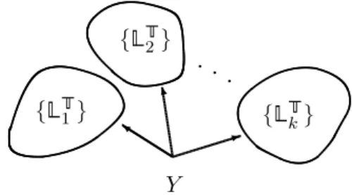
Let us try to represent input-output equivalent models in Fig.2.1. In this figure, we denote by Y a certain input-output relation.▲1,⋯, ▲kare LTI models that have
the same input-output relation Y . We assume that, there is no similarity trans-formation between any two models from the set{▲1,⋯, ▲k}. Now let us denote
by {▲❚i }, i ∈ Ik
1, the set of all models which are isomorphic to the LTI model▲i.
This means that a certain input-output behavior Y can be realized in state-space representation using different sets of LTI models, which do not intersect between each other. This can be an issue in a case when we have a certain input-output re-lation, and we want to search for models which are realizations of this relation. In other words, if we could find one model▲Y that realizes a relation Y , we can
eas-ily characterize all models which are isomorphic to▲Y using the similarity
trans-formations. However, it will be difficult to find other realizations which are not isomorphic to▲Y, which can be an issue if we are interested in identifiability
char-acterization of a certain model structure as we will see later in this manuscript.
{▲❚ 1} {▲❚ 2} {▲❚ k} ❦ ❖ ✶ Y . . .
Figure 2.1:Realizations of an input-output map Y . Here▲iis a realization of Y , and {▲❚i}denotes
the set of all realizations of Y that are isomorphic to▲i.
Now we introduce a very important result for LTI models, which is extended for LPV models later in this chapter.
Theorem 1 ( [Kailath 1980]). All minimal LTI model, which have the same transfer func-tion are related by similarity transformafunc-tion. Moreover, there is a unique isomorphism between any two minimal input-output equivalent LTI models.
This theorem tells us that all minimal models, which are input-output equiv-alent can be characterized using similarity transformation. More precisely, there is only one set of minimal dimension LTI models which realizes a certain input-output behavior. This property is illustrated in Fig.2.2, where there is only one
set of minimal models which realize a certain input-output behavior Y . It is also inevitable to mention the importance of this theorem (which will be extended to LPV systems) in system control theory. Minimal models are easier to handle than non-minimal ones mainly for two reasons, computational reasons and conceptual ones. It is obvious that the fewer the dimensions of the system matrices are, the easier the to handle on a computational level. Moreover, this property of minimal models has big impact on system identification and identifiability characteriza-tion, because it allows us to find all minimal realizations of a certain input-output behavior Y using similarity transformations. This property will be discussed in details later in Chapter3.
{▲❚ min}
Y
❃
Figure 2.2: LTI minimal realizations of a map Y , Here▲minis a realization of Y , and {▲❚min}
denotes the set of all minimal realizations of Y (they are all isomorphic to▲min).
We move now to present basic definitions and the current state of Linear Parameter-Varying Systems theory.
2.3 Representations of LPV systems
It is common to use transfer functions to describe the input-output relationship of an LTI model. However, for LPV models, the definition of transfer function no longer holds. This is the main reason why we need new tools for handling and characterizing equivalence of LPV models. There are two main approaches for describing an input-output behavior of an LPV system. The first is called the behavioral approach, which is developed in [Tóth 2010, Tóth 2011b] for LPV sys-tems, and the other uses input-output maps [Petreczky 2012, Petreczky 2016]. In Appendix2.A, we explain how these two approaches are related to each other.
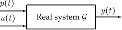
u(t) ✲ Real systemG y(t)✲
✲
p(t)
Figure 2.3: Real system that we want to describe using an LPV model
In this manuscript, we will use input-output maps to describe a real systemG, illustrated in Fig.2.3, where u(t) represents the inputs of the system at time t, p(t)
is the scheduling signals at time t and y(t) is the outputs at time t. An input-output mapF can be defined as follows:
F ∶ U × P → Y, (2.7)
where U, P, Y are the input, the scheduling and the output signals spaces respec-tively. The value of F(u, p)(t) represents the outputs of the system G at time t, considering that u and p are fed to the system. Note that this value depends on all the values of u and p from the initial time instant t0 until the time instant t. In
other words, we can write
y(t) = F(u, p)(t). (2.8)
Input-output maps can be realized using different models. The most known ones are the Input-Output Representation (IOR), the State-Space Representation (SSR) and the Linear Fractional Representation (LFR) [Ljung 1999, Zhou 1996]. While both IOR and SSR are very common in system identification [Ljung 1999], the LFR is very important for control synthesis [Zhou 1996]. In this thesis, we will use SSR and LFR to describe LPV models, i.e., to realize input-output maps of LPV models and study the relationship between them.
Now, we will present formal definitions that will be used in this thesis. Let us start with defining LPV models in SSR.
2.3.1 State-space representation of LPV systems
Definition 7 (Discrete-Time LPV State-Space (DT-LPV-SS) models). A
discrete-time Linear Parameter Varying state-space model Σ is defined as follows Σ⎧⎪⎪⎪⎨ ⎪ ⎪ ⎪ ⎩ x(t+ 1) = A(p(t))x(t) + B(p(t))u(t), y(t) = C(p(t))x(t) + D(p(t))u(t), (2.9) where x(t)∈ X = Rnxis the state vector at time t, y(t)∈ Y = Rnyis the output vector
at time t, u(t)∈ U = Rnuis the input vector at t and p(t)∈ P ⊆ Rnp is the scheduling
signal vector at time t. The matrix functions A ∶ P ↦ Rnx×nx, B ∶ P ↦ Rnx×nu,
C ∶ P ↦ Rny×nx and D ∶ P ↦ Rny×nu are assumed to be continuous maps. In the
sequel, we will use the short notation
Σ= (P, nx, nu, ny, A(.), B(.), C(.), D(.)) (2.10)
to denote a model of the form (2.9). Notice that we use the notation A(.), B(.), C(.) and D(.) to emphasize that these matrices are maps, not constant matrices. Note that we will drop some or all of the dimensions nx, nu, ny from the definition
and/or the scheduling parameter set P when it is clear from the context.
Remark1 (p is a free signal). In this manuscript, we deal with true LPV systems.
This means that the scheduling signal p does not necessarily depend on the system like in the quasi-LPV systems [Tóth 2010]. In other words, we assume that p is a
free variable with respect to the studied system, i.e., p is an external signal which is fully measurable. Note that the definition of the input-output map in Eq. (2.7) implicitly implies that we are looking at true LPV and not quasi-LPV systems, because we assume that every output signal corresponds to a choice of some input and scheduling signals. Otherwise, it would have been that every output and scheduling signals correspond to a choice of the input signal.
To continue with the definitions, we need the following notation.
Notation2. In the sequel, For a set A, we denote by ANthe set of all functions of
the form φ∶ N → A. An element of ANcan be just thought of as an infinite sequence
or as a signal in discrete-time.
By a solution of Σ we mean a tuple of trajectories (x, y, u, p) ∈ (X , Y, U, P) satisfying Eq. (2.9) for all k ∈ N. Here X = XN
,Y = YN
,U = UN
,P = PN. In other
words P is the scheduling parameter space, U is the input space, Y is the input space and X is the state space. Note that P denotes the set of scheduling signals, while P denotes the set of all possible values of the scheduling parameters. That is, an element of P is a sequence, while an element of P is a vector. The same remark holds for X , Y, U and X, Y, U. Note that in the sequel, unless stated otherwise, we will use p to denote a scheduling signal, and we use p to denote a potential value of the scheduling variable, i.e., p∈ P is a sequence, but p ∈ P is a vector.
Now, we will define what we mean by dimension of an LPV model.
Definition 8 (Dimension of an LPV model). The dimension of an LPV model Σ
denoted by dim(Σ) is the dimension nxof its state-space. Note that the dimension
nxof the model does not depend on the dimension of the scheduling variables np.
Remark2. We assume, all along this thesis, that the state-space matrices depend
on the scheduling signal in a static way, i.e., they depend only on p(t) and not on time-shifted versions like p(t − 1), ⋯, etc.
Next, we define the notion of input-output maps and input-to-state maps of Σ induced by an initial state.
Definition 9 (Input-output map of an LPV model Σ). Let x0 ∈ Rnx be an initial
state of Σ. Define the function
YΣ,x0 ∶ U × P → Y, (2.11)
such that for any(x, y, u, p) ∈ X × Y × U × P, and y = YΣ,xo(u, p) holds if and only if
(x, y, u, p) satisfy (2.9) and x(0) = x0. The function YΣ,x0 is called the input-output
functionof Σ induced by x0.
In the sequel, for the sake of simplicity, we will assume that the initial state is zero. The results of the paper can easily be extended to the case of nonzero initial state. Similarly, we will refer to the input-output map YΣ,0 induced by the initial state
x0= 0 as the input-output map of Σ, and we will denote YΣ,0by YΣ.
Definition 10 (Input-output equivalent LPV models). Two LPV models Σ1and Σ2
Now, similarly to LTI models, we define minimal LPV models.
Definition 11 (Minimal LPV models). Given an LPV models Σ with state
dimen-sion nx. We say that Σ is minimal, if there is no other LPV model ˜Σwhose state
dimension ˜nx< nx, such that YΣ= YΣ˜.
From the discussion above, it follows that the external behavior of an LPV model can be modeled by input-output maps of the form
f ∶ U × P → Y. (2.12)
That is, a function f of the form (2.12) can be viewed as an input-output map of a system which takes control inputs u ∈ U and scheduling parameters p ∈ P as inputs, and responds to them by generating an output trajectory y ∈ Y. Next, we define when an LPV model describes (realizes) f, i.e., when it is true that f describes the behavior of an LPV model. The LPV model Σ of the form (3.1) is a realizationof an input-output map f of the form (2.12) if f equals the input-output map of Σ which corresponds to the zero initial state, i.e., f = YΣ,0. For the purposes
of this manuscript, LPV realizations with the smallest possible number of states will be of interest. Let f be an input-output map. An LPV model Σ is a minimal realization of f, if Σ is a realization of f and, for any LPV model ¯Σ which is a realization of f, dim Σ≤ dim ¯Σ. We say that an LPV model Σ is minimal, if Σ is a minimal realization of its own input-output map YΣ.
A special case of LPV models, i.e., when the state-space matrices are affine func-tion of the scheduling parameter will be of great interest in this thesis. The main reasons for our interest are i) their ability to model a wide range of nonlinearities as will be shown in the section 2.3.2, ii) the relative ease of control synthesis for this class of LPV models [Mohammadpour 2012,Hoffmann 2016], iii) the fact that it already has a Kalman-like realization theory [Petreczky 2012,Petreczky 2016].
2.3.2 State-space representation with affine dependence of LPV systems We present formal definition of Discrete-Time Affine Linear Parameter-Varying State-Space (DT-ALPV-SS) models and their main properties that we will use all along this manuscript. For simplicity, we will use the term "ALPV models" instead of "DT-ALPV-SS models".
Definition 12 (ALPV models). A discrete-time Affine Linear Parameter-Varying
(ALPV) model(Σ) is a discrete-time state-space representation of the form (2.9), where the matrix functions A ∶ P → Rnx×nx, B ∶ P → Rnx×nu, C∶ P → Rny×nx and
D∶ P → Rny×nudefining the LPV model (2.9) are considered to be affine functions,
such that for all p= [p1, p2, . . . , pnp] ⊺∈ P ⊆ Rnp, A(p)= A0+ np ∑ i=1 Aipi, (2.13a) B(p)= B0+ np ∑ i=1 Bipi, (2.13b) C(p)= C0+ np ∑ i=1 Cipi, (2.13c) D(p)= D0+ np ∑ i=1 Dipi. (2.13d)
In the sequel, we will assume that the affine span of the elements of P yields the whole space Rnp, i.e., P does not belong to a non-trivial hyperplane of Rnp. If this is
not the case, then a lower dimensional space of scheduling variables can be chosen. We will use the short notation
Σ= (P, nx, nu, ny,{Ai, Bi, Ci, Di}ni=0p) (2.14)
to define an ALPV model, whose matrices are of the form (2.13). Note also that we will drop the dimensions nx, nu, nyout of the definition and/or the scheduling
parameter set P when clear from the context.
Remark 3. Notice that the affine dependence on the scheduling parameters can
be extended to affine dependence in linearly independent set of functions of the scheduling parameters . More precisely, assume {ψi(p)}
nψ
i=1 is a linearly
indepen-dent set of functions of p. Then, A(p) can depend in an affine way on ψi(p) i.e.,
A(p)= A0+ ∑nψ
i=1Aiψi(p) (see [Petreczky 2016] for more details).
Remark 4. It is important to note that, in this manuscript, all definitions which
are presented for generic LPV systems are also valid for ALPV ones as well unless new definitions are presented.
Now, similarly to generic LPV models, we define minimal ALPV models.
Definition 13 (Minimal ALPV models). Given an ALPV models Σ with state
di-mension nx. We say that Σ is minimal, if there is no other ALPV model ˜Σwhose
state dimension ˜nx< nx, such that YΣ= YΣ˜.
Minimality of a model means there is no any input-output equivalent model that has a smaller dimension. Minimization is the act of converting a model to a minimal one using similarity transformation and allowed truncation. Note that minimization is different from reduction which also results in models with smaller order (dimension). However, the resulting models are not input-output equiva-lent to the original model, but they should have a very close input-output relation [Theis 2016]. Note that model reduction has applications in all aspects of control theory like analysis, controller design and implementation. However, such no-tion is not used in this manuscript. Minimality has a big impact in characterizing equivalent LPV models in a similar way to LTI ones. As far as system identifica-tion is considered, it is intuitive to choose a minimal model to describe the system