HAL Id: hal-00275332
https://hal.archives-ouvertes.fr/hal-00275332
Submitted on 23 Apr 2008
HAL is a multi-disciplinary open access
archive for the deposit and dissemination of
sci-entific research documents, whether they are
pub-lished or not. The documents may come from
teaching and research institutions in France or
abroad, or from public or private research centers.
L’archive ouverte pluridisciplinaire HAL, est
destinée au dépôt et à la diffusion de documents
scientifiques de niveau recherche, publiés ou non,
émanant des établissements d’enseignement et de
recherche français ou étrangers, des laboratoires
publics ou privés.
Video Quality Model based on a spatiotemporal features
extraction for H.264-coded HDTV sequences
Stéphane Péchard, Dominique Barba, Patrick Le Callet
To cite this version:
Stéphane Péchard, Dominique Barba, Patrick Le Callet. Video Quality Model based on a
spatiotem-poral features extraction for H.264-coded HDTV sequences. Picture Coding Symposium, Nov 2007,
Lisbonne, Portugal. pp.1087. �hal-00275332�
VIDEO QUALITY MODEL BASED ON A SPATIO-TEMPORAL FEATURES EXTRACTION
FOR H.264-CODED HDTV SEQUENCES
Stéphane Péchard, Dominique Barba, Patrick Le Callet
Université de Nantes – IRCCyN laboratory – IVC team
Polytech’Nantes, rue Christian Pauc, 44306 Nantes, France
[email protected]
ABSTRACT
As a contribution to the design of an objective quality metric in the specific context of High Definition Television (HDTV), this paper proposes a video quality evaluation model. A spa-tio-temporal segmentation of sequences provide features used with the bitrate to predict the subjective evaluation of the H.264-distorted sequences. In addition, subjective tests have been conducted to provide the mean observer’s quality appre-ciation and assess the model against reality. Existing video quality algorithms have been compared to our model. They are outperformed on every performance criterion.
Index Terms— HDTV, H.264, Subjective quality assess-ment, Modeling
1. INTRODUCTION
Objective video quality metrics are required in order to mon-itor visual quality of sequences for coding purposes or for assessing the visual quality at the user level. Numerous meth-ods already exist working with common video formats like CIF, QCIF or Standard Television (SDTV) [1]. In the last years, High Definition Television (HDTV) began to be broad-casted in few countries. This new technology also requires ef-ficient quality metrics adapted to its specificities. Three types of quality metrics are possible: full reference (FR), reduced reference (RF) and no reference (NR) metrics. To compute a quality evaluation, FR metrics use both original and processed sequences, while RF metrics use a reduced version of the ref-erence and NR metrics only use the processed sequence. In the context of coding purposes (quality measurement and op-timization), FR metrics are the most adapted since both se-quences are available.
Most video quality evaluation methods do not consider coding distortions as a whole, but as individual distortions (blur, blockiness, ringing, etc.) whose effects are combined. Farias’ approach [2] relies on synthetic distorsions applied in-dividually or combined on pre-defined spatial areas of the se-quence. This method is then content-dependent. Wolff [3] uses H.264-distorted sequences. Tasks asked to observers are
first to assess the global annoyance caused by all visible im-pairments on the entire sequence, second to rate the strength of each type of artefact. Subjective evaluation is then compli-cated by the need of isolating distorsions by types, whereas they are mixed in a complex way by the distorting scheme. Moreover, in this HDTV context, one main issue is the com-putation complexity due to the bigger image size.
The proposed model predicts video quality of sequences depending on their coding bitrate and spatio-temporal proper-ties. Such properties are computable offline and depend only on the reference video. Therefore, it is a reduced reference method (RR). The model is intentionally simple in order to produce results as fast as possible. The spatio-temporal fea-tures extraction is a bit more computationally complex but may be done offline. Instead of categorizing distortions, only H.264 coding is considered as a distortion scheme but that can lead to different perceived annoyance depending on the spatio-temporal area where it occurs. The idea is to use a rather simple but efficient spatio-temporal segmentation of the content. This segmentation provide features on spatio-temporal bitrate repartition over the sequence. Such features are used to adjust bitrate-predicted quality of a distorted se-quence. In addition, subjective tests have been realized in order first to obtain a global trend of video quality, then to evaluate the model against reality.
Section 2 of the paper presents the segmentation and clas-sification methodology. Then, section 3 details subjective quality tests conditions and methods. In section 4 the pro-posed video quality model is presented. Then we display and discuss the obtained results before concluding.
2. SPATIO-TEMPORAL SEGMENTATION It is well known that the human visual system (HVS) has a different perception of distortions depending on the local spatio-temporal content of the sequence. Therefore, several content classes have been designed in order to take them into account separately. Three classes have been defined as fol-lows: smooth areas (C1), textured areas (C2) and edges (C3).
spa-Fig. 1. Tube creation process over five frames or fields.
tial activity, consequently with a certain impact of H.264 cod-ing artefacts on the perceived quality. In order to obtain these spatio-temporal zones, a segmentation of the sequence is pro-cessed. Then a classification of each spatio-temporal segment is applied. In the scope of this paper, only the proportions of each class are used. More details on the method are in [4].
2.1. Segmentation
The segmentation process divides the original uncompressed sequence into elementary spatio-temporal volumes. The first part of the segmentation is a block-based motion estimation which enables the evolution of spatial blocks to be tracked over time. This is performed per group of five consecutive frames for progressive HDTV or per groupe of five consecu-tive fields of the same parity (one group of odd and one group of even fields). For each group of five frames or fields, the one i located at the middle is divided into blocks and a mo-tion estimamo-tion of each block is computed simultaneously us-ing the two precedus-ing frames or fields and the two follow-ing frames or fields as shown in Figure 1. As HDTV con-tent processing is of particular complexity, this motion es-timation is performed through a multi-resolution technique. The three-level hierarchical process significantly reduces the computation and provides better estimation. Finally, these temporal tubes are temporally gathered to form spatio-temporal volumes along the entire sequence. This gathering assigns the same label to overlapping tubes as depicted in Fig-ure 2. Some unlabeled ‘holes’ may appear between tubes. They are merged with the closest existing label.
2.2. Tubes merging and classification
The second part of the segmentation is spatial processing. Tubes created by the segmentation are merged based on their positions, enabling objects to be followed over time. This merging step depends on the class assigned to each tube. Each set of merged tubes is classified into a few labeled classes with homogeneous content. The class of a tube is determined from a set of features based on oriented spatial activities computed on it. Depending on these features, a tube may be labeled as corresponding to a smooth area (C1), a textured area (C2) or
Fig. 2. Labeling of overlapping tubes. Sequence k H.264 Bitrates in Mbps (1) Above Marathon 5 ; 8 ; 10 ; 12 ; 16 ; 24 ; 32 (2) Captain 1 ; 3 ; 5 ; 6 ; 8 ; 12 ; 18 (3) Dance in the Woods 3 ; 5 ; 6 ; 8 ; 10 ; 14 ; 18 (4) Duck Fly 4 ; 6 ; 8 ; 12 ; 16 ; 20 ; 32 (5) Fountain Man 1 ; 2 ; 5 ; 8 ; 9 ; 12 ; 20 (6) Group Disorder 2 ; 4 ; 7 ; 8 ; 12 ; 16 ; 20 (7) Inside Marathon 3 ; 4 ; 6 ; 8 ; 10 ; 14 ; 16 (8) New Parkrun 2 ; 4 ; 6 ; 8 ; 10 ; 14 ; 20 (9) Rendezvous 4 ; 6 ; 8 ; 10 ; 14 ; 18 ; 24 (10) Stockholm Travel 1 ; 4 ; 6 ; 8 ; 10 ; 16 ; 20 (11) Tree Pan 1.25 ; 1.5 ; 2 ; 2.5 ; 3 ; 5 ; 8 (12) Ulriksdals 1 ; 2 ; 4 ; 6 ; 8 ; 12 ; 16
Table 1. Set of bitrates (in Mbps) per coded video.
an edge (C3). No information on the edge directions is
con-served. Finally, three labels are used to classify every tube in every sequence. Proportions P1, P2 and P3 of each class in
sequences are presented in Table 2.
3. H.264 CODING AND QUALITY ASSESSMENT A set of H.264-coded sequences are generated from 12 ten-second long original uncompressed 1080i HDTV sequences provided by the swedish television broadcaster SVT. H.264 coding is performed with the H.264 reference software (ver-sion 10.2) as it was in [4]. Seven bitrates are selected in or-der to cover a significant range of quality. Bitrates (in Mbps) used for each sequence are presented in Table 1. All these sequences (original and distorted as well) have been subjec-tively assessed in order to characterize their quality as a func-tion of the coding bitrate. According to internafunc-tional recom-mandations [5] for test conditions, video quality evaluations are performed using the SAMVIQ protocol [6] with at least 15 validated observers, a 1920×1080 HDTV Philips LCD monitor and a Doremi V1-UHD player. Figure 3 shows the obtained rate-MOS curves. MOS stands for Mean Opinion Score, measured on a [0,100] quality scale. One may notice that whereas obtained qualities are of the same range, bitrates have more important variations. This is due to content
0 10 20 30 40 50 60 70 80 90 0 5 10 15 20 25 30 35 MOS Bitrate (Mbps) Above marathon Captain Dance in the woods Duck fly Fountain man Group disorder Inside marathon New parkrun Rendezvous Stockholm travel Tree pan Ulriksdals
Fig. 3. Rate-MOS characterization of the 12 sequences.
ences. Some curves may show a non-monotony with the bi-trate. This is due to some incoherences in the H.264 reference software coding process. Moreover, the obtained intervals of confidence are quite high because of the only 15 people in-volved.
4. VIDEO QUALITY MODEL
From the tests results depicted in Figure 3, a global trend is noticeable. The proposed model gives the video quality V Q, which is a MOS prediction of the sequence k coded at the bitrate Bk, as a function of Bk:
V Q(Bk) = 100 × (1 − exp(−ak× Bk)) (1)
with ak a parameter to be determined for each sequence
k. This parameter is the visual quality factor of a distorted sequence at bitrate Bk due both to bitrate distribution (and
therefore to the proportions of each spatio-temporal class in the whole sequence) and to motion blur perception. The fol-lowing only considers the bitrate distribution effect as motion blur perception is strongly dependent on the display type.
The theoretic limit of 100 is the upper limit of the quality scale. Even if in these tests results, this value is not reached, the model is intend to be used with any type of quality range. This model is a trade-off between simplicity and good corre-lation with tests results. akhas to be predicted and optimized
as close as possible to the nominal parameter. This nominal value is obtained from the rate-MOS characterization step by fitting the model to the obtained quality (MOS):
a′ k= − 1 Bk ln „ 1 −M OS(B100 k) « (2)
with M OS(Bk) the MOS given by observers to the sequence
k at bitrate Bk. Obtained values are given in Table 2.
The spatio-temporal activity distribution in the sequence influences the way the coder shares the allocated bitrate. akis
k P1 P2 P3 a′ (1) 21.2 77.85 0.94 0.045 (2) 91.4 7.17 1.43 0.144 (3) 26.37 70.60 3.02 0.077 (4) 9.10 80.20 10.70 0.045 (5) 81.23 17.30 1.45 0.069 (6) 63.86 34.34 1.79 0.074 (7) 53.28 46.52 0.20 0.082 (8) 74.87 21.16 3.98 0.095 (9) 21.16 76.79 2.05 0.045 (10) 66.65 15.76 17.58 0.107 (11) 18.59 80.72 0.68 0.234 (12) 54.85 43.78 1.36 0.105
Table 2. Nominal values of a obtained by fitting tests results and proportions of each class of every sequence (in %).
therefore predicted using the spatio-temporal classes propor-tions presented in Table 2. Due to their low proporpropor-tions, edges are not considered. We considered that ak can be estimated
by a quadratic functional from P1and P2:
ak(P1, P2) = α1+ α2P1+ α3P2+ α4P 2 1 + α5P
2
2 (3)
where αjare the parameters of the model with j ∈[1, 5] their
index. These were determined by fitting the data to the desired quadratic form in terms of mean squared errors.
5. RESULTS AND INTERPRETATION 5.1. Loss of accuracy due to the a′obtention
An initial indicator of the performances of the model is to compare the 84 MOS obtained from the tests to the predicted ones (MOSp′), using the video quality model with a′values.
Since the model is an approximation of the curves obtained by subjective tests, a loss of accuracy is possible. The linear correlation coefficient (CC) between MOS and MOSp′equals
0.9662. The root mean square error (RMSE) is 5.005. An expected loss of accuracy is present but rather low. More-over, the prediction has very good correlation with the mean observer’s judgment. Therefore, the model may be used to predict the MOS of a coded sequence with parameters a pre-dicted from the classification features.
5.2. Performances of the model
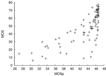
Figure 4 depicts the scatter plot of MOS versus MOSp for all sequences (12) and bitrates (7). CC is equal to0.7374 and RMSE is16.78. The model here is not so good in predict-ing the MOS of these sequences. Actually, two sequences have particularly bad predictions: Above marathon and Ren-dezvous. These two sequences present a high coding com-plexity. The first correspond to a running crowd in the fore-ground with a lot of chaotic movement. The second is a long
0 10 20 30 40 50 60 70 80 26 28 30 32 34 36 38 40 42 44 46 48 MOS MOSp
Fig. 4. MOS versus MOSp for all sequences and bitrates.
pan with several successive plans, creating a sequence diffi-cult to code. Moreover, these two sequences require some of the highest bitrates (up to 32 Mbps) and have amongst lowest a values. In their case, classes proportions are not sufficient to accurately predict a.
The model has been tested without these two specific se-quences. With only ten sequences at seven bitrates for a pre-diction, CC equals0.9062 and RMSE is 7.99. Figure 5 de-picts the new plot. The difference between both results
0 10 20 30 40 50 60 70 80 10 20 30 40 50 60 70 MOS MOSp
Fig. 5. MOS versus MOSp for 10 sequences and all bitrates. its the validity range of the model. It achieves good perfor-mances in a limited range of coding complexity. Two more complex sequences tend to move the prediction away from the mean observer’s assessment. The model is therefore not adapted to such complexity yet. Proportions of classes may be unsufficient information to predict the quality difference between sequences. Other features such as the amount of mo-tion may be used to enhance the model accuracy.
In order to compare the proposed method with existing
Method CC RMSE rank CC VQM 0.8860 9.93 0.8680 VSSIM 0.8799 9.00 0.8549 Proposed 0.9062 7.99 0.8859 Table 3. Comparison with existing approaches.
approaches, the set of 10 sequences has been evaluated by VQM [7] and VSSIM [8] algorithms. Table 3 gives these re-sults in terms of CC, RMSE and Spearman rank coefficient correlation (rank CC). These results are quite high, consid-ering usual performances of these metrics. This is due to the quite uniform content of the 10 sequences. Nevertheless, this comparison shows the slightly higher performances of the proposed method in the limited range of coding complexity.
6. CONCLUSION
This paper proposes a simple video quality model in order to predict the mean observer’s quality judgment. This is done with both the bitrate and the proportions of smooth areas and textures areas of the sequences. The model demonstrated moderate performances on the whole set of sequences but per-formed well against existing algorithms in a limited range of coding complexity, which is the main production in televi-sion.
7. REFERENCES
[1] VQEG, “Final report from the video quality experts group on the validation of objective models of video quality assessment,” Tech. Rep., VQEG, 2003.
[2] Mylène Farias, No-reference and reduced reference video qual-ity metrics: new contributions, Ph.D. thesis, Universqual-ity of Cali-fornia, 2004.
[3] Tobias Wolff, Hsin-Han Ho, John M. Foley, and Sanjit K. Mitra, “H.264 coding artifacts and their relation to perceived annoy-ance,” in European Signal Processing Conference, 2006. [4] Stéphane Péchard, Patrick Le Callet, Mathieu Carnec, and
Do-minique Barba, “A new methodology to estimate the impact of H.264 artefacts on subjective video quality,” in Proceedings of the Third International Workshop on Video Processing and Quality Metrics, VPQM2007, Scottsdale, 2007.
[5] ITU-R BT. 500-11, “Methodology for the subjective assessment of the quality of television pictures,” Tech. Rep., International Telecommunication Union, 2004.
[6] Jean-Louis Blin, “SAMVIQ – Subjective assessment methodol-ogy for video quality,” Tech. Rep. BPN 056, EBU Project Group B/VIM Video in Multimedia, 2003.
[7] Stephen Wolf and Margaret Pinson, “Video quality measure-ment techniques,” Tech. Rep. Report 02-392, 2002.
[8] Zhou Wang, Ligang Lu, and A. C. Bovik, “Video quality as-sessment based on structural distortion measurement,” Signal Processing: Image Communication, vol. 19, pp. 121–132, 2004.