HAL Id: hal-00412264
https://hal.archives-ouvertes.fr/hal-00412264
Submitted on 15 Apr 2020
HAL is a multi-disciplinary open access
archive for the deposit and dissemination of
sci-entific research documents, whether they are
pub-lished or not. The documents may come from
teaching and research institutions in France or
abroad, or from public or private research centers.
L’archive ouverte pluridisciplinaire HAL, est
destinée au dépôt et à la diffusion de documents
scientifiques de niveau recherche, publiés ou non,
émanant des établissements d’enseignement et de
recherche français ou étrangers, des laboratoires
publics ou privés.
An integral approach to causal inference with latent
variables
Sam Maes, Stijn Meganck, Philippe Leray
To cite this version:
Sam Maes, Stijn Meganck, Philippe Leray. An integral approach to causal inference with latent
variables. Russo, F. and Williamson, J. Causality and Probability in the Sciences, London College
Publications, pp.17-41, 2007, Texts In Philosophy series. �hal-00412264�
An integral approach to causal
infer-ence with latent variables.
Sam Maes, Stijn Meganck and Philippe Leray
1
Introduction
This article discusses graphical models that can handle latent variables with-out explicitly modeling them quantitatively. In the uncertainty in artificial intelligence area there exist several paradigms for such problem domains. Two of them are semi-Markovian causal models and maximal ancestral graphs. Applying these techniques to a problem domain consists of sev-eral steps, typically: structure learning from observational and experimental data, parameter learning, probabilistic inference, and, quantitative causal inference.
The main problem is that each of the existing approaches only focuses on one or a few of all the steps involved in the process of modeling a problem including latent variables. The goal of this article is to investigate the integral process from observational and experimental data unto different types of efficient inference.
Semi-Markovian causal models (SMCMs) (Pearl, 2000; Tian and Pearl, 2002a) are an approach developed by Tian and Pearl. They are specifically suited for performing quantitative causal inference in the presence of latent variables. However, at this time no efficient parametrisation of such models is provided and there are no techniques for performing efficient probabilistic inference. Furthermore there are no techniques to learn these models from data issued from observations, experiments or both.
Maximal ancestral graphs (MAGs) (Richardson and Spirtes, 2002) are an approach developed by Richardson and Spirtes. They are specifically suited for structure learning in the presence of latent variables from observational data. However, the techniques only learn up to Markov equivalence and provide no clues on which additional experiments to perform in order to obtain the fully oriented causal graph. See Eberhardt et al. (2005); Meganck et al. (2006) for that type of results for Bayesian networks without latent variables. Furthermore, as of yet no parametrisation for discrete variables is provided for MAGs and no techniques for probabilistic inference have been
developed. There is some work on algorithms for causal inference, but it is restricted to causal inference quantities that are the same for an entire Markov equivalence class of MAGs (Spirtes et al., 2000; Zhang, 2006).
We have chosen to use SMCMs as a final representation in our work, because they are the only formalism that allows to perform causal inference while fully taking into account the influence of latent variables. However, we will combine existing techniques to learn MAGs with newly developed meth-ods to provide an integral approach that uses both observational data and experiments in order to learn fully oriented semi-Markovian causal models. Furthermore, we have developed an alternative representation for the probability distribution represented by a SMCM, together with a para-metrisation for this representation, where the parameters can be learned from data with classical techniques. Finally, we discuss how probabilistic and quantitative causal inference can be performed in these models with the help of the alternative representation and its associated parametrisation.
The next section introduces the necessary notations and definitions. It also discusses the semantical and other differences between SMCMs and MAGs. In section 3, we discuss structure learning for SMCMs. Then we introduce a new representation for SMCMs that can easily be parametrised. We also show how both probabilistic and causal inference can be performed with the help of this new representation.
2
Notations and Definitions
We start this section by introducing notations and defining concepts nec-essary in the rest of this article. We will also clarify the differences and similarities between the semantics of SMCMs and MAGs.
2.1 Notations
In this work uppercase letters are used to represent variables or sets of variables, i.e. V = {V1, . . . , Vn}, while corresponding lowercase letters are used to represent their instantiations, i.e. v1, v2and v is an instantiation of all vi. P (Vi) is used to denote the probability distribution over all possible values of variable Vi, while P (Vi = vi) is used to denote the probability distribution over the instantiation of variable Vi to value vi. Usually, P (vi) is used as an abbreviation of P (Vi= vi).
The operators P a(Vi), Anc(Vi), N e(Vi) denote the observable parents, an-cestors and neighbors respectively of variable Vi in a graph and P a(vi) rep-resents the values of the parents of Vi. Likewise, the operator LP a(Vi) represents the latent parents of variable Vi. If Vi ↔ Vj appears in a graph then we say that they are spouses, i.e. Vi∈ Sp(Vj) and vice versa.
they are dependent by (Vi 2Vj). 2.2 Modeling Latent Variables
First of all, consider the model in Figure 1(a), it is a problem with observable variables V1, . . . , V6 and latent variables L1, L2 and it is represented by a directed acyclic graph (DAG). As this DAG represents the actual problem henceforth we will refer to it as the underlying DAG.
One way to represent such a problem is by using this DAG representation and modeling the latent variables explicitly. Quantities for the observable variables can then be obtained from the data in the usual way. Quantities involving latent variables however will have to be estimated. This involves estimating the cardinality of the latent variables and this process can be difficult and lengthy. One of the techniques to learn models in such a way is the structural EM algorithm (Friedman, 1997).
Another method to take into account latent variables in a model is by representing them implicitly. With that approach, no values have to be estimated for the latent variables, instead their influence is absorbed in the distributions of the observable variables. In this methodology we only keep track of the position of the latent variable in the graph if it would be modeled, without estimating values for it. Both the modeling techniques that we will use in this article belong to that approach, they will be described in the next two sections.
2.3 Semi-Markovian Causal Models
The central graphical modeling representation that we use are the semi-Markovian causal models. They were first used by Pearl (2000), and Tian and Pearl (2002a) have developed causal inference algorithms for them.
Definitions
DEFINITION 1.1. A semi-Markovian causal model (SMCM) is an acyclic causal graph G with both directed and bi-directed edges. The nodes in the graph represent observable variables V = {V1, . . . , Vn} and the bi-directed edges implicitly represent latent variables L = {L1, . . . , Ln′}.
See Figure 1(b) for an example SMCM representing the underlying DAG in (a).
The fact that a bi-directed edge represents a latent variable, implies that the only latent variables that can be modeled by a SMCM can not have any parents (i.e. is a root node) and has exactly two children that are both observed, in the underlying DAG. This seems very restrictive, however it has been shown that models with arbitrary latent variables can be converted into SMCMs, while preserving the same independence relations between the observable variables (Tian and Pearl, 2002b).
V3 V1 V2 V5 V4 V6 L 1 L2 V3 V1 V2 V5 V4 V6 (a) (b) V3 V1 V2 V5 V4 V6 (c)
Figure 1. (a) A problem domain represented by a causal DAG model with observable and latent variables. (b) A semi-Markovian causal model repre-sentation of (a). (c) A maximal ancestral graph reprerepre-sentation of (a).
Semantics
In a SMCM each directed edge represents an immediate autonomous causal relation between the corresponding variables. Our operational definition of causality is as follows: a relation from variable C to variable E is causal in a certain context, when a manipulation in the form of a randomised controlled experiment on variable C, induces a change in the probability distribution of variable E, in that specific context (Neapolitan, 2003).
In a SMCM a bi-directed edge between two variables represents a latent variable that is a common cause of these two variables.
The semantics of both directed and bi-directed edges imply that SMCMs are not maximal, meaning that not all dependencies between variables are represented by an edge between the corresponding variables. This is because in a SMCM an edge either represents an immediate causal relation or a latent common cause, and therefore dependencies due to a so called inducing path, will not be represented by an edge.
DEFINITION 1.2. An inducing path is a path in a graph such that each observable non-endpoint node is a collider, and an ancestor of at least one of the endpoints.
Inducing paths have the property that their endpoints can not be sep-arated by conditioning on any subset of the observable variables. For in-stance, in Figure 1(a), the path V1→ V2← L1→ V6 is inducing.
Parametrisation
SMCMs cannot be parametrised in the same way as classical Bayesian net-works (i.e. ∀Vi : P (Vi|P a(Vi))), since variables that are connected via a
bi-directed edge have a latent variable as a parent. E.g. in Figure 1(b), as-sociating P (V5|V4) with variable V4only would lead to erroneous results, as the dependence with variable V6via the latent variable L2in the underlying DAG is ignored. As mentioned before, using P (V5|V4, L2) as a parametri-sation and estimating the cardinality and the values for latent variable L2 would be a possible solution. However we choose not to do this as we want to leave the latent variables implicit for reasons of efficiency.
In (Tian and Pearl, 2002a), a factorisation of the joint probability dis-tribution over the observable variables of an SMCM was introduced. We will derive a representation for the probability distribution represented by a SMCM based on that result.
Learning
In the literature no algorithm for learning the structure of an SMCM exists, in this article we developed techniques to perform that task, given some simplifying assumptions, and with the help of experiments.
Inference
Since as of yet no efficient parametrisation for SMCMs is provided in the literature, no algorithm for performing probabilistic inference exists. We will show how existing probabilistic inference algorithms for Bayesian networks can be used together with our parametrisation to perform that task.
SMCMs are specifically suited for another type of inference, i.e. causal inference.
DEFINITION 1.3. Causal inference is the process of calculating the effect of manipulating some variables X on the probability distribution of some other variables Y , this is denoted as P (Y = y|do(X = x)).
An example causal inference query in the SMCM of Figure 1(a) is P (V6= v6|do(V2= v2)).
Causal inference queries are calculated via the Manipulation Theorem (Spirtes et al., 2000), which specifies how to change a joint probability distribution (JPD) over observable variables in order to obtain the post-manipulation JPD. Informally, it says that when a variable X is manipulated to a fixed value x, the parents of variables X have to be removed by dividing the JPD by P (X|P a(X)), and by instantiating the remaining occurrences of X to the value x.
Tian and Pearl have introduced theoretical causal inference algorithms to perform causal inference in SMCMs (Pearl, 2000; Tian and Pearl, 2002a). However these algorithms assume the availability of any distribution that can be obtained from the JPD over the observable variables. We will show that our representation is more efficient for applying this algorithm.
2.4 Maximal Ancestral Graphs
Maximal ancestral graphs are another approach to modeling with latent variables developed by Richardson and Spirtes (2002). The main research focus in that area lies on learning the structure of these models.
Definitions
Ancestral graphs (AGs) are graphs that are complete under marginalisation and conditioning. We will only discuss AGs without conditioning as is commonly done in recent work.
DEFINITION 1.4. An ancestral graph without conditioning is a graph containing directed → and directed ↔ edges, such that there is no bi-directed edge between two variables that are connected by a bi-directed path. DEFINITION 1.5. An ancestral graph is said to be a maximal ancestral graph if, for every pair of non-adjacent nodes Vi, Vj there exists a set Z such that Vi and Vj are d-separated given Z.
In other words, maximal ancestral graphs (MAGs) are the subset of the AGs that obeys the local Markov property. A non-maximal AG can be transformed into a MAG by adding some bi-directed edges (indicating con-founding) to the model. See Figure 1(c) for an example MAG representing the same model as the underlying DAG in (a).
Semantics
In this setting a directed edge represents an ancestral relation in the un-derlying DAG with latent variables. I.e. an edge from variable A to B represents that in the underlying causal DAG with latent variables, there is a directed path between A and B.
Bi-directed edges represent a latent common cause between the variables. However, if there is a latent common cause between two variables A and B, and there is also a directed path between A and B in the underlying DAG, then in the MAG the ancestral relation takes precedence and a directed edge will be found between the variables. V2→ V6 in Figure 1(c) is an example of such an edge.
Furthermore, as MAGs are maximal, there will also be edges between variables that have no immediate connection in the underlying DAG, but that are connected via an inducing path. The edge V1→ V6in Figure 1(c) is an example of such an edge.
These semantics of edges make some causal inferences in MAGs impossi-ble. As we have discussed before the Manipulation Theorem states that in order to calculate the causal effect of a variable A on another variable B, the immediate parents (i.e. the old causes) of A have to be removed from the model. However, as opposed to SMCMs, in MAGs an edge does not
necessarily represent an immediate causal relationship, but rather an an-cestral relationship and hence in general the modeler does not know which are the real immediate causes of a manipulated variable.
An additional problem for finding the original causes of a variable in MAGs is that when there is an ancestral relation and a latent common cause between variables, that the ancestral relation takes precedence and that the confounding is absorbed in the ancestral relation.
Learning
There is a lot of recent research on learning the structure of MAGs from observational data. The Fast Causal Inference (FCI) algorithm (Spirtes et al., 2000), is a constraint based learning algorithm. Together with the rules discussed in Zhang and Spirtes (2005a), the result is a representation of the Markov equivalence class of MAGs. This representative is referred to as a complete partial ancestral graph (CPAG) and in Zhang and Spirtes (2005a) it is defined as follows:
DEFINITION 1.6. Let [G] be the Markov equivalence class for an arbitrary MAG G. The complete partial ancestral graph (CPAG) for [G], PG, is a graph with possibly the following edges →, ↔, o−o, o→, such that
1. PG has the same adjacencies as G (and hence any member of [G]) does;
2. A mark of arrowhead (>) is in PG if and only if it is invariant in [G]; and
3. A mark of tail (−) is in PG if and only if it is invariant in [G]. 4. A mark of (o) is in PG if not all members in [G] have the same mark.
Parametrisation and Inference
At this time no parametrisation for MAGs with discrete variables exists, (Richardson and Spirtes, 2002), neither are there algorithms for probabilistic inference.
As mentioned above, due to the semantics of the edges in MAGs, not all causal inferences can be performed. However, there is an algorithm due to Spirtes et al. (2000) and refined by Zhang (2006), for performing causal inference in some restricted cases. More specifically, they consider a causal effect to be identifiable if it can be calculated from all the MAGs in the Markov equivalence class that is represented by the CPAG and that quan-tity is equal for all those MAGs. This severely restricts the causal inferences that can be made, especially if more than conditional independence rela-tions are taken into account during the learning process, as is the case when
experiments can be performed. In the context of this causal inference al-gorithm, Spirtes et al. (2000) also discuss how to derive a DAG that is a minimal I -map of the probability distribution represented by a MAG. 2.5 Assumptions
As is customary in the graphical modeling research area, the SMCMs we take into account in this article are subject to some simplifying assumptions: 1. Stability, i.e. the independencies in the CBN with observed and latent variables that generates the data are structural and not due to several influences exactly cancelling each other out (Pearl, 2000).
2. Only a single immediate connection per two variables in the under-lying DAG. I.e. we do not take into account problems where two variables that are connected by an immediate causal edge are also confounded by a latent variable causing both variables. Constraint based learning techniques such as IC* (Pearl, 2000) and FCI (Spirtes et al., 2000) also do not explicitly recognise multiple edges between variables. However, Tian and Pearl (2002a) presents an algorithm for performing causal inference where such relations between variables are taken into account.
3. No selection bias. Mimicking recent work, we do not take into account latent variables that are conditioned upon, as can be the consequence of selection effects.
4. Discrete variables. All the variables in our models are discrete.
3
Structure learning
Just as learning a graphical model in general, learning a SMCM consists of two parts: structure learning and parameter learning. Both can be done using data, expert knowledge and/or experiments. In this section we discuss structure learning.
3.1 Without latent variables
Learning the structure of Bayesian networks without latent variables has been studied by a number of researchers: Pearl (2000); Spirtes et al. (2000). The results of these algorithms is a representative of the Markov equivalence class.
In order to perform probabilistic or causal inference, we need a fully oriented structure. For probabilistic inference this can be any representative of the Markov equivalence class, but for causal inference we need the correct
causal graph that models the underlying system. In order to obtain this, additional experiments have to be performed.
In previous work (Meganck et al., 2006), we studied learning the com-pletely oriented structure for causal Bayesian networks without latent vari-ables. We proposed a solution to minimise the total cost of the experiments needed by using elements from decision theory. The techniques used could be extended to the results of this article.
3.2 With latent variables
In order to learn graphical models with latent variables from observational data the Fast Causal Inference (FCI) algorithm (Spirtes et al., 2000) has been constructed. Recently this result has been extended with the com-plete tail augmentation rules introduced in Zhang and Spirtes (2005a). The results of this algorithm is a CPAG, representing the Markov equivalence class of MAGs consistent with the data.
Furthermore, recently a lot of attention has been given to developing methods for score-based learning in the space of Markov equivalent models. An example of such a method for BNs is greedy equivalence search (Chick-ering, 2002). Recent work consists of characterising the equivalence class of CPAGs and finding single-edge operators to create equivalent MAGs (Ali and Richardson, 2002; Zhang and Spirtes, 2005a,b).
As mentioned before for MAGs, in a CPAG the directed edges have to be interpreted as representing ancestral relations instead of immediate causal relations. More precisely, this means that there is a directed edge from Vi to Vj if Viis an ancestor of Vjin the underlying DAG and there is no subset of observable variables D such that (Vi⊥⊥Vj|D). This does not necessarily mean that Vi has an immediate causal influence on Vj, it may also be a result of an inducing path between Vi and Vj. For instance in Figure 1(c), the link between V1and V6is present due to the inducing path V1, V2, L1, V6 shown in Figure 1(a).
Inducing paths may also introduce o→ or o−o between two variables indi-cating either a directed or bi-directed edge, although there is no immediate influence in the form of an immediate causal influence or latent common cause between the two variables. An example of such a link is V3o−oV4 in Figure 2.
A consequence of these properties of MAGs and CPAGs is that they are not very suited for general causal inference, since the immediate causal parents of each observable variable are not available as is necessary according to the manipulation theorem. As we want to learn models that can perform causal inference, we will discuss how to transform a CPAG into a SMCM in the next sections. Before we start, we have to mention that we assume
that the CPAG is correctly learned from data with the FCI algorithm and the extended tail augmentation rules, i.e. each result that is found is not due to a sampling error.
3.3 Transforming the CPAG
Our goal is to transform a given CPAG in order to obtain a SMCM that corresponds to the underlying DAG. Remember that in general there are four types of edges in a CPAG: ↔, →, o→, o−o, in which o means either a tail mark − or a directed mark >. So one of the tasks to obtain a valid SMCM is to to disambiguate those edges with at least one o as an endpoint. A second task will be to identify and remove the edges that are created due to an inducing path.
In the next section we will first discuss exactly which information we obtain from performing an experiment. Then, we will discuss the two pos-sibilities o→ and o−o. Finally, we will discuss how we can find edges that are created due to inducing paths and how to remove these to obtain the correct SMCM.
Performing experiments
The experiments discussed here play the role of the manipulations discussed in Section 2.3 that define a causal relation. An experiment on a variable Vi, i.e. a randomised controlled experiment, removes the influence of other variables in the system on Vi. The experiment forces a distribution on Vi, and thereby changes the joint distribution of all variables in the system that depend directly or indirectly on Vibut does not change the conditional dis-tribution of other variables given values of Vi. After the randomisation, the associations of the remaining variables with Vi provide information about which variables Vi influences (Neapolitan, 2003). To perform the actual experiment we have to cut all influence of other variables on Vi. Graph-ically this corresponds to removing all incoming arrows into Vi from the underlying DAG.
All parameters besides the one for the variable experimented on, (i.e. P(Vi|P a(Vi))), remain the same. We then measure the influence of the ma-nipulation on variables of interest to get the post-interventional distribution on these variables.
To analyse the results of the experiment we compare for each variable of interest Vj the original distribution P and the post-interventional distribu-tion PE, thus comparing P (Vj) and PE(Vj) = P (Vj|do(Vi= vi)).
We denote performing an experiment at variable Vi or a set of variables W by exp(Vi) or exp(W ) respectively, and if we have to condition on some other set of variables D while performing the experiment, we denote it as exp(Vi)|D and exp(W )|D.
Ao→ B Type 1(a) Type 1(b) Type 1(c) Exper. exp(A) 6 B exp(A) B exp(A) B
6 ∃p.d. path A 99K B ∃p.d. path A 99K B (length ≥ 2) (length ≥ 2)
Result A↔ B A→ B Block all p.d. paths by conditioning on block-ing set D:
exp(A)|D B: A → B exp(A)|D 6 B: A ↔ B Table 1. An overview of how to complete edges of type o→.
In general if a variable Vi is experimented on and another variable Vj is affected by this experiment, we say that Vj varies with exp(Vi), denoted by exp(Vi) Vj. If there is no variation in Vj we note exp(Vi) 6 Vj.
Although conditioning on a set of variables D might cause some vari-ables to become probabilistically dependent, conditioning will not influence whether two variables vary with each other when performing an experi-ment. I.e. suppose the following structure is given Vi → D ← Vj, then conditioning on D will make Viprobabilistically dependent on Vj, but when we perform an experiment on Vi and check whether Vj varies with Vi then conditioning on D will make no difference.
Before going to the actual solutions we have to introduce p.d. paths: DEFINITION 1.7. A potentially directed path (p.d. path) in a CPAG is a path made only of edges of types o→ and →, with all arrowheads in the same direction. A p.d. path from Vi to Vj is denoted as Vi99K Vj.
Solving o→
An overview of the different rules for solving o→ is given in Table 1 For any edge Vio→ Vj, there is no need to perform an experiment at Vj because we know that there can be no immediate influence of Vj on Vi, so we will only perform an experiment on Vi.
If exp(Vi) 6 Vj, then there is no influence of Vi on Vj so we know that there can be no directed edge between Viand Vjand thus the only remaining possibility is Vi↔ Vj (Type 1(a)).
If exp(Vi) Vj, then we know for sure that there is an influence of Vi on Vj, we now need to discover whether this influence is immediate or via some intermediate variables. Therefore we make a difference whether there is a potentially directed (p.d.) path between Vi and Vj of length ≥ 2, or not. If no such path exists, then the influence has to be immediate and the edge is found Vi→ Vj (Type 1(b)).
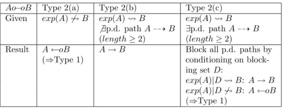
Ao−oB Type 2(a) Type 2(b) Type 2(c) Given exp(A) 6 B exp(A) B exp(A) B
6 ∃p.d. path A 99K B ∃p.d. path A 99K B (length ≥ 2) (length ≥ 2)
Result A←oB A→ B Block all p.d. paths by (⇒Type 1) conditioning on
block-ing set D:
exp(A)|D B: A → B exp(A)|D 6 B: A ←oB (⇒Type 1)
Table 2. An overview of how to complete edges of type o−o.
If at least one p.d. path Vi99K Vj exists, we need to block the influence of those paths on Vj while performing the experiment, so we try to find a blocking set D for all these paths. If exp(Vi)|D Vj, then the influence has to be immediate, because all paths of length ≥ 2 are blocked, so Vi → Vj. On the other hand if exp(Vi)|D 6 Vj, there is no immediate influence and the edge is Vi ↔ Vj (Type 1(c)).
Solving o
−o
An overview of the different rules for solving o−o is given in Table 2. For any edge Vio−oVj, we have no information at all, so we might need to perform experiments on both variables.
If exp(Vi) 6 Vj, then there is no influence of Vi on Vj so we know that there can be no directed edge between Viand Vj and thus the edge is of the following form: Vi←oVj, which then becomes a problem of Type 1.
If exp(Vi) Vj, then we know for sure that there is an influence of Vi on Vj, and like with Type 1(b) we make a difference whether there is a potentially directed path between Viand Vjof length ≥ 2, or not. If no such path exists, then the influence has to be immediate and the edge becomes Vi→ Vj.
If at least one p.d. path Vi99K Vj exists, we need to block the influence of those paths on Vjwhile performing the experiment, so we find a blocking set D like with Type 1(c). If exp(Vi)|D Vj, then the influence has to be immediate, because all paths of length ≥ 2 are blocked, so Vi → Vj. On the other hand if exp(Vi)|D 6 Vj, there is no immediate influence and the edge is of the following form: Vi←oVj, which again becomes a problem of Type 1.
V1 V2
V3 V4
V1 V2
V3 V4
(a) (b)
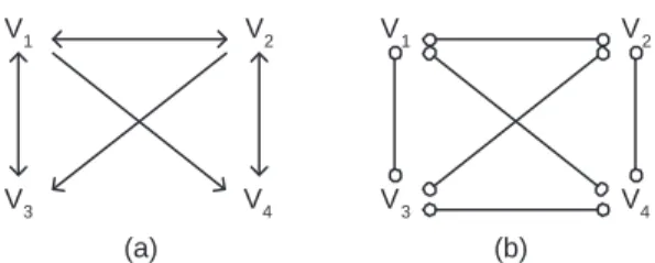
Figure 2. (a) A SMCM. (b) Result of FCI, with an i-false edge V3o−oV4.
Removing inducing path edges
An inducing path between two variables Vi and Vj might create an edge between these two variables during learning because the two are dependent conditional on any subset of observable variables. As mentioned before, this type of edges is not present in SMCMs as it does not represent an immediate causal influence or a latent variable in the underlying DAG. We will call such an edge an i-false edge.
For instance in Figure 1(a), the path V1, V2, L1, V6 is an inducing path, which causes the FCI algorithm to find an i-false edge between V1 and V6, see Figure 1(c). Another example is given in Figure 2 where the SMCM is given in (a) and the result of FCI in (b). The edge between V3 and V4 in (b) is a consequence of the inducing path via the observable variables V3, V1, V2, V4.
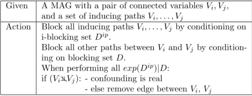
In order to be able to apply a causal inference algorithm we need to remove all i-false edges from the learned structure. We need to identify the substructures that can indicate this type of edges. This is easily done by looking at any two variables that are connected by an immediate connection, and when this edge is removed, they have at least one inducing path between them. To check whether the immediate connection needs to be present we have to block all inducing paths by performing one or more experiments on an inducing path blocking set (i-blocking set) Dip and block all other paths by conditioning on a blocking set D. If Vi and Vj are dependent, i.e. (Vi 2Vj) under these circumstances then the edge is correct and otherwise it can be removed.
In the example of Figure 1(c), we can block the inducing path by per-forming an experiment on V2, and hence can check that V1 and V6 do not covary with each other in these circumstances, so the edge can be removed.
Given A MAG with a pair of connected variables Vi, Vj, and a set of inducing paths Vi, . . . , Vj
Action Block all inducing paths Vi, . . . , Vj by conditioning on i-blocking set Dip.
Block all other paths between Vi and Vj by condition-ing on blockcondition-ing set D.
When performing all exp(Dip)|D: if (Vi 2Vj): - confounding is real
- else remove edge between Vi, Vj Table 3. Removing i-false edges.
3.4 Example
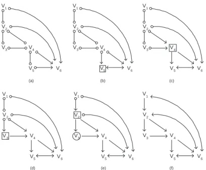
We will demonstrate a number of steps to discover the completely oriented SMCM (Figure 1(b)) based on the result of the FCI algorithm applied on observational data generated from the underlying DAG in Figure 1(a). The result of the FCI algorithm can be seen in Figure 3(a). We will first resolve problems of Type 1 and 2, and then remove i-false edges. The result of each step is explained in Table 4 and indicated in Figure 3.
Exper. Edge Experiment Edge Type before result after
exp(V5) V5o−oV4 exp(V5) 6 V4 V4o→ V5 Type 2(a) V5o→ V6 exp(V5) 6 V6 V5↔ V6 Type 1(a) exp(V4) V4o−oV2 exp(V4) 6 V2 V2o→ V4 Type 2(a) V4o−oV3 exp(V4) 6 V3 V3o→ V4 Type 2(a) V4o→ V5 exp(V4) V5 V4→ V5 Type 1(b) V4o→ V6 exp(V4) V6 V4→ V6 Type 1(b) exp(V3) V3o−oV2 exp(V3) 6 V2 V2o→ V3 Type 2(a) V3o→ V4 exp(V3) V4 V3→ V4 Type 1(b) exp(V2) V2o−oV1 exp(V2) 6 V1 V1o→ V2 Type 2(a) V2o→ V3 exp(V2) V3 V2→ V3 Type 1(b) exp(V2)|V3 V2o→ V4 exp(V2)|V3 V4 V2→ V4 Type 1(c) Table 4. Example steps in disambiguating edges by performing experiments.
After resolving all problems of Type 1 and 2 we end up with the SMCM structure shown in Figure 3(f), this representation is no longer consistent with the MAG representation since there are bi-directed edges between two variables on a directed path, i.e. V2, V6. There is a potentially i-false edge V1 ↔ V6 in the structure with inducing path V1, V2, V6, so we need to
V3 V1 V2 V5 V4 V6 V3 V1 V2 V5 V4 V6 V3 V1 V2 V5 V4 V6 (b) (c) (d) (e) V3 V1 V2 V5 V4 V6 V3 V1 V2 V5 V4 V6 (f) V3 V1 V2 V5 V4 V6 (a)
Figure 3. (a) The result of FCI on data of the underlying DAG of Figure 1(a). (b) Result of an experiment at V5. (c) Result after experiment at V4. (d) Result after experiment at V3. (e) Result after experiment at V2 while conditioning on V3. (f) Result of resolving all problems of Type 1 and 2.
perform an experiment on V2, blocking all other paths between V1 and V6 (this is also done by exp(V2) in this case). Given that the original structure is as in Figure 1(a), performing exp(V2) shows that V1and V6are independent, i.e. exp(V2) : (V1⊥⊥V6). Thus the bi-directed edge between V1 and V6is removed, giving us the SMCM of Figure 1(b).
4
Parametrisation of SMCMs
As mentioned before, in his work on causal inference, Tian provides an algorithm for performing causal inference given knowledge of the structure of an SMCM and the joint probability distribution (JPD) over the observable variables. However, a parametrisation to efficiently store the JPD over the observables is not provided.
We start this section by discussing the factorisation for SMCMs intro-duced in Tian and Pearl (2002a). From that result we derive an additional representation for SMCMs and a parametrisation of that representation that facilitates probabilistic and causal inference. We will also discuss how these
parameters can be learned from data. 4.1 Factorising with Latent Variables
Consider an underlying DAG with observable variables V = {V1, . . . , Vn} and latent variables L = {L1, . . . , Ln′}. Then the joint probability
distrib-ution can be written as the following mixture of products:
P(v) = X {lk|Lk∈L}
Y Vi∈V
P(vi|P a(vi), LP a(vi))Y Lj∈L
P(lj). (1.1)
Remember that in a SMCM the latent variables are implicitly represented by bi-directed edges, then consider the following definition.
DEFINITION 1.8. In a SMCM, the set of observable variables can be par-titioned into disjoint groups by assigning two variables to the same group iff they are connected by a bi-directed path. We call such a group a c-component(from ”confounded component”) (Tian and Pearl, 2002a).
E.g. in Figure 1(b) variables V2, V5, V6 belong to the same c-component. Then it can be readily seen that c-components and their associated latent variables form respective partitions of the observable and latent variables. Let Q[Si] denote the contribution of a c-component with observable vari-ables Si ⊂ V to the mixture of products in equation 1.1. Then we can rewrite the JPD as follows: P (v) = Q
i∈{1,...,k} Q[Si].
Finally, Tian and Pearl (2002a) proved that each Q[S] could be calculated as follows. Let Vo1 < . . . < Von be a topological order over V , and let
V(i)= Vo1 < . . . < Voi, i = 1, . . . , n and V
(0)= ∅. Q[S] = Y
Vi∈S
P(vi|(Ti∪ P a(Ti))\{Vi}) (1.2)
where Tiis the c-component of the SMCM G reduced to variables V(i), that contains Vi. The SMCM G reduced to a set of variables V′⊂ V is the graph obtained by removing all variables V \V′ from the graph and the edges that are connected to them.
In the rest of this section we will develop a method for deriving a DAG from a SMCM. We will show that the classical factorisationQP(vi|P a(vi)) associated with this DAG, is the same as the one that is associated with the SMCM as above.
4.2 Parametrised representation
Here we first introduce an additional representation for SMCMs, then we show how it can be parametrised and finally, we discuss how this new rep-resentation could be optimised.
Given a SMCM G and a topological order O, the PR-representation has these properties: 1. The nodes are V , the observable variables of the SMCM. 2. The directed edges that are present in the SMCM are also
present in the PR-representation.
3. The bi-directed edges in the SMCM are replaced by a number of directed edges in the following way:
Add an edge from node Vi to node Vj iff:
a) Vi∈ (Tj∪ P a(Tj)), where Tj is the c-component of G reduced to variables V(j)that contains Vj,
b) except if there was already an edge between nodes Vi and Vj. Table 5. Obtaining the parametrised representation from a SMCM.
V3 V1 V2 V5 V4 V6 V1,V2,V4,V5,V6 V2,V4 V2,V3,V4 (a) (b)
Figure 4. (a) The PR-representation applied to the SMCM of Figure 1(b). (b) Junction tree representation of the DAG in (a).
PR-representation
Consider Vo1 < . . . < Von to be a topological order O over the observable variables V , and let V(i)= Vo
1 < . . . < Voi, i = 1, . . . , n and V
(0)= ∅. Then Table 5 shows how the parametrised (PR-) representation can be obtained from the original SMCM structure.
What happens is that each variable becomes a child of the variables it would condition on in the calculation of the contribution of its c-component as in Equation (1.2).
In Figure 4(a), the PR-representation of the SMCM in Figure 1(a) can be seen. The topological order that was used here is V1< V2< V3< V4< V5< V6and the directed edges that have been added are V1→ V5, V2→ V5, V1→ V6, V2→ V6, and, V5→ V6.
The result is a DAG that is an I -map (Pearl, 1988), over the observable variables of the independence model represented by the SMCM. This means that all the independencies that can be derived from the new graph must also be present in the JPD over the observable variables. It can be readily seen that this is the case in the new representation as on one hand, no edges are removed from the SMCM. On the other hand, bi-directed edges A↔ B are replaced by directed edges A → B, this could lead to conditional independencies in the DAG that were not present in the original SMCM. Therefore, all parents of A are connected with B in the PR-representation.
Parametrisation
For this DAG we can use the same parametrisation as for classical BNs, i.e. learning P (vi|P a(vi)) for each variable, where P a(vi) denotes the parents in the new DAG. In this way the JPD over the observable variables factorises as in a classical BN, i.e. P (v) =QP(vi|P a(vi)). This follows immediately from the definition of a c-component and from Equation (1.2).
Optimising the Parametrisation
Remark that the number of edges added during the creation of the PR-representation depends on the topological order of the SMCM.
As this order is not unique, giving precedence to variables with a lesser amount of parents, will cause less edges to be added to the DAG. This is be-cause added edges go from parents of c-component members to c-component members that are topological descendants.
By choosing an optimal topological order, we can conserve more condi-tional independence relations of the SMCM and thus make the graph more sparse, leading to a more efficient parametrisation.
Learning parameters
As the PR-representation of SMCMs is a DAG as in the classical Bayesian network formalism, the parameters that have to be learned are P (vi|P a(vi)). Therefore, techniques such as ML and MAP estimation (Heckerman, 1995) can be applied to perform this task.
4.3 Probabilistic inference
Two of the most famous existing probabilistic inference algorithms for mod-els without latent variables are the λ − π algorithm (Pearl, 1988) for tree-structured BNs, and the junction tree algorithm (Lauritzen and Spiegelhal-ter, 1988) for arbitrary BNs.
These techniques cannot immediately be applied to SMCMs for two rea-sons. First of all until now no efficient parametrisation for this type of models was available, and secondly, it is not clear how to handle the bi-directed edges that are present in SMCMs.
We have solved this problem by first transforming the SMCM to its PR-representation which allows us to apply the junction tree (JT) inference algorithm. This is a consequence of the fact that, as previously mentioned, the PR-representation is an I -map over the observable variables. And as the JT algorithm only uses independencies in the DAG, applying it to an I -map of the problem gives correct results. See Figure 4(b) for the junction tree obtained from the parametrised representation in Figure 4(a).
Note that any other classical probabilistic inference technique that only uses conditional independencies between variables could also be applied to the PR-representation.
4.4 Causal inference
In Tian and Pearl (2002a), an algorithm for performing causal inference was developed, however as mentioned before they have not provided an efficient parametrisation.
In Spirtes et al. (2000); Zhang (2006), a procedure is discussed that can identify a limited amount of causal inference queries. More precisely only those whose result is equal for all the members of a Markov equivalence class represented by a CPAG.
In Richardson and Spirtes (2003), causal inference in AGs is shown on an example, but a detailed approach is not provided and the problem of what to do when some of the parents of a variable are latent is not solved.
By definition in the PR-representation, the parents of each variable are exactly those variables that have to be conditioned on in order to obtain the factor of that variable in the calculation of the c-component, see Table 5 and Tian and Pearl (2002a). Thus, the PR-representation provides all the necessary quantitative information, while the original structure of the SMCM provides the necessary structural information, for Tian’s algorithm to be applied.
5
Conclusions and Perspectives
In this article we have proposed a number of solutions to problems that arise when using SMCMs in practice.
More precisely we showed that there is a big gap between the models that can be learned from data alone and the models that are used in theory. We showed that it is important to retrieve the fully oriented structure of a SMCM, and discussed how to obtain this from a given CPAG by performing experiments.
For future work we would like to relax the assumptions made in this article. First of all we want to study the implications of allowing two types of edges between two variables, i.e. confounding as well as a immediate
causal relationship. Another direction for possible future work would be to study the effect of allowing multiple joint experiments in other cases than when removing inducing path edges.
Furthermore, we believe that applying the orientation and tail augmen-tation rules of Zhang and Spirtes (2005a) after each experiment, might help to reduce the number of experiments needed to fully orient the structure. In this way we could extend our previous results (Meganck et al., 2006) on minimising the total number of experiments in causal models without latent variables, to SMCMs. This allows to compare practical results with the theoretical bounds developed in Eberhardt et al. (2005).
SMCMs have not been parametrised in another way than by the entire joint probability distribution, we showed that using an alternative represen-tation, we can parametrise SMCMs in order to perform probabilistic as well as causal inference. Furthermore this new representation allows to learn the parameters using classical methods.
We have informally pointed out that the choice of a topological order when creating the PR-representation, influences the size and thus the effi-ciency of the PR-representation. We would like to investigate this property in a more formal manner. Finally, we have started implementing the tech-niques introduced in this article into the structure learning package (SLP)1 of the Bayesian networks toolbox (BNT)2 for MATLAB.
Acknowledgements
This work was partially funded by a IWT-scholarship. This work was par-tially supported by the IST Programme of the European Community, un-der the PASCAL network of Excellence, IST-2002-506778. This publication only reflects the authors’ views.
1http://banquiseasi.insa-rouen.fr/projects/bnt-slp/ 2http://bnt.sourceforge.net/
BIBLIOGRAPHY
Ali, A. and Richardson, T. (2002). Markov equivalence classes for maxi-mal ancestral graphs. In Proc. of the 18th Conference on Uncertainty in Artificial Intelligence (UAI), pages 1–9.
Chickering, D. (2002). Learning equivalence classes of Bayesian-network structures. Journal of Machine Learning Research, 2:445–498.
Eberhardt, F., Glymour, C., and Scheines, R. (2005). On the number of ex-periments sufficient and in the worst case necessary to identify all causal relations among n variables. In Proc. of the 21st Conference on Uncer-tainty in Artificial Intelligence (UAI), pages 178–183.
Friedman, N. (1997). Learning belief networks in the presence of missing values and hidden variables. In Proc. of the 14th International Conference on Machine Learning.
Heckerman, D. (1995). A tutorial on learning with bayesian networks. Tech-nical report, Microsoft Research.
Lauritzen, S. L. and Spiegelhalter, D. J. (1988). Local computations with probabilities on graphical structures and their application to expert sys-tems. Journal of the Royal Statistical Society, series B, 50:157–244. Meganck, S., Leray, P., and Manderick, B. (2006). Learning causal bayesian
networks from observations and experiments: A decision theoretic ap-proach. In Modeling Decisions in Artificial Intelligence, LNCS.
Neapolitan, R. (2003). Learning Bayesian Networks. Prentice Hall. Pearl, J. (1988). Probabilistic Reasoning in Intelligent Systems. Morgan
Kaufmann.
Pearl, J. (2000). Causality: Models, Reasoning and Inference. MIT Press. Richardson, T. and Spirtes, P. (2002). Ancestral graph markov models.
Richardson, T. and Spirtes, P. (2003). Causal inference via Ancestral graph models, chapter 3. Oxford Statistical Science Series: Highly Structured Stochastic Systems. Oxford University Press.
Spirtes, P., Glymour, C., and Scheines, R. (2000). Causation, Prediction and Search. MIT Press.
Tian, J. and Pearl, J. (2002a). On the identification of causal effects. Tech-nical Report (R-290-L), UCLA C.S. Lab.
Tian, J. and Pearl, J. (2002b). On the testable implications of causal models with hidden variables. In Proc. of the 18th Conference on Uncertainty in Artificial Intelligence (UAI).
Zhang, J. (2006). Causal Inference and Reasoning in Causally Insufficient Systems. PhD thesis, Carnegie Mellon University.
Zhang, J. and Spirtes, P. (2005a). A characterization of markov equivalence classes for ancestral graphical models. Technical Report 168, Dept. of Philosophy, Carnegie-Mellon University.
Zhang, J. and Spirtes, P. (2005b). A transformational characterization of markov equivalence for directed acyclic graphs with latent variables. In Proc. of the 21st Conference on Uncertainty in Artificial Intelligence (UAI), pages 667–674.
Sam Maes- [email protected]
INSA Rouen - LITIS, BP 08 Av. de l’Universit´e, 76801 St-Etienne-du-Rouvray, France.
Stijn Meganck- [email protected]
Vrije Universiteit Brussel - CoMo, Pleinlaan 2, 1050 Brussel, Belgium. Philippe Leray- [email protected]
INSA Rouen - LITIS, BP 08 Av. de l’Universit´e, 76801 St-Etienne-du-Rouvray, France.