HAL Id: hal-01590892
https://hal.archives-ouvertes.fr/hal-01590892
Submitted on 20 Sep 2017
HAL is a multi-disciplinary open access
archive for the deposit and dissemination of
sci-entific research documents, whether they are
pub-lished or not. The documents may come from
teaching and research institutions in France or
abroad, or from public or private research centers.
L’archive ouverte pluridisciplinaire HAL, est
destinée au dépôt et à la diffusion de documents
scientifiques de niveau recherche, publiés ou non,
émanant des établissements d’enseignement et de
recherche français ou étrangers, des laboratoires
publics ou privés.
Consistency in Parametric Interval Probabilistic Timed
Automata
Etienne André, Benoit Delahaye
To cite this version:
Etienne André, Benoit Delahaye. Consistency in Parametric Interval Probabilistic Timed Automata.
23rd International Symposium on Temporal Representation and Reasoning, Oct 2016, Copenhagen,
Denmark. �hal-01590892�
Consistency in Parametric Interval Probabilistic Timed Automata
´
Etienne Andr´e
1Universit´e Paris 13, Sorbonne Paris Cit´e, LIPN CNRS, UMR 7030, F-93430, Villetaneuse, France 2Ecole Centrale de Nantes, IRCCyN, CNRS, UMR 6597, France´
Benoˆıt Delahaye Universit´e de Nantes
LINA UMR CNRS 6241, Nantes, France
Abstract—We propose a new abstract formalism for proba-bilistic timed systems, Parametric Interval Probaproba-bilistic Timed Automata, based on an extension of Parametric Timed Au-tomata and Interval Markov Chains. In this context, we con-sider the consistency problem that amounts to deciding whether a given specification admits at least one implementation. In the context of Interval Probabilistic Timed Automata (with no timing parameters), we show that this problem is decidable and propose a constructive algorithm for its resolution. We show that the existence of parameter valuations ensuring consistency is undecidable in the general context, but still propose a semi-algorithm that resolves it whenever it terminates.
Keywords-parametric verification; timed probabilistic sys-tems; parametric probabilistic timed automata;
I. INTRODUCTION
Motivation: Nowadays, automata-based modeling and verification methods are mainly used in two different ways: for designing digital systems based on (mostly informal) specifications expressed by the end-users of these systems or from the knowledge designers have of their environment; and in order to abstract existing (not necessarily software) systems that are too complex to comprehend in their entirety. In both cases the complexity of the systems being designed calls for increasingly expressive abstraction artifacts such as time and probabilities. Timed automata [1] are a widely recognized modeling formalism for reasoning about real-time systems. This modeling formalism, based on finite control automata equipped with clocks, which are real-valued variables which increase uniformly at the same rate, has been extended to the probabilistic framework in [2], [3]. In this context, discrete actions are replaced with probabilis-tic discrete distributions over discrete actions, allowing to model uncertainties in the system’s behavior. This formalism has been applied to a number of case studies [4].
Unfortunately, building a system model based either on imprecise specifications or on imprecise observations often requires to fix arbitrarily a number of constants in the model, which are then calibrated by a fastidious comparison of the model behavior and the expected behavior. This is the case for instance for timing constants or transition probability values. In order to incorporate these uncertainties in the This work is partially supported by the ANR national research program PACS (ANR-14-CE28-0002).
model and to develop automatic calibration, more abstract formalisms have been introduced separately in the timed setting and in the probabilistic setting.
In the timed setting, parametric timed automata [5] allow using parameter variables in the guards of timed transitions in order to account for the uncertainty on their values. Para-metric probabilistic timed automata were proposed in [6] to answer the following question: given a parameter valuation, what are other valuations preserving the same minimum and maximum probabilities for reachability properties as the reference valuation? Parametric probabilistic timed automata were then given a symbolic semantics in [7]; a method has been proposed in that same work to synthesize optimal pa-rameter valuations to maximize or minimize the probability of reaching a discrete location.
In the pure probabilistic setting, Interval Markov Chains (IMCs for short) have been introduced [8] to take into account imprecision in the transition probabilities. IMCs extend Markov Chains by allowing to specify intervals of possible probabilities on transitions instead of exact values. Methods have then been developed to decide whether there exists Markov Chains with concrete probability values that match the intervals specified in a given IMC [9].
Contribution: In this paper, we propose to combine both abstraction approaches into a single specification theory: Parametric Interval Probabilistic Timed Automata (PIℙTAs for short). In this setting, parameters can be used in order to abstract timed constants on transition guards while intervals can be used to abstract imprecise transition probabilities. As for IMCs, it is important to be able to decide whether the probability intervals that are specified in a model allow defining coherent probability distributions (i. e., can be matched in a real-life implementation). This is called the consistency problem. In the context of Interval Probabilistic Timed Automata with no timing parameters (IℙTAs for short), we propose an algorithm that resolves this problem. In our setting, since the behavior of the system is conditioned by the calibration of parameter values, it is therefore necessary to decide whether there exist parameter values that ensure consistency of the resulting model (and synthesize these values when this is possible). We show that the existence of such parameter valuations is undecidable in the general context of PIℙTAs. Still, we propose a
semi-algorithm that synthesizes, whenever it terminates, the set of parameter values that ensure consistency of the resulting IℙTA.
Outline: We start II with preliminary definitions and then introduce the concepts of IℙTAs and PIℙTAs. In III, we study the consistency problem for IℙTAs and propose a constructive algorithm based on the zone-graph construction that decides whether an IℙTA is consistent and produces an implementation if one exists. In IV, we move to the general problem of consistency of PIℙTAs. We first show that this problem is undecidable in general and then propose a semi-algorithm that synthesizes, whenever it terminates, the set of parameter values ensuring consistency of the resulting IℙTA. Finally, V concludes the paper.
II. PRELIMINARIES A. Clocks, Parameters and Constraints
Let ℕ, ℤ, ℚ+ and ℝ+ denote the sets of non-negative integers, integers, negative rational numbers and non-negative real numbers respectively. Given an arbitrary set 𝑆, we write Dist(𝑆) for the set of probabilistic distributions over𝑆.
Throughout this paper, let 𝑋 = {𝑥1, . . . , 𝑥𝐻} be a set of clocks, i. e., real-valued variables that evolve at the same rate, and Γ = {𝛾1, . . . , 𝛾𝑀} be a set of parameters, i. e., unknown constants.
A clock valuation is a function𝑤 : 𝑋 → ℝ+. We identify a clock valuation𝑤 with the point (𝑤(𝑥1), . . . , 𝑤(𝑥𝐻)). We write ⃗0 for the valuation that assigns 0 to each clock. Given 𝑑 ∈ ℝ+,𝑤 +𝑑 denotes the valuation such that (𝑤 +𝑑)(𝑥) = 𝑤(𝑥) + 𝑑, for all 𝑥 ∈ 𝑋. Given 𝜌 ⊆ 𝑋, we define [𝑤]𝜌 as
the clock valuation obtained by resetting the clocks in𝜌 and keeping other clocks unchanged.
A parameter valuation 𝑣 is a function 𝑣 : Γ → ℚ+. We identify a parameter valuation 𝑣 with the point (𝑣(𝛾1), . . . , 𝑣(𝛾𝑀)).
In the following, we assume ≺ ∈ {<, ≤} and ∼ ∈ {< , ≤, ≥, >}. lt denotes a linear term over 𝑋 ∪ Γ of the form ∑
1≤𝑖≤𝐻𝛼𝑖𝑥𝑖+∑1≤𝑗≤𝑀𝛽𝑗𝛾𝑗+ 𝑑, with 𝑥𝑖∈ 𝑋, 𝛾𝑗 ∈ Γ,
and𝛼𝑖, 𝛽𝑗, 𝑑 ∈ ℤ. plt denotes a parametric linear term over Γ, that is a linear term without clocks (𝛼𝑖 = 0 for all 𝑖).
A constraint 𝐶 over 𝑋 ∪ Γ is a conjunction of inequalities of the form lt ∼ 0 (i. e., a convex polyhedron). Given a parameter valuation𝑣, 𝑣(𝐶) denotes the constraint over 𝑋 obtained by replacing each parameter 𝛾 in 𝐶 with 𝑣(𝛾). Likewise, given a clock valuation 𝑤, 𝑤(𝑣(𝐶)) denotes the expression obtained by replacing each clock 𝑥 in 𝑣(𝐶) with 𝑤(𝑥). We say that 𝑣 satisfies 𝐶, denoted by 𝑣 ∣= 𝐶, if the set of clock valuations satisfying 𝑣(𝐶) is nonempty. Given a parameter valuation 𝑣 and a clock valuation 𝑤, we denote by 𝑤∣𝑣 the valuation over 𝑋 ∪ Γ such that for all clocks 𝑥, 𝑤∣𝑣(𝑥) = 𝑤(𝑥) and for all parameters 𝛾, 𝑤∣𝑣(𝛾) = 𝑣(𝛾). We use the notation 𝑤∣𝑣 ∣= 𝐶 to indicate that𝑤(𝑣(𝐶)) evaluates to true. We say that 𝐶 is satisfiable
if ∃𝑤, 𝑣 s. t.𝑤∣𝑣 ∣= 𝐶. We define the time elapsing of 𝐶, denoted by 𝐶↗, as the constraint over 𝑋 and Γ obtained from 𝐶 by delaying all clocks by an arbitrary amount of time. Given𝜌 ⊆ 𝑋, we define the reset of 𝐶, written [𝐶]𝜌, as the constraint obtained from𝐶 by resetting the clocks in 𝜌, and keeping the other clocks unchanged. We denote by𝐶↓Γ the projection of𝐶 onto Γ, i. e., obtained by eliminating the clock variables (e. g., using the Fourier-Motzkin algorithm). A guard𝑔 is a constraint over 𝑋 ∪ Γ defined by inequal-ities of the form 𝑥 ∼ 𝑧, where 𝑧 is either a parameter or a constant inℤ.
A zone is a polyhedron over a set of clocks in which all constraints on variables are of the form 𝑥 ∼ 𝑘 (rectangular constraints) or 𝑥𝑖− 𝑥𝑗 ∼ 𝑘 (diagonal constraints), where 𝑥𝑖 ∈ 𝑋, 𝑥𝑗 ∈ 𝑋 and 𝑘 is an integer. Operations on zones
are well-documented (see e. g., [10]).
A parametric zone is a convex polyhedron over 𝑋 ∪ Γ in which all constraints on variables are of the form 𝑥 ∼ plt (parametric rectangular constraints) or 𝑥𝑖 − 𝑥𝑗 ∼ plt
(parametric diagonal constraints), where 𝑥𝑖 ∈ 𝑋, 𝑥𝑗 ∈ 𝑋 andplt is a parametric linear term over Γ. We denote the set of all parametric zones by𝒵.
B. Timed Probabilistic Systems
We review the definition of timed probabilistic systems, as defined in [3]. A timed probabilistic system (TPS) is a tuple𝒯 = (𝑆, 𝑠0, Σ, ⇒) where 𝑆 is a set of states, 𝑠0∈ 𝑆 is the initial state, Σ is a finite set of actions, and ⇒ ⊆ 𝑆 × ℝ+× Σ × Dist(𝑆) is a probabilistic transition relation. C. Probabilistic Timed Automata
Probabilistic timed automata [2], [3] are an extension of classical timed automata [1] with discrete probability distributions
1) Syntax:
Definition 1. A Probabilistic Timed Automaton (ℙTA) 𝒫 is
a tuple (Σ, 𝐿, 𝑙0, 𝑋, 𝑝𝑟𝑜𝑏), where: i) Σ is a finite set of actions, ii) 𝐿 is a finite set of locations, iii) 𝑙0 ∈ 𝐿 is the initial location, iv) 𝑋 is a finite set of clocks, v) 𝑝𝑟𝑜𝑏 is a probabilistic edge relation consisting of elements of the form (𝑙, 𝑔, 𝑎, 𝜇), where 𝑙 ∈ 𝐿, 𝑔 is a constraint on the clocks 𝑋, 𝑎 ∈ Σ, and 𝜇 ∈ Dist(2𝑋× 𝐿).
Note that we use no invariant; this is an important condition for the correctness of our techniques. However, invariants can be eliminated (moved to the guards prior to the transition), following classical techniques defined for (probabilistic) timed automata.
We use the following conventions for the graphical rep-resentation of probabilistic timed automata: locations are represented by nodes, within which name of the location is written; probabilistic edges are represented by arcs from locations, labeled by the associated guard and action, and which split into multiple arcs, each of which leads to a
location and which is labeled by a set of clocks to be reset to 0 and a probability (probabilistic edges which correspond to probability 1 are illustrated by a single arc from location to location).
Example 1. 1a presents an example of a ℙTA with two
clocks 𝑥 and 𝑦. For example, 𝑙0 can be exited whenever 𝑦 < 2; then, with probability 0.4 the target location becomes 𝑙2, resetting 𝑥; or with probability 0.6 the target location is 𝑙1, resetting 𝑦. The transition from 𝑙2 can be explained similarly.
2) Semantics of ℙTAss: A ℙTA can be interpreted as an infinite TPS. Due to the continuous nature of clocks, the underlying TPS has uncountably many states, and is uncountably branching.
Definition 2 (Concrete semantics of a ℙTA). Given a ℙTA
𝒫 = (Σ, 𝐿, 𝑙0, 𝑋, 𝑝𝑟𝑜𝑏), the concrete semantics of 𝒫 is given by the timed probabilistic system𝒯𝒫 = (𝑆, 𝑠0, Σ, ⇒), with
∙ 𝑆 = {(𝑙, 𝑤) ∈ 𝐿 × ℝ𝐻+} , 𝑠0= (𝑙0,⃗0)
∙ ((𝑙, 𝑤), 𝑑, 𝑎, 𝜇) ∈ ⇒ if both of the following conditions
hold:
– time elapse:∀𝑑′ ∈ [0, 𝑑], (𝑙, 𝑤 + 𝑑′) ∈ 𝑆, and – edge traversal: there exists a probabilistic edge𝑒 =
(𝑙, 𝑔, 𝑎, 𝜂) ∈ 𝑝𝑟𝑜𝑏 such that 𝑤 + 𝑑 ∣= 𝑔 and, for each 𝑙′∈ 𝐿 and 𝜌 ⊆ 𝑋, 𝜂(𝜌, 𝑙′) = 𝜇(𝑙′, [𝑤 + 𝑑]𝜌).
Note that, due to the fact that we have no invariants, the first condition (time elapse) is always trivially true. D. Parametric Interval Probabilistic Timed Automata
In this section, we introduce basic definitions for (para-metric) interval probabilistic timed automata, that extend (parametric) probabilistic timed automata by providing in-tervals for transition probabilities instead of exact proba-bility values. In the spirit of (parametric) Interval Markov Chains [11], [12], (parametric) interval probabilistic timed automata are used for specifying potentially infinite families (sets) of probabilistic timed automata – those whose exact probability values match the specified intervals – with a finite structure of similar form.
1) Syntax: Given an arbitrary set 𝑆, we call an interval distribution over𝑆 a function Υ that assigns to each element of 𝑆 an interval of probabilities [𝑎, 𝑏] ⊆ [0, 1]. Intuitively, an interval distribution Υ over 𝑆 represents the set of all distributions𝜇 ∈ Dist(𝑆) that assign to each element 𝑠 ∈ 𝑆 a probability𝜇(𝑠) such that 𝜇(𝑠) ∈ Υ(𝑠). Formally, we define the implementation of an interval distribution as follows. Definition 3 (Implementation of an interval distribution).
Let𝑆 be an arbitrary set. Given an interval distribution Υ ∈ Int[0,1](𝑆), 𝜇 ∈ Dist(𝑆) is an implementation of Υ, written 𝜇 ∈ Υ iff, for all 𝑠 ∈ 𝑆, we have 𝜇(𝑠) ∈ Υ(𝑠).
In the rest of the paper, we writeInt[0,1](𝑆) for the set of interval distributions over𝑆. We now move to the definition
of (parametric) interval probabilistic timed automata. Definition 4. A Parametric Interval Probabilistic Timed
Au-tomaton (PIℙTA) 𝒫ℐ𝒫 is a tuple (Σ, 𝐿, 𝑙0, 𝑋, Γ, 𝕀), where: i)Σ is a finite set of actions, ii) 𝐿 is a finite set of locations, iii) 𝑙0 ∈ 𝐿 is the initial location, iv) 𝑋 is a finite set of clocks, v)Γ is a finite set of parameters, vi) 𝕀 is an interval-valued probabilistic edge relation consisting of elements of the form(𝑙, 𝑔, 𝑎, Υ), where 𝑙 ∈ 𝐿, 𝑔 is a guard, 𝑎 ∈ Σ, and Υ ∈ Int[0,1](2𝑋× 𝐿) is an interval distribution.
Given a PIℙTA 𝒫ℐ𝒫 = (Σ, 𝐿, 𝑙0, 𝑋, Γ, 𝕀) and a parameter valuation𝑣, the valuation of 𝒫ℐ𝒫 with 𝑣, written 𝑣(𝒫ℐ𝒫), is an Interval Probabilistic Timed Automaton (IℙTA) ℐ𝒫 = (Σ, 𝐿, 𝑙0, 𝑋, 𝕀′), where 𝕀′ is obtained by replacing within𝕀 any occurrence of a parameter 𝛾 with 𝑣(𝛾) and removing all transitions(𝑙, 𝑔, 𝑎, Υ) such that 𝑣(𝑔) ≡ ⊥ (technically, this latter part is not strictly speaking necessary, but it syntactically reduces a bit the model).
Remark that IℙTAs are very similar to ℙTAs: the only dif-ference is that probabilistic edges are labeled with intervals instead of exact probability values.
Once a parameter valuation is fixed, the resulting IℙTA represents a potentially infinite set ofℙTAs. In order to relate a given IℙTA with the ℙTA it represents, we use the notion of implementation defined hereafter. This notion is similar to the one defined in the context of (parametric) Interval Markov Chains [11], [12]. Remark that aℙTA implementing an IℙTA needs to conserve the exact same clocks, guards and resets.
Definition 5 (Implementation of an IℙTA). Let 𝒫 = (Σ, 𝐿, 𝑙0, 𝑋, 𝑝𝑟𝑜𝑏) be a ℙTA and ℐ𝒫 = (Σ, 𝐿′, 𝑙′
0, 𝑋, 𝕀) be an IℙTA.
We say that 𝒫 is an implementation of ℐ𝒫, written 𝒫 ∣= ℐ𝒫, iff there exists a relation ℛ ⊆ 𝐿′ × 𝐿, called
an implementation relation s. t. (𝑙′0, 𝑙0) ∈ ℛ and, whenever (𝑙′, 𝑙) ∈ ℛ, we have
∙ ∀(𝑙′, 𝑔′, 𝑎, 𝜇) ∈ 𝑝𝑟𝑜𝑏, ∃(𝑙, 𝑔′, 𝑎, Υ) ∈ 𝕀 s. t. 𝜇 ⪯ℛ Υ,
and
∙ ∀(𝑙, 𝑔, 𝑎, Υ) ∈ 𝕀, ∃(𝑙′, 𝑔, 𝑎, 𝜇) ∈ 𝑝𝑟𝑜𝑏 s. t. 𝜇 ⪯ℛΥ.
where𝜇 ⪯ℛ Υ iff ∃𝛿 ∈ Dist(𝐿′× 𝐿) s. t.
∙ ∀(𝜌′, 𝑙′) ∈ 2𝑋×𝐿′, 𝜇(𝜌′, 𝑙′) > 0 ⇒∑𝑙∈𝐿(𝛿(𝑙′, 𝑙)) = 1, ∙ ∀(𝜌, 𝑙) ∈ 2𝑋 × 𝐿,∑𝑙′∈𝐿′(𝜇(𝜌, 𝑙′) ⋅ 𝛿(𝑙′, 𝑙)) ∈ Υ(𝜌, 𝑙),
and
∙ 𝛿(𝑙′, 𝑙) > 0 ⇒ (𝑙′, 𝑙) ∈ ℛ.
Given an IℙTA, deciding whether the family it represents is nonempty is a nontrivial problem. Indeed, the inter-val distributions used throughout its structure could repre-sent contradictory constraints on the transition probabilities, therefore preventing anyℙTA from implementing it. Definition 6 (Consistency of an IℙTA). An IℙTA is
𝑙0 𝑙1 𝑙2 𝑙5 𝑦 < 2 𝑎 0.6 𝑦 := 0 0.4 𝑥 := 0 𝑥 = 1 ∧ 𝑦 ≤ 2 𝑐 0.1 𝑥 := 0 0.9 (a) AℙTA 𝑙0 𝑙1 𝑙2 𝑙5 𝑙3 𝑙4 𝑦 < 2 𝑎 [0, 1] 𝑦 := 0 [0, 0.5] 𝑥 := 0 2 ≤ 𝑥 ≤ 𝛾 𝑏 [0, 0.2] 𝑦 := 0 [0, 0.3] 𝑥, 𝑦 := 0 𝑥 = 1 ∧ 𝑦 ≤ 2 𝑐 0.1 𝑥 := 0 0.9 𝑥 = 5 𝑑 𝑥, 𝑦 := 0 2 ≤ 𝑥 ≤ 𝛾 𝑒 𝑥 := 0 (b) A PIℙTA Figure 1: Examples
Example 2. Consider the PIℙTA 𝒫ℐ𝒫 given in 1b, and
containing a single parameter𝛾. When the interval associ-ated with a distribution is reduced to a point (e. g.,[0.9, 0.9] from𝑙2to𝑙5), we simply represent it using its punctual value (i. e., 0.9). When a distribution is made of a single target location with probability 1, we simply omit the distribution (e. g., between𝑙3 to𝑙4).
Let 𝑣1 be the parameter valuation such that 𝑣1(𝛾) = 1. In the IℙTA 𝑣1(𝒫ℐ𝒫), the transition outgoing from 𝑙1 can never be taken, as its guard becomes 2 ≤ 𝑥 ≤ 1, which is unsatisfiable. Then, it is clear that the ℙTA 𝒫 given in 1a is an implementation of 𝑣1(𝒫ℐ𝒫). As a consequence, 𝑣1(𝒫ℐ𝒫) is a consistent IℙTA.
An important problem is therefore to decide whether a given IℙTA is consistent, which we address in the next section.
III. THECONSISTENCYPROBLEM FORIℙTAS In this section, we address the problem of deciding whether a given IℙTA is consistent. Unlike in the context of IMCs, where it is proven that a given IMC is consistent iff it admits an implementation with the same structure, a given IℙTA can be consistent but still not admit any implementation that respects its structure. Since transitions can be removed because their guard becomes unsatisfiable due to parameter valuations, the structure of implementations can differ from the one of the specification. Algorithms such as those proposed for deciding consistency of (p)IMCs in [12] therefore cannot be directly adapted to the IℙTAs setting as they are dependent on this property.
Fortunately, the operational semantics of IℙTAs can be expressed in terms of Interval Markov Decision Processes (IMDPs), which are similar to IMCs and satisfy the same structural properties regarding consistency. We therefore propose an algorithm for deciding consistency of IℙTAs based on the consistency of their symbolic IMDP
seman-tics. We start with preliminary definitions on IMDPs, then formally define the symbolic semantics of IℙTAs and finally propose an algorithm for deciding whether a given IℙTA is consistent.
A. Preliminary Definitions
An IMDP is a tuple (𝑆, 𝑠0, Σ, 𝑇 ) where 𝑆 is a set of states,𝑠0∈ 𝑆 is the initial state, Σ is a finite set of actions and 𝑇 ⊆ 𝑆 × Σ × Int[0,1](𝑆) is a probabilistic (interval) transition relation.
Example 3. 2b depicts an example of an IMDP. Just as
for IℙTAs, when the interval associated with a distribution is reduced to a point (e. g., [0.9, 0.9] from s2 to s5), we simply represent it using its punctual value (i. e.,0.9). When a distribution is made of a single target location with probability 1, we simply omit the distribution (e. g., between
s3 tos4).
An MDP is an IMDP such that for each(𝑠, 𝑎, [𝑚, 𝑛]) ∈ 𝑇 , we have𝑚 = 𝑛, and for each 𝑠 ∈ 𝑆,∑(𝑠,𝑎,𝑠′,[𝑚,𝑛])∈𝑇𝑚 =
1.
Example 4. 2a depicts an example of an MDP.
Definition 7 (implementation of an IMDP). Let ℐℳ = (𝑆, 𝑠0, Σ, 𝑇 ) be an IMDP. Let ℳ = (𝑆′, 𝑠′
0, Σ, 𝑇′) be an MDP. We say thatℳ is an implementation of ℐℳ, written ℳ ∣= ℐℳ, if ∃ℛ ⊆ 𝑆′×𝑆 s. t. (𝑠′
0, 𝑠0) ∈ ℛ and (𝑠′, 𝑠) ∈ ℛ if
∙ ∀(𝑠′, 𝑎, 𝜇) ∈ 𝑇′, ∃(𝑠, 𝑎, 𝐼) ∈ 𝑇 s. t. 𝜇 ⪯ℛ𝐼, and ∙ ∀(𝑠, 𝑎, 𝐼) ∈ 𝑇, ∃(𝑠′, 𝑎, 𝜇) ∈ 𝑇′ s. t.𝜇 ⪯ℛ𝐼.
As for IℙTAs, we say that an IMDP is consistent iff it admits at least one implementation.
Example 5. The IMDP given in 2b admits no
implemen-tation: indeed, on the (single) transition labeled with 𝑒2, no valuation of the two intervals[0, 0.3] and [0, 0.2] is such that the sum of both valuations is equal to 1. In addition, the
s0 s1 s2 s5 s6 s7 s8 𝑒1 0.6 0.4 𝑒3 0.1 0.9 𝑒3 0.1 0.9 (a) An example of an MDP s0 s1 s2 s5 s6 s7 s8 s3 s4 𝑒1 [0, 1] [0, 0.5] 𝑒2 [0, 0.2] [0, 0.3] 𝑒3 0.1 0.9 𝑒3 𝑒4 𝑒5 0.1 0.9 (b) An example of an IMDP Figure 2: Examples
transition from 𝑠0 to𝑠1 cannot be eliminated by assigning a 0-probability to that target state; although this would be compatible with the interval (0 ∈ [0, 1]), the second interval (to𝑠2) does not accept a 1-probability since its probability must be within[0, 0.5].
As said above IMDPs satisfy the same structural property as IMCs concerning implementations: they are consistent iff they admit at least one implementation that respects their structure. This result is formalized in the following lemma. Lemma 1 (structure of an implementation). An IMDPℐℳ
is consistent iff there exists an MDP ℳ with the same structure s. t.ℳ ∣= ℐℳ.
Proof:
Letℐℳ = (𝑆, 𝑠0, Σ, 𝑇 ) be an IMDP.
One direction of this result is trivial: if there exists an MDP ℳ with the same structure as ℐℳ s. t. ℳ ∣= ℐℳ, thenℐℳ is clearly consistent.
The reverse implication is more involved. Assume that ℐℳ is consistent, i. e., there exists an MDP ℳ = (𝑆′, 𝑠′
0, Σ, 𝑇′), with no assumption on its structure, such that ℳ ∣= ℐℳ. We then have to build an MDP ℳ∗ = (𝑆, 𝑠0, Σ, 𝑇∗) such that ℳ∗andℳ have the same structure.
Observe that 𝑆 and 𝑠0 must be identical to that of ℐℳ because they have the same structure.
Letℛ be the relation witnessing that ℳ ∣= ℐℳ and let 𝑓 : 𝑆 → 𝑆′ be a partial function that associates to each
state in ℐℳ one of the states from ℳ that contributes to its implementation, if any. Formally, for all 𝑠 ∈ 𝑆, if 𝑓(𝑠) is defined then(𝑓(𝑠), 𝑠) ∈ ℛ.
The transition relation 𝑇∗ of ℳ∗ is constructed as follows: For each state 𝑠 that is implemented, i. e., such that 𝑓(𝑠) is defined, and probabilistic interval transition (𝑠, 𝑎, 𝐼) ∈ 𝑇 in ℐℳ, we build a corresponding transition (𝑠, 𝑎, 𝜇𝐼) in ℳ∗ from the transitions inℳ that implement
(𝑠, 𝑎, 𝐼). States that are not implemented do not serve for consistency and are therefore not considered.
Formally, let (𝑠1, 𝑎, 𝐼) ∈ 𝑇 be a probabilistic interval
transition in ℐℳ. From 7, we know that there exists (𝑓(𝑠1), 𝑎, 𝜇) ∈ 𝑇′ s. t. 𝜇 ⪯ℛ 𝐼. Let 𝛿 be the function
given by𝜇 ⪯ℛ𝐼. The distribution 𝜇𝐼 is then constructed as follows: for all𝑠2∈ 𝑆, let 𝜇𝐼(𝑠2) =∑𝑠′∈𝑆′𝜇(𝑠′)⋅𝛿(𝑠′, 𝑠2).
By definition of 𝛿, observe that 𝜇𝐼(𝑠2) ∈ 𝐼(𝑠2) for all 𝑠2∈ 𝑆 and that, whenever 𝜇𝐼(𝑠2) > 0, 𝑓(𝑠2) is defined.
Clearly,ℳ∗is therefore an implementation ofℐℳ, with witnessing relation ℛ∗ the identity relation on the set of states𝑠 ∈ 𝑆 such that 𝑓(𝑠) is defined.
B. A Symbolic Semantics for IℙTAs
We equip IℙTAs with a symbolic semantics, defined below. Basically, it is inline with the symbolic semantics defined for timed automata, with the addition of probabilistic intervals on the edges; as a consequence, the semantics becomes not an LTS, but an IMDP.
Definition 8 (Symbolic semantics of an IℙTA). Given an
IℙTA ℐ𝒫 = (Σ, 𝐿, 𝑙0, 𝑋, 𝕀), the symbolic semantics of ℐ𝒫 is given by the IMDP(S, s0, Σ, 𝑇 ), with
∙ S = {(𝑙, 𝐶) ∈ 𝐿 × 𝒵}, s0= (𝑙0, (⋀1≤𝑖≤𝐻𝑥𝑖= 0)↗), ∙ (s, 𝑒 , Υ′) ∈ 𝑇 if 𝑒 = (𝑙, 𝑔, 𝑎, Υ) ∈ 𝕀 and for all 𝑙′∈ 𝐿,
for all𝜌 ⊆ 𝑋 such that Υ(𝑙′, 𝜌) > 0, 𝐶′=([𝐶∧𝑔]𝜌)↗, and Υ′((𝑙′, 𝐶′)) = Υ(𝑙′, 𝜌).
Observe that, whenever an IℙTA has no probabilistic choice, then the IMDP becomes a labeled transition system, and the symbolic semantics matches that of timed automata given in the form of a zone graph [10]. It is well-know that the zone graph of a timed automaton can have an infinite number of states; however, applying the classical 𝑘-extrapolation (that basically splits zones between a part where the clock constraints are smaller or equal to 𝑘 and a part where constraints are larger than 𝑘, where 𝑘 is the largest integer-constant in the timed automaton) yields termination (see, e. g., [13]). In the following, we apply the classical𝑘-extrapolation to the symbolic constraints of the semantics of an IℙTA ℐ𝒫, and therefore the number of states in the IMDP described in 8 is finite. We refer to the symbolic semantics ofℐ𝒫 as the probabilistic zone graph of ℐ𝒫.
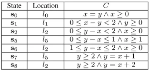
State Location 𝐶 s0 𝑙0 𝑥 = 𝑦 ∧ 𝑥 ≥ 0 s1 𝑙1 0 ≤ 𝑥 − 𝑦 < 2 ∧ 𝑦 ≥ 0 s2 𝑙2 0 ≤ 𝑦 − 𝑥 < 2 ∧ 𝑥 ≥ 0 s5 𝑙5 0 ≤ 𝑦 − 𝑥 ≤ 1 ∧ 𝑥 ≥ 1 s6 𝑙2 1 ≤ 𝑦 − 𝑥 ≤ 2 ∧ 𝑥 ≥ 0 s7 𝑙5 𝑦 ≥ 2 ∧ 𝑦 = 𝑥 + 1 s8 𝑙2 𝑦 ≥ 2 ∧ 𝑦 = 𝑥 + 2
Table I: Description of the states in 2a
Remark that the probabilistic zone graph is defined for IℙTAs in the form of an IMDP; a ℙTA can be understood as an IℙTA, and its associated zone graph becomes an MDP. Example 6. The probabilistic zone graph of theℙTA in 1a
is the MDP given in 2a. The symbolic states s𝑖 = (𝑙𝑖, 𝐶𝑖) are expanded in I.
C. Reconstructing a ℙTA from a Probabilistic Zone Graph It is well-known that, given a timed automata𝒜 and its zone graph, a second timed automaton 𝒜′ can be recon-structed from the zone graph, with the same structure as the zone graph, and such that the zone graph of𝒜′ is the same as that of𝒜. We extend this technique here to ℙTAs.
Let 𝒫 be a ℙTA and let ℳ be its probabilistic zone graph. Let us build a second ℙTA 𝒫′. Each state of ℳ is translated into a location of𝒫′. Then, for each transition (s, 𝑒 , Υ′) ∈ 𝑇 in ℳ, where 𝑒 = (𝑙, 𝑔, 𝑎, Υ), we create a
transition (𝑙, 𝑔, 𝑎, Υ), where Υ is defined exactly as in 𝒫, except that the target location matches the target state inℳ (a single location in 𝒫 can yield different states in ℳ). Following results for timed automata, the probabilistic zone graph of𝒫′ isℳ.
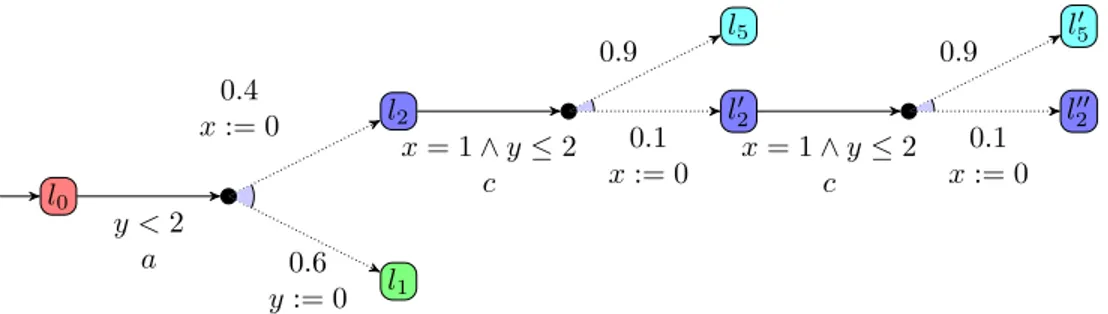
Example 7. The ℙTA reconstructed from the probabilistic
zone graph in 2a is given in 3. Its probabilistic zone graph is again that of 2a.
D. An Algorithm for the Consistency of IℙTAs
We start with the following observation: by construction, the purpose of the symbolic semantics of IℙTAs is to represent, at a lower level of abstraction, the same set of objects. Intuitively, the symbolic IMDP semantics of a given IℙTA should therefore be consistent iff the original IℙTA is itself consistent. This result is formally proven in the following theorem.
Theorem 1. An IℙTA ℐ𝒫 is consistent iff its probabilistic
zone graph is consistent. Proof:
⇒ Assume ℐ𝒫 is consistent, and let us show that its probabilistic zone graph is consistent. From the defi-nition of consistency, there exists a ℙTA 𝒫 such that 𝒫 ∣= ℐ𝒫. Let ℐℳ (resp. ℳ) be the probabilistic zone graph of ℐ𝒫 (resp. 𝒫). From 5, 𝒫 simulates in
part the transition relation of ℐ𝒫 while matching its probability intervals. As a consequence, ℳ will also simulate in part the transition relation of ℐℳ while matching its probability intervals. Hence, from 7, we haveℳ ∣= ℐℳ.
⇐ Assume the probabilistic zone graph of ℐ𝒫 is consis-tent, and let us show thatℐ𝒫 is consistent. Let ℐℳ be the probabilistic zone graph ofℐ𝒫. Since ℐℳ is con-sistent, from 1, there exists an implementation of ℐℳ with the same structure. Letℳ be that implementation of same structure. Let 𝒫 be the ℙTA reconstructed from the probabilistic zone graph ℳ, following the construction in III-C. Observe that, since ℳ and ℐℳ have the same structure, the probabilistic zone graphs of 𝒫 and ℐ𝒫 are equal (except for the value of the probabilities). Now, since ℳ ∣= ℐℳ, then we also have𝒫 ∣= ℐ𝒫.
Given the results presented in 1 and 1, deciding whether a given IℙTA ℐ𝒫 is consistent can be done by deciding whether its probabilistic zone graph admits at least one implementation that preserves its structure.
Such an algorithm was provided in [11] in the context of IMCs instead of IMDPs. We show how this algorithm can be adapted to our context. As for IMCs, we say that a state is locally inconsistent in a given IMDP iff one of its outgoing probabilistic (interval) transitions cannot be implemented, i. e., if there is no distribution that matches the specified intervals. Letℐℳ = (𝑆, 𝑠0, Σ, 𝑇 ) be the IMDP symbolic semantics of a given IℙTA. The algorithm proceeds as follows:
Algorithm 1: Consistency of IMDPs
1 Let Inc be the set of locally inconsistent states in ℐℳ andPassed = ∅.
2 while 𝑠0 /∈ Passed and Inc ∕= ∅ do
3 Let 𝑠 ∈ Inc and Passed = Passed ∪ {𝑠}. 4 Replace all transitions(𝑠′, 𝑎, 𝐼) such that
𝐼(𝑠) ∕= [0, 0] with (𝑠′, 𝑎, 𝐼′) where ∙ 𝐼′(𝑠′′) = 𝐼(𝑠′′) for all 𝑠′′∕= 𝑠, ∙ 𝐼′(𝑠) = [0, 0] if 0 ∈ 𝐼(𝑠), and ∙ 𝐼′(𝑠) = ∅ otherwise.
Update Inc ⊆ (𝑆 ∖ Passed).
The algorithm is based on the following principle: as soon as a locally inconsistent state is detected, it is either made unreachable by forcing incoming interval probabilities to [0, 0] whenever this is possible (which might create new local inconsistencies in predecessor states) or by enforcing predecessor states to be inconsistent by modifying the inter-val probabilities to∅ when 0 is not an admissible transition probability.
𝑙0 𝑙1 𝑙2 𝑙5 𝑙′ 2 𝑙′ 5 𝑙′′ 2 𝑦 < 2 𝑎 0.6 𝑦 := 0 0.4 𝑥 := 0 𝑥 = 1 ∧ 𝑦 ≤ 2 𝑐 0.1 𝑥 := 0 0.9 𝑥 = 1 ∧ 𝑦 ≤ 2 𝑐 0.1 𝑥 := 0 0.9
Figure 3: A ℙTA reconstructed from the probabilistic zone graph in 2a
In the context of IMCs, it is proven in [11] that this algorithm converges and that the original IMC is consistent iff the initial state is not locally inconsistent in the resulting IMC. The proof from [11] can be trivially adapted to the context of IMDPs.
IV. CONSISTENCY-EMPTINESS ANDSYNTHESIS FOR PIℙTAS
We now move to the parametric setting and consider the following two problems:
Consistency-emptiness problem: Given a PIℙTA 𝒫ℐ𝒫, does there exist a parameter valuation𝑣 such that 𝑣(𝒫ℐ𝒫) is consistent?
Consistency-synthesis problem: Given a PIℙTA 𝒫ℐ𝒫, find all parameter valuations 𝑣 for which 𝑣(𝒫ℐ𝒫) is con-sistent.
In the following, we first address the consistency-emptiness problem and show that this problem is undecid-able in the general context of PIℙTAs. We then propose a semi-algorithm for the consistency-synthesis problem based on an adaptation of the parametric zone-graph construction for parametric timed automata and the decision algorithm for IℙTAs presented in III. This semi-algorithm only terminates when the parametric probabilistic zone-graph construction of the original PIℙTA is finite. When this is the case, the set of parameter values that are synthesized is exactly those that ensure consistency of the resulting IℙTA.
A. Undecidability of the Emptiness Problem
The undecidability of the consistency-emptiness for PIℙTAs follows from the undecidability of the reachability emptiness for parametric timed automata.
Theorem 2. The consistency-emptiness for PIℙTAs is
unde-cidable.
Proof: The reachability emptiness for parametric timed automata (i. e., the existence of at least one parameter valua-tion for which a given locavalua-tion is reachable) is undecidable. This result comes with various “flavors” in the literature (numbers of clocks or parameters, dense or discrete time, strict or non-strict inequalities in guards, use or not of invariants, etc. – see [14] for a survey), but all use a reduction
from the halting problem of a 2-counter machine, which is undecidable. All these reductions define a matching between a state of the machine and a location of the parametric timed automaton (PTA). Clearly, one can use any of these encodings of a 2-counter machine to conclude that the consistency-emptiness for PIℙTAs is undecidable. Let us reuse the proof of undecidability given in [15] for two reasons. First, it is the best known proof over discrete time, and one best proof over dense time, in terms of number of clocks used in the reduction (three, all compared to parameters). Second, it uses no invariant, which is inline with our setting.
Let us reuse the PTA encoding a 2-counter machine proposed in [15]. (The reader can refer to [15] for details.) We modify that encoding as follows. In the PTA location encoding the unique halting state of the 2-counter machine, we add a transition to a new location for which no im-plementation exists (for example a single transition labeled with[0.5, 0.5]). Hence the halting location is reachable iff the underlying IℙTA admits no implementation. Hence the 2-counter machine halts iff there exists no parameter valuation for which there exists an implementation.
The undecidability of the consistency-emptiness problem rules out the possibility to, in general, compute a solution to the consistency-synthesis problem. In the following, we will still address this computation problem by proposing an algorithm based on the parametric probabilistic zone graph; if this latter graph is finite, then our algorithm is exact. B. A Symbolic Semantics for PIℙTAs
We equip PIℙTAs with a symbolic semantics, defined below. Basically, it is inline with the symbolic semantics defined for parametric timed automata (see e. g., [16], [17]), with the addition of probabilistic intervals on the edges; as a consequence, the semantics becomes not an LTS, but an IMDP.
Definition 9 (Symbolic semantics of a PIℙTA). Given a
PIℙTA 𝒫ℐ𝒫 = (Σ, 𝐿, 𝑙0, 𝑋, Γ, 𝕀), the symbolic semantics of𝒫ℐ𝒫 is given by the IMDP (S, s0, Σ, 𝑇 ), with
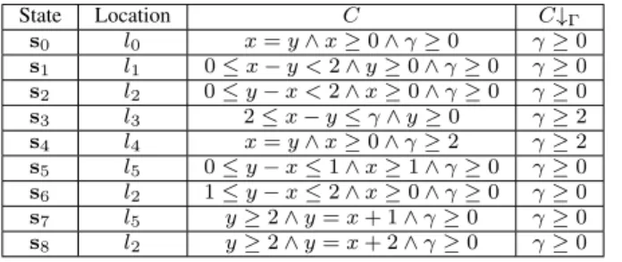
State Location 𝐶 𝐶↓Γ s0 𝑙0 𝑥 = 𝑦 ∧ 𝑥 ≥ 0 ∧ 𝛾 ≥ 0 𝛾 ≥ 0 s1 𝑙1 0 ≤ 𝑥 − 𝑦 < 2 ∧ 𝑦 ≥ 0 ∧ 𝛾 ≥ 0 𝛾 ≥ 0 s2 𝑙2 0 ≤ 𝑦 − 𝑥 < 2 ∧ 𝑥 ≥ 0 ∧ 𝛾 ≥ 0 𝛾 ≥ 0 s3 𝑙3 2 ≤ 𝑥 − 𝑦 ≤ 𝛾 ∧ 𝑦 ≥ 0 𝛾 ≥ 2 s4 𝑙4 𝑥 = 𝑦 ∧ 𝑥 ≥ 0 ∧ 𝛾 ≥ 2 𝛾 ≥ 2 s5 𝑙5 0 ≤ 𝑦 − 𝑥 ≤ 1 ∧ 𝑥 ≥ 1 ∧ 𝛾 ≥ 0 𝛾 ≥ 0 s6 𝑙2 1 ≤ 𝑦 − 𝑥 ≤ 2 ∧ 𝑥 ≥ 0 ∧ 𝛾 ≥ 0 𝛾 ≥ 0 s7 𝑙5 𝑦 ≥ 2 ∧ 𝑦 = 𝑥 + 1 ∧ 𝛾 ≥ 0 𝛾 ≥ 0 s8 𝑙2 𝑦 ≥ 2 ∧ 𝑦 = 𝑥 + 2 ∧ 𝛾 ≥ 0 𝛾 ≥ 0
Table II: Description of the states in 2b
∙ (s, 𝑎, Υ′) ∈ 𝑇 if there exists (𝑙, 𝑔, 𝑎, Υ) ∈ 𝕀 such that
for all 𝑙′ ∈ 𝐿, for all 𝜌 ⊆ 𝑋 such that Υ(𝑙′, 𝜌) > 0, 𝐶′=([𝐶 ∧ 𝑔]
𝜌)↗, and Υ′((𝑙′, 𝐶′)) = Υ(𝑙′, 𝜌).
Observe that, whenever a PIℙTA has no probabilistic choice, then the IMDP becomes a labeled transition system, and the symbolic semantics matches that of parametric timed automata. We refer to the symbolic semantics of𝒫ℐ𝒫 as the parametric probabilistic zone graph of𝒫ℐ𝒫.
Just as in parametric timed automata, the number of symbolic states in a PIℙTA can be infinite in general.
In parametric timed automata, the reachability condition is the projection onto the parameters of a parametric zone [17]. It is well-known that, given a symbolic run of a parametric timed automaton leading to a symbolic state (𝑙, 𝐶), there exists an equivalent concrete run iff𝛾 ∣= 𝐶↓Γ[18]. Since our definition of zones matches that of [18], this results extends to PIℙTAs in a straightforward manner.
Lemma 2. Let 𝒫ℐ𝒫 be a PIℙTA. Consider a run in
the parametric probabilistic zone graph of 𝒫ℐ𝒫 reaching state (𝑙, 𝐶). Let 𝑣 be a parameter valuation. Then, there exists an equivalent run in 𝑣(𝒫ℐ𝒫) iff 𝑣 ∣= 𝐶↓Γ.
By equivalent run, we mean (just as for parametric timed automata) an identical discrete structure (locations and edges).
Example 8. The parametric probabilistic zone graph of the
PIℙTA in 1b is the IMDP given in 2b. The symbolic states
s𝑖 = (𝑙𝑖, 𝐶𝑖) are expanded in II. In addition, we also give
the reachability condition of each state, i. e., the projection onto the parameters of the zone (𝐶↓Γ).
C. A Semi-Algorithm for Consistency-Synthesis for PIℙTAs Unlike for IℙTAs / IMDPs where inconsistent states can only be avoided by enforcing their incoming probabilities to 0, there are two ways of avoiding inconsistent states in PIℙTAs. Indeed, while imposing a 0 probability to all transitions going to inconsistent states is a safe choice, it is also possible to avoid inconsistent states by cleverly choosing parameter values such that the guards of transitions potentially going to these states are never satisfied.
The algorithm we propose for synthesizing parameter valuations ensuring consistency of a given PIℙTA is based
on the following observation: Since parameters only occur in transition guards, the choice of parameter values cannot interfere with the choice of probability distributions match-ing (or not) the specified intervals. That comes from the fact that, given a state s, all successors of this state via a given transition have the same parameter constraint (this would not hold with invariants). As a consequence, states that can be made unreachable through probabilistic choice can be made so regardless of the choice of parameter values.
2 is therefore constituted of two main parts. The first part (while loop – lines 5–9) is similar to 1 presented earlier. The main difference is that the loop from 2 does not entirely remove inconsistent states. Instead of systematically making locally inconsistent states unreachable whether this is allowed or not according to the specified intervals, this version marks inconsistent states (with marking function 𝜆) but only makes them unreachable when this is allowed, i. e., when replacing incoming transition probability intervals with [0, 0] does not make predecessor states inconsistent. If this is not the case, then the incoming transitions are left untouched but the predecessor states are marked as inconsistent with𝜆. If they can be made unreachable without creating new inconsistencies, then they will be made so in a later pass. Otherwise, locally inconsistent states will be “removed” using parameter valuations in the second loop.
Once the first loop is processed, the only locally incon-sistent states that remain are those that cannot be avoided using probabilities.
The second part (lines 18–22) consists in removing pa-rameter valuations that allow reaching locally inconsistent states in the resulting IMDP. In fact, instead of removing the inconsistent states, we remove their successors responsible for making a state inconsistent (lines 19–21). Also note that, due to the absence of invariants, all successors of a state through a given probability distribution have the same parameter constraint; it is hence sufficient to pick any of them. Recall from 2 that the parametric zone 𝐶↓Γ attached to a given symbolic state s = (𝑙, 𝐶) in the IMDP semantics of a given PIℙTA 𝒫ℐ𝒫 exactly represents the parameter valuations for which the states is reachable in the resulting semantics. As a consequence,s will be reachable in the IMDP semantics of the IℙTA resulting from a given parameter valuation iff this parameter valuation is in 𝐶↓Γ. Remark that the order in which locally inconsistent states are processed is not important. In fact, they can be all processed at once by removing all associated parameter zones. Proposition 1 (Termination). Let 𝒫ℐ𝒫 be a PIℙTA, and
letℐℳ be its parametric probabilistic zone graph. Assume ℐℳ is finite. Then the application of 2 to ℐℳ terminates. Proof: The first loop iterates on inconsistent states; at each iteration, one state is removed from Inc, and one or more states are added toInc. In addition, exactly one state is added to Passed; since a state in Passed can never be
Algorithm 2: Consistency of PIℙTAs
Input: IMDP ℐℳ (semantics of a PIℙTA 𝒫ℐ𝒫) Output: Constraint𝐾 guaranteeing consistency
1 LetInc be the set of locally inconsistent states in ℐℳ andPassed = ∅.
2 𝜆((𝑙, 𝐶)) = ∞ for all (𝑙, 𝐶) ∈ S ∖ Inc. 3 𝜆((𝑙, 𝐶)) = 0 for all (𝑙, 𝐶) ∈ Inc. 4 𝑛 = 0
5 whileInc ∕= ∅ do
6 Pick(𝑙, 𝐶) ∈ Inc s.t. 𝜆((𝑙, 𝐶)) ∕= ∞ is minimal 7 Passed = Passed ∪ {(𝑙, 𝐶)}.
8 Inc = Inc ∖ {(𝑙, 𝐶)}
9 for all transitions(s, 𝑎, 𝐼) such that s /∈ Passed and 𝐼((𝑙, 𝐶)) ∕= [0, 0] do 10 if0 ∈ 𝐼((𝑙, 𝐶)) and 𝐼[(𝑙, 𝐶)∣[0,0]] is consistent then 11 𝐼((𝑙, 𝐶)) ← [0, 0] 12 else 13 𝜆(s) = min(𝜆(s), 𝜆((𝑙, 𝐶)) + 1) 14 Inc ← Inc ∪ {s} 15 if𝜆(s0) = ∞ then 16 return⊤
17 Remove all unreachable states fromℐℳ 18 𝐾 ← ⊤
19 for all locally inconsistent transitions(𝑠, 𝑎, 𝐼) do 20 Pick a state(𝑙, 𝐶) such that 𝐼((𝑙, 𝐶)) ∕= [0, 0]
21 𝐾 ← 𝐾 ∖ 𝐶↓Γ
22 Remove inℐℳ and Inc all states (𝑙′, 𝐶′) such that 𝐶′↓Γ∩ 𝐾 = ⊥ (as well as transitions from and to
these states)
23 ifs0 has been removed then 24 return⊥
25 else
26 return𝐾
added again toInc, the first loop terminates.
The second loop iterates exactly once on each locally inconsistent transition, of which there is a finite number.
Proposition 2 (Correctness). Let 𝒫ℐ𝒫 be a PIℙTA, and
letℐℳ be its parametric probabilistic zone graph. Assume ℐℳ is finite. Let 𝐾 be the result of the application of 2 toℐℳ. Let 𝑣 ∣= 𝐾.
Then𝑣(𝒫ℐ𝒫) is consistent.
Proof (sketch): From 2 and the fact that any inconsis-tent state has been removed, and therefore valuations leading to inconsistent states are absent from𝐾.
Proposition 3 (Completeness). Let 𝒫ℐ𝒫 be a PIℙTA, and
letℐℳ be its parametric probabilistic zone graph. Assume ℐℳ is finite. Let 𝑣 be such that 𝑣(𝒫ℐ𝒫) is consistent. Let 𝐾 be the result of the application of 2 to ℐℳ.
Then 𝑣 ∣= 𝐾.
Proof (sketch): From 2 and the fact that only parameter valuations leading to inconsistent states (and for which no implementation of interval distribution can be set) are removed.
Remark 1. 2 is an algorithm: it always terminates, and
its result is sound and complete. However, it takes as input the parametric probabilistic zone graph of the PIℙTA, the computation of which may not terminate in general. Hence, our entire procedure (computation of the parametric probabilistic zone graph, and then application of 2) can be seen as a semi-algorithm: it may not terminate but, if it terminates, then its result is correct.
Example 9. Let us apply 2 to the PIℙTA 𝒫ℐ𝒫 given in 1b.
Recall that the parametric probabilistic zone graph of𝒫ℐ𝒫 is given in 2b, with the description of the states given in II. Initially, Inc = {s1} and 𝜆(s1) = 0 (and ∞ for other states). In the first while loop, setting to 0 the probability on the transition from s0 tos1 fails, because this does not satisfy the test “𝐼[(𝑙, 𝐶)∣[0,0]] is consistent” (10); indeed, the second probability leavings0 via action 𝑒1 can only be at most0.5. Hence, s0 becomes marked, and𝜆(s0) = 1.
Then, since the initial state is marked, we cannot conclude yet, and we enter the second phase. We have a single locally inconsistent transition, i. e., the one originating from s1. We pick arbitrarily s3 (picking s4 is identical), project its constraint ontoΓ, which yields 𝛾 ≥ 2 according to II, and perform the difference between 𝐾 and 𝛾 ≥ 2. This yields 𝐾 : 𝛾 < 2. We then remove states for which the parameter constraint is disjoint from𝐾, i. e., s3, s4. Sinces0 was not removed, we return𝐾 : 𝛾 < 2. Hence, for any parameter valuation𝑣 such that 𝛾 < 2, 𝑣(𝒫ℐ𝒫) is consistent.
V. CONCLUSION
In this work, we provided abstractions to reason on systems involving real-time constraints and probabilities: first, by allowing probabilities to range in some intervals, and, second, by allowing timing constants to be abstracted in the form of parameters. Without parameters, we proposed an approach to decide whether an interval probabilistic timed automaton is consistent, i. e., admits an implementation based on a simulation relation. When adding parameters, the mere existence of a parameter valuation yielding consistency is undecidable. We proposed however a semi-algorithm to synthesize valuations ensuring consistency.
Future works include the exhibition of subclasses of PIℙTAs for which exact synthesis can be achieved. In addition, we are interested in considering higher-level ab-stractions of probabilities, e. g., in the form of parameters instead of intervals with constant bounds.
REFERENCES
[1] R. Alur and D. L. Dill, “A theory of timed automata,”
Theoretical Computer Science, vol. 126, no. 2, pp. 183–235,
Apr. 1994.
[2] H. Gregersen and H. E. Jensen, “Formal design of reliable real time systems,” Master’s Thesis, Department of Mathematics and Computer Science, Aalborg University, 1995.
[3] M. Z. Kwiatkowska, G. Norman, R. Segala, and J. Sproston, “Automatic verification of real-time systems with discrete probability distributions,” Theoretical Computer Science, vol. 282, pp. 101–150, 2002.
[4] M. Z. Kwiatkowska, G. Norman, D. Parker, and J. Sproston, “Performance analysis of probabilistic timed automata using digital clocks,” Formal Methods in System Design, vol. 29, no. 1, pp. 33–78, 2006.
[5] R. Alur, T. A. Henzinger, and M. Y. Vardi, “Parametric real-time reasoning,” in Proceedings of the twenty-fifth annual
ACM symposium on Theory of computing, ser. STOC’93,
S. R. Kosaraju, D. S. Johnson, and A. Aggarwal, Eds. New York, NY, USA: ACM, 1993, pp. 592–601.
[6] ´E. Andr´e, L. Fribourg, and J. Sproston, “An extension of the inverse method to probabilistic timed automata,” Formal
Methods in System Design, no. 2, pp. 119–145, 2013.
[7] A. Jovanovi´c and M. Z. Kwiatkowska, “Parameter synthesis for probabilistic timed automata using stochastic game ab-stractions,” in Proceedings of the 8th International Workshop
on Reachability Problems (RP 2014), ser. Lecture Notes in
Computer Science, J. Ouaknine, I. Potapov, and J. Worrell, Eds., vol. 8762. Springer, 2014, pp. 176–189.
[8] B. Jonsson and K. Larsen, “Specification and refinement of probabilistic processes,” in LICS. IEEE Computer, 1991, pp. 266–277.
[9] B. Delahaye, K. G. Larsen, A. Legay, M. L. Pedersen, and A. Wasowski, “Consistency and refinement for interval markov chains,” J. Log. Algebr. Program., vol. 81, no. 3, pp. 209–226, 2012.
[10] J. Bengtsson and W. Yi, “Timed automata: Semantics, al-gorithms and tools,” in Lectures on Concurrency and Petri
Nets, Advances in Petri Nets, ser. Lecture Notes in Computer
Science, J. Desel, W. Reisig, and G. Rozenberg, Eds., vol. 3098. Springer, 2003, pp. 87–124.
[11] B. Delahaye, “Consistency for parametric interval markov chains,” in 2nd International Workshop on Synthesis of
Com-plex Parameters, SynCoP 2015, April 11, 2015, London,
United Kingdom, ser. OASICS, vol. 44. Schloss Dagstuhl
-Leibniz-Zentrum fuer Informatik, 2015, pp. 17–32.
[12] B. Delahaye, D. Lime, and L. Petrucci, “Parameter synthesis for parametric interval markov chains,” in Verification, Model
Checking, and Abstract Interpretation - 17th International Conference, VMCAI 2016, St. Petersburg, FL, USA, January 17-19, 2016. Proceedings, ser. Lecture Notes in Computer
Science, vol. 9583. Springer, 2016, pp. 372–390.
[13] G. Behrmann, P. Bouyer, K. G. Larsen, and R. Pel´anek, “Lower and upper bounds in zone-based abstractions of timed automata,” International Journal on Software Tools for
Technology Transfer, vol. 8, no. 3, pp. 204–215, 2006.
[14] ´E. Andr´e, “What’s decidable about parametric timed au-tomata?” in Proceedings of the 4th International Workshop on
Formal Techniques for Safety-Critical Systems (FTSCS’15),
ser. Communications in Computer and Information Science, C. Artho and P. C. ¨Olveczky, Eds., vol. 596. Springer, 2016, pp. 1–17.
[15] N. Beneˇs, P. Bezdˇek, K. G. Larsen, and J. Srba, “Language emptiness of continuous-time parametric timed automata,” in ICALP, Part II, ser. Lecture Notes in Computer Science, M. M. Halld´orsson, K. Iwama, N. Kobayashi, and B. Speck-mann, Eds., vol. 9135. Springer, Jul. 2015, pp. 69–81. [16] ´E. Andr´e, Th. Chatain, E. Encrenaz, and L. Fribourg, “An
inverse method for parametric timed automata,” International
Journal of Foundations of Computer Science, vol. 20, no. 5,
pp. 819–836, 2009.
[17] A. Jovanovi´c, D. Lime, and O. H. Roux, “Integer parameter synthesis for timed automata,” IEEE Transactions on Software
Engineering, vol. 41, no. 5, pp. 445–461, 2015.
[18] T. Hune, J. Romijn, M. Stoelinga, and F. W. Vaandrager, “Lin-ear parametric model checking of timed automata,” Journal of
Logic and Algebraic Programming, vol. 52-53, pp. 183–220,