Pattern-based constraint satisfaction and logic puzzles

(1)

HAL Id: hal-00808151

https://hal.archives-ouvertes.fr/hal-00808151

Submitted on 5 Apr 2013

HAL is a multi-disciplinary open access

archive for the deposit and dissemination of

sci-entific research documents, whether they are

pub-lished or not. The documents may come from

teaching and research institutions in France or

abroad, or from public or private research centers.

L’archive ouverte pluridisciplinaire HAL, est

destinée au dépôt et à la diffusion de documents

scientifiques de niveau recherche, publiés ou non,

émanant des établissements d’enseignement et de

recherche français ou étrangers, des laboratoires

publics ou privés.

Pattern-based constraint satisfaction and logic puzzles

Denis Berthier

To cite this version:

Denis Berthier. Pattern-based constraint satisfaction and logic puzzles. Lulu.com, pp.480, 2012,

978-1-291-20339-4. �hal-00808151�

(2)

Pattern-Based Constraint Satisfaction

and Logic Puzzles

Denis Berthier

Institut Mines Télécom

This is the full text of the book published in print form by Lulu

Publishers (Nov. 2012, ISBN 978-1-291-20339-4).

(3)

(4)

Pattern-Based Constraint Satisfaction

and Logic Puzzles

(5)

(6)

Denis Berthier

Pattern-Based Constraint Satisfaction

and Logic Puzzles

(7)

Books by Denis Berthier:

Le Savoir et l’Ordinateur, Editions L’Harmattan, Paris, November 2002. Méditations sur le Réel et le Virtuel, Editions L’Harmattan, Paris, May 2004. The Hidden Logic of Sudoku (First Edition), Lulu.com, May 2007.

The Hidden Logic of Sudoku (Second Edition), Lulu.com, November 2007. Constraint Resolution Theories, Lulu.com, November 2011.

Keywords: Constraint Satisfaction, Artificial Intelligence, Constructive Logic, Logic Puzzles, Sudoku, Futoshiki, Kakuro, Numbrix®_{, Hidato}®_.

This work is subject to copyright. All rights are reserved. This work may not be translated or copied in whole or in part without the prior written permission of the copyright owner, except for brief excerpts in connection with reviews or scholarly analysis. Use in connection with any form of information storage or retrieval, electronic adaptation, computer software, or by similar or dissimilar methods now known or hereafter developed, is forbidden.

9 8 7 6 5 4 3 2 1

Dépôt légal: Novembre 2012

(8)

Foreword

Motivations for the approach of the present book

Since the 1970s, when it was identified as a class of problems with its own specificities, Constraint Satisfaction has quickly evolved into a major area of Artificial Intelligence (AI). Two broad families of very efficient algorithms (with many freely available implementations) have become widely used for solving its instances: general purpose structured search of the “problem space” (e.g. depth-first, breadth-first) and more specialised “constraint propagation” (that must generally be combined with search according to various recipes).

One may therefore wonder why they would use the computationally much harder techniques inherent in the approach introduced in the present book. It should be clear from the start that there is no reason at all if speed is the first or only criterion, as may legitimately be the case in such a typical Constraint Satisfaction Problem (CSP) as scene labelling.

But, instead of just wanting a final result obtained by any available and/or efficient method, one can easily imagine additional requirements of various types and one may thus be interested in how the solution was reached, i.e. by the resolution path. Whatever meaning is associated with the quoted words below, there are several inter-related families of requirements one can consider:

– the solution must be built by “constructive” methods, with no “guessing”; – the solution must be obtained by “pure logic”;

– the solution must be “pattern-based”, “rule-based”; – the solution must be “understandable”, “explainable”; – the solution must be the “simplest” one.

Vague as they may be, such requirements are quite natural for logic puzzles and in many other conceivable situations, e.g. when one wants to ask explanations about the solution or parts of it.

Starting from the above vague requirements, Part I of this book will elaborate a formal interpretation of the first three, leading to a very general, pattern-based resolution paradigm belonging to the classical “progressive domain restriction” family and resting on the notions of a resolution rule and a resolution theory.

(13)

Then, in relation with the last purpose of finding the “simplest” solution, it will introduce ideas that, if read in an algorithmic perspective, should be considered as defining a new kind of search, “simplest-first search” – indeed various versions of it based on different notions of logical simplicity. However, instead of such an algorithmic view (or at least before it), a pure logic one will systematically be adopted, because:

– it will be consistent with the previous purposes,

– it will convey clear non-ambiguous semantics (and it will therefore include a unique complete specification for possibly multiple types of implementation),

– it will allow a deeper understanding of the general idea of “simplest-first search”, in particular of how there can be various underlying concrete notions of logical simplicity and how these have to be defined by different kinds of resolution rules associated with different types of chain patterns. At this point, it may be useful to notice that the classical structured search algorithms are not compatible with pure logic definitions (as will be explained in the text).

Simplest-first search and the rating of instances

In this context, there will appear the question of rating and/or classifying the instances of a (fixed size) CSP according to their “difficulty”. This is a much more difficult topic than just solving them. The families of resolution rules introduced in this book (by order of increasing complexity) will go by couples (corresponding to two kinds of chains with no OR-branching but with different linking properties, namely T-whips and T-braids); for each couple, there will be two ratings, defined in pure logic ways:

– one based on T-braids, allowing a smooth theoretical development and having good abstract computational properties; we shall devote much time to prove the confluence property of all the braid and T-braid resolution theories, because it justifies a “simplest-first” resolution strategy (and the associated “simplest-first search” algorithms that may implement it) and it allows to find the “simplest” resolution path and the corresponding rating by trying only one path;

– one based on T-whips, providing in practice an easier to compute good approximation of the first when it is combined with the “simplest-first” strategy. (The quality of the approximation can be studied in detail and precisely quantified in the Sudoku case, but it will also appear in intuitive form in all our other examples.)

We shall explain in which restricted sense all these ratings are compatible. But we shall also show that each of them corresponds to a different legitimate pure logic view of simplicity.

In chapter 11, we shall analyse the scope of the previously defined resolution rules in terms of a search procedure with no guessing, Trial-and-Error (T&E), and of

(14)

Foreword 11

the depth of T&E necessary to solve an instance. There are universal ratings, respectively the B and the BB ratings, for instances in T&E(1) and T&E(2) (i.e. requiring no more than one or two levels of Trial-and-Error). Universality must be understood in the sense that they assign a finite rating to all of these instances, but not in the sense that they could provide a unique notion of simplicity. For instances beyond T&E(2), it is questionable whether a “pure logic” solution, with all the complex and boring steps that it would involve, would be of any interest; moreover, it appears that there may be many different incompatible notions of “simplest”; in chapter 12, we shall introduce the notion of a pattern of proof and, based on it, we shall re-assess our initial requirements. The main purpose is to provide hints about the scope of practical validity of our approach.

Examples from logic puzzles

Mainly because they can be described shortly and they are easy to understand with no previous knowledge, all the examples dealt with in this book will be logic puzzles: Latin Squares, Sudoku, N-Queens…, with a special status granted to Sudoku for reasons that will be explained in the Introduction. But they have been selected in such a way that they make us tackle very different types of constraints, so that this choice should not suggest a lack of generality in our approach: transitive constraints in Futoshiki, non-binary arithmetic constraints in Kakuro, topological and geometric constraints in Map colouring or path finding (Numbrix®_{and Hidato}®_).

In several places, we shall even give results that are only valid for 9×9 Sudoku (e.g. the unbiased whip classification results of minimal instances in chapter 6 and the analysis of extreme instances in chapter 11), for the purpose of illustrating with precise quantitative data questions that cannot yet be tackled with such detail in other CSPs and that call for further studies, such as:

– the difficulty (much beyond what one may imagine) of finding uncorrelated unbiased samples of minimal instances of a CSP, a pre-requisite for any statistical analysis; the way we present it shows that it is likely to appear in many CSPs; the final chapters on various other CSPs show that this is indeed true for them; (a related well known problem is that of finding the hardest instances of a CSP);

– the surprisingly high resolution power of short whips for instances in T&E(1); – the concrete application of various classification principles to the extreme instances.

The “Hidden Logic of Sudoku” heritage [mainly for the readers of HLS]

The origins of the work reported in this book can be traced back to my choice of Sudoku as a topic of practical classes for an introductory course in Artificial Intelligence (AI) and Rule-Based Systems in early 2006. As I was formalising for

(15)

myself the simplest classical techniques (Subset rules, xy-chains) before submitting them as exercises to my students, I had two ideas that kept me interested in this game longer than I had first expected: logical symmetries between three well-known types of Subset rules (Naked, Hidden and Super-Hidden, the last of which are commonly known as “Fish”) and a simple non-reversible extension (xyt-chains) of the well-known reversible xy-chains. As time passed, the short article I had planned to write grew to the size of a 430-page book: The Hidden Logic of Sudoku – HLS in the sequel (first edition, HLS1, May 2007; second edition, HLS2, November 2007).

The present book inherits many of the ideas I first introduced in HLS but it extends them to any finite CSP. Based on the classical idea of candidate elimination, HLS provided a clear logical status for the notion of a candidate (which does not pertain to the original problem formulation) and it introduced the notions of a resolution rule and a resolution theory. All the concepts were strictly formalised in Predicate Logic (FOL) – more precisely in Multi Sorted First Order Logic (MS-FOL) – which (surprisingly) was a new idea: previously, all the books and Web forums had always considered that Propositional Logic was enough. Indeed, HLS had to make a further step, because intuitionistic (or, equivalently, constructive) logic is necessary for the proper formalisation of the notion of a candidate.

Notwithstanding the more general formulation, the “pattern-based” conceptual framework developed in this book is very close to that of HLS. From the start, the framework of HLS was intended as a formalisation of what had always been looked for when it was said that a “pure logic solution” was wanted. The basic concepts appearing in the resolution rules introduced in HLS were grounded in the most elementary notions used to propose or solve a puzzle (numbers, rows, columns, blocks, …); the more elaborate ones (the various types of chain patterns) were progressively introduced and strictly defined from the basic ones. Because the concepts of a candidate and of a link between two candidates were enough to formulate most of the resolution rules, extending them to any CSP was almost straightforward. The additional requirement that appeared in HLS in relation with the idea of rating, that of finding the simplest resolution path, is also tackled here according to the same general principles as in HLS.

On the practical puzzle solving side, HLS1 introduced new resolution rules, based on natural generalisations of the famous xy-chains, such as xyt-, xyz- and zyzt- chains; contrary to those proposed in the current Sudoku literature, these were not based on “Subsets” (or almost locked sets – “ALS”) and most of these chains were not “reversible”; the systematic clarification and exploitation of all the generalised symmetries of the game and the combination of my first two initial ideas had also led me to the “hidden” counterparts of the previous chains (hxy-, hxyt- hxyzt- chains). Later, I found further generalisations (nrczt- chains and lassoes), pushing the idea of supersymmetry to its maximal extent and allowing to solve

(16)

Foreword 13

almost any puzzle with short chain patterns. Giving a more systematic presentation of these new “3D” chain rules was the main reason for the second edition (HLS2).

Still later, I introduced (on Sudoku forums) other generalisations (that, in the simplified terminology of the present book and in a formulation meaningful for any CSP, will appear as whips, braids, g-whips, Sp-whips, Wp-whips, …). These may

have justified a third edition of HLS, but I have just added a few pages to my HLS website instead – concentrating my work on another type of generalisation.

It appeared to me that most of what I had done for Sudoku could be generalised to any finite CSP [Berthier 2008a, 2008b, 2009]. But, once more, as I found further generalisations and as the analysis of additional CSPs with different characteristics was necessary to guarantee that my definitions were not too restrictive, the normal size of journal articles did not fit the purposes of a clear and systematic exposition; this is how this work grew into a new book, “Constraint Resolution Theories” (CRT, November 2011).

As for the resolution rules themselves, whereas HLS proceeded by successive generalisations of well-known elementary rules for Sudoku into more complex ones, in CRT and in the present book, we start (in Part II) from powerful rules meaningful in any CSP (whips, in chapter 5) equivalent (in the Sudoku case) to those that were only reached at the end of HLS2 (nrczt- chains and lassoes).

As a result, in this book, patterns such as Subsets, with much less resolution power than whips of same size and with more complex definitions in the general CSP than in Sudoku, come after bivalue-chains, whips and braids, and also after their “grouped” versions, g-whips and g-braids. Moreover, Subsets are introduced here with purposes very different from those in HLS:

1) providing them with a definition meaningful in any CSP (in particular, independent of any underlying grid structure);

2) showing that whips subsume most cases of Subsets in any CSP;

3) illustrating by Sudoku examples how, in rare cases, Subset rules can nevertheless simplify the resolution paths obtained with whips;

4) defining in any CSP a “grouped” version of Subsets, g-Subsets; surprisingly, in the Sudoku case, g-Subsets do not lead to new rules, but they give a new perspective of the well-known Franken and Mutant Fish; this could be useful for the purposes of classifying these patterns (which has always been a very obscure topic);

5) showing that, in any CSP, the basic principles according to which whips are built can be generalised to allow the insertion of Subsets into them (obtaining Sp-whips),

thus extending the resolution power of whips towards the exceptionally hard instances.

(17)

What is new with respect to “Constraint Resolution Theories” [mainly for the readers of CRT]

This book can be considered as the second, revised and largely extended edition of Constraint Resolution Theories (CRT). Following a colleague’s advice, we changed the title (which seemed too technical) so that it includes the “Constraint Satisfaction” key phrase referring to its global domain; “Pattern-Based” was then a natural choice for qualifying our approach, while the explicit reference to “Logic Puzzles” became almost necessary with the addition of all the examples in part IV to the already existing Sudoku content. Apart from this cosmetic change, there are three different degrees of newness with respect to CRT, in increasing magnitude.

Firstly, this book corrects a few typos and errors that remained in CRT in spite of careful re-readings; in several places, it also marginally improves or completes the wording and it adds a few remarks or comments; moreover:

– z-chains are no longer included in the analysis of loops in sections 5.8.1 to 5.8.3; instead, the obvious and simpler fact that z-whips subsume z-chains with a global loop is mentioned;

– an unnecessary restriction in the definition of a g-label (section 7.1.1.1) has been eliminated, without modifying the notion of a g-link; this leaves unchanged the definitions of a g-candidate and of predicate “g-linked” (relating a g-candidate and a candidate); as before, these two definitions refer to the full underlying g-label and label (this is why the restriction was unnecessary); nothing else had to be changed in chapter 7 or in any place where g-labels are dealt with; in particular, this does not change the sets of g-labels of the various examples already tackled by CRT; however, the restriction made it impossible to apply the initial definition given in CRT to g-labels in Futoshiki (see chapter 14);

– the “saturation” or “local maximality” condition in the definition of a g-label has been broadened for an easier applicability to new examples; it has also been isolated by splitting the initial definition into two parts; as it was there only for efficiency purposes, but it had no impact on theoretical analyses, this entails no other changes; however, the efficiency purposes should not be underestimated: section 15.5 shows how essential this condition is in practice in Kakuro;

– section 11.4 of CRT (bi-whips, bi-braids, W*-whips and B*-braids) has been significantly reworded, corrected and extended, giving rise to a new chapter of its own (chapter 12);

– a section (17.4) describing our general pattern-based CSP-Rules solver, used for all the examples presented in this book, has been introduced.

Secondly, this book adds a few new results, mainly to the W-whip and B-braid patterns and/or to the Sudoku CSP case study. The following list is not exhaustive:

(18)

Foreword 15

– very instructive whip[2] examples are given in section 8.8.1; they are the key for understanding why whips can be more powerful than Subsets of same size;

– an example of a non-whip braid[3] in Sudoku is given in section 5.10.5; – a new graphico-symbolic representation of W-whips is introduced in section 11.2.9, based on the analogy between whips and Subsets;

– the most recent collections of extreme puzzles, harder than most of those already considered in CRT, published in the meantime by various puzzle creators, are analysed and their B?B classifications are given in section 11.4; these new

results show that a few puzzles (we have found only three in these collections) require B7-braids and they provide very strong support to our old conjecture that all

the 9×9 Sudoku puzzles can be solved by T&E(2) and to our new one that they can all be solved by B7-braids;

– occasionally, larger sized Sudoku grids are considered; this allows in particular to show that the universal solvability by T&E(2) is not true for them.

Thirdly and most importantly, chapter 12 and part IV about modelling various logic puzzles are almost completely new; in particular:

– chapter 12, revolving around the notion of a pattern of proof, shows that our initial simplicity and understandability requirements may be at variance for instances beyond T&E(1) or gT&E(1); it discusses various options for their interpretation, such as B*-braid solutions; it shows that a pure logic approach is still possible in theory, although the computational complexity may be much higher, depending on which patterns of proof one is ready to accept;

– chapter 13, via an illustrative example (the sk-loop in Sudoku), tackles general questions about modelling resolution rules; these arise when one wants to formalise new (possibly application-specific) techniques; although part of the material in it has been available for several years on the Sudoku part of our website in a rather technical form, subtle changes (making the presentation much simpler and slightly more general) appear here for the first time;

– chapter 14 on transitive constraints and the Futoshiki CSP concretely shows how the general concepts and resolution rules defined in this book can be applied to a CSP with significantly different types of constraints (inequalities) than the symmetric ones considered in the LatinSquare, Sudoku and N-Queens examples; it also shows that the few known, apparently application-specific, resolution rules of Futoshiki (ascending chains, hills and valleys) are special cases of these general rules; finally, it indicates how our controlled-bias approach to puzzle generation, at the basis of any unbiased statistical results, can be adapted to it in a straightforward way;

– chapter 15 on non-binary arithmetic constraints and the Kakuro CSP may be the most important one among our non-Sudoku examples, as it shows that the binary

(19)

constraints restriction of our approach can be relaxed not only in theory but also in practice and that non-binary constraints can be efficiently managed in application-specifc ways (better than by relying on the standard general replacement method);

– chapter 16 deals with some topological and geometric constraints associated with map colouring and path finding (in Numbrix®_{and Hidato}®_{); together with}

chapters 14 and 15, it confirms that our generalisations from Sudoku to the general CSP work concretely – a point in which CRT was partially lacking.

(20)

1. Introduction

1.1. The general Constraint Satisfaction Problem (CSP)

Many real world problems, such as resource allocation, temporal reasoning, activity scheduling, scene labelling…, naturally appear as Constraint Satisfaction Problems (CSP) [Guesguen et al. 1992, Tsang 1993]. Many theoretical problems and many logic games are also natural examples of CSPs: graph colouring, graph matching, cryptarithmetic, N-Queens, Latin Squares, Sudoku and its innumerable variants, Futoshiki, Kakuro and many other logic games (or logic puzzles).

In the past decades, the study of such problems has evolved into a main sub-area of Artificial Intelligence (AI) with its own specialised techniques. Research has concentrated on finding efficient algorithms, which was a necessity for dealing with large scale applications. As a result, one aspect of the problem has been almost completely overlooked: producing readable solutions. This aspect will be the main topic of the present book.

1.1.1. Statement of the Constraint Satisfaction Problem

A CSP is defined by:

– a set of variables X1, X2, … Xn, the “CSP variables”, each with values in a

given domain Dom(X1), Dom(X2), …, Dom(Xn),

– a set of constraints (i.e. of relations) these variables must satisfy.

The problem consists of assigning a value from its domain to each of these variables, such that these values satisfy all the constraints. Later (in Chapter 3), we shall show that a CSP can easily be re-written as a theory in First Order Logic.

As in many studies of CSPs, all the CSPs we shall consider in this book will be finite, i.e. the number of variables, each of their domains and the number of constraints will all be finite. When we write “CSP”, it should therefore always be read as “finite CSP”.

Also, we shall consider only CSPs with binary constraints. One can always tackle unary constraints by an appropriate choice of the domains. And, for k > 2, a k-ary constraint between a subset of k variables (Xn1, .., Xnk) can always be replaced

(21)

representing the original k-ary constraint; although this new variable has a large domain and this may be a very inefficient way of dealing with the given k-ary constraint, this is a very standard approach (for details, see [Tsang 1993]). With the Kakuro CSP, chapter 15 will show an example of how this can be done in practice, using application specific techniques more efficient than the general method.

Moreover, a binary CSP can always be represented as a (generally large) labelled undirected graph: a node (or vertex) of this graph, called a label, is a couple < CSP variable, possible value for it > (or, in our approach, an equivalence class of such couples); given two nodes in this graph, each binary constraint not satisfied by this pair of labels (including the “strong” constraints induced by CSP variables, i.e. all the contradictions between different values for the same CSP variable) gives rise to an arc (or edge) between them, labelled by the name of the constraint and representing it. We shall call this graph the CSP graph. (Notice that this is different from what is usually called the constraint graph.) The CSP graph expresses all the direct contradictions between any two labels (whereas the constraint graph usually considered in the CSP literature expresses their compatibilities).

1.1.2. The Sudoku example

As explained in the foreword, Sudoku has been at the origin of our work on CSPs. In this book, we shall keep it as our main example for illustrating the techniques we introduce, even though we shall also deal with other CSPs in order to palliate its specificities (for other detailed examples, see chapters 14 to 16).

Let us start with the usual formulation of the problem (with its own, self-explanatory vocabulary in italics): given a 9×9 grid, partially filled with numbers from 1 to 9 (the givens of the problem, also called the clues or the entries), complete it with numbers from 1 to 9 in such a way that in each of the nine rows, in each of the nine columns and in each of the nine disjoint blocks of 3×3 contiguous cells, the following property holds:

– there is at most one occurrence of each of these numbers.

Although this defining condition could be replaced by either of the following two, which are obviously equivalent to it, we shall stick to the first formulation, for reasons that will appear later:

– there is at least one occurrence of each of these numbers, – there is exactly one occurrence of each of these numbers.

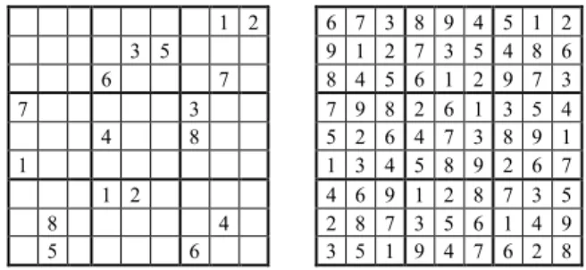
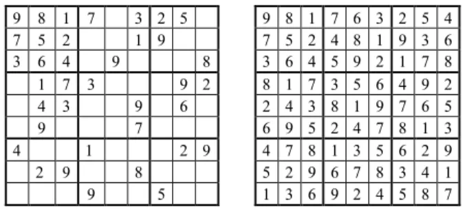
Figure 1.1 shows the standard presentations of a problem grid (also called a Sudoku puzzle) and of a solution grid (also called a complete Sudoku grid).

Since rows, columns and blocks play similar roles in the defining constraints, they will naturally appear to do so in many other places and a word that makes no

(22)

1. Introduction 19

difference between them is widely used in the Sudoku world: a unit is either a row or a column or a block. And one says that two cells share a unit, or that they see each other, if they are different and they are either in the same row or in the same column or in the same block (where “or” is non exclusive). We shall also say that these two cells are linked. It should be noticed that this (symmetric) relation between two different cells, whichever of the three equivalent names it is given, does not depend on the content of these cells but only on their place in the grid; it is therefore a straightforward and quasi physical notion.

1 2 6 7 3 8 9 4 5 1 2 3 5 9 1 2 7 3 5 4 8 6 6 7 8 4 5 6 1 2 9 7 3 7 3 7 9 8 2 6 1 3 5 4 4 8 5 2 6 4 7 3 8 9 1 1 1 3 4 5 8 9 2 6 7 1 2 4 6 9 1 2 8 7 3 5 8 4 2 8 7 3 5 6 1 4 9 5 6 3 5 1 9 4 7 6 2 8

Figure 1.1. A puzzle (Royle17#3) and its solution

As appears from the definition, a Sudoku grid is a special case of a Latin Square. Latin Squares must satisfy the same constraints as Sudoku, except the condition on blocks. Following HLS1, the logical relationship between the two theories will be fully clarified in chapters 3 and 4.

What we need now is to see how the above natural language formulation of the Sudoku problem can be re-written as a CSP. In Chapter 2, the essential question of modelling in general and its practical implications on how to deal with a CSP will be raised and we shall see that the following formalisation is neither the only one nor the best one. But, for the time being, we only want to write the most straightforward one.

For each row r and each column c, introduce a variable Xrc with domain the set

of digits {1, 2, 3, 4, 5, 6, 7, 8, 9}. Then the general Sudoku problem can be expressed as a CSP for these variables, with the following set of (binary) constraints:

Xrc ≠ Xr’c’ for all the pairs {rc, r’c’} such that the cells rc and r’c’ share a unit,

and a particular puzzle will add to these binary constraints the set of unary constraints fixing the values of the Xrc variables corresponding to the givens.

Notice that the natural language phrase “complete the grid” in the original formulation has naturally been understood as “assign one and only one value to each

(23)

of the cells” – which has then been translated into “assign a value to each of the Xrc

variables” in the CSP formulation.

1.2. Paradigms of resolution

A CSP states the constraints a solution must satisfy, i.e. it says what is desired. But it does not say anything about how a solution can be obtained; this is the job of resolution methods, the choice of which will depend on the various purposes one may have in addition to merely finding a solution. A particular class of resolution methods, based on resolution rules, will be the main topic of this book.

1.2.1. Various purposes and methods

If one’s only goal is to get a solution by any available means, very efficient general-purpose algorithms have been known for a long time [Kumar 1992, Tsang 1993]; they guarantee that they will either find one solution or all the solutions (according to what is desired) or find a contradiction in the givens; they have lots of more recent variants and refinements. Most of these algorithms involve the combination of two very different techniques: some direct propagation of constraints between variables (in order to progressively reduce their sets of possible values) and some kind of structured search with “backtracking” (depth-first, breadth-first, …, possibly with some forms of look-ahead); they consist of trying (recursively if necessary) a value for a variable and propagating (based on the constraints) the consequences of this tentative choice as restrictions on other variables; eventually, either a solution or a contradiction will be reached; the latter case allows to conclude that this value (or this combination of values simultaneously tried in the recursive case) is impossible and it restricts the possibilities for this (subset of) variables(s).

But, in some cases, such blind search is not possible for practical reasons (e.g. one is not in a simulator but in real life) or not allowed (for a priori theoretical or æsthetic reasons), or one wants to simulate human behaviour, or one wants to “understand” or to be able to “explain” each step of the resolution process (as is generally the case with logic puzzles), or one wants a “constructive” solution (with no “guessing”) or one wants a “pure logic” or a “pattern-based” or a “rule-based” or the “simplest” solution, whatever meaning they associate with the quoted words.

Contrary to the current CSP literature, this book will only deal with the latter cases and more attention will be paid to the resolution path than to the final solution itself. Indeed, it can also be considered as an informal reflection on how notions such as “no guessing”, “a constructive solution”, “a pure logic solution”, “a pattern-based solution”, “an understandable proof of the solution”, “an explanation of the solution” and “the simplest solution” can be defined (but we shall only be able to say more on this topic in the retrospective “final remarks” chapter). It does not mean

(24)

1. Introduction 21

that efficiency questions are not relevant to our approach, but they are not our primary goal, they are conditioned by such higher-level requirements. Without these additional requirements, there is no reason to use techniques computationally much harder (probably exponentially much harder) than the general-purpose algorithms.

In such situations, it is convenient to introduce the notion of a candidate, i.e. of a “still possible” value for a variable. As this intuitive notion does not pertain to the CSP itself, it must first be given a clear definition and a logical status. When this is done (in chapter 4), one can define the concepts of a resolution rule (a logical formula in the “condition ⇒ action” form, which says what to do in some factual, observable situation described by the condition pattern), a resolution theory (a set of such rules), a resolution strategy (a particular way of using the rules in a resolution theory). One can then study the relationship between the original CSP and several of its resolution theories. One can also introduce several properties a resolution theory can have, such as confluence and completeness (contrary to general purpose algorithms, a resolution theory cannot in general solve all the instances of a given CSP; evaluating its scope is thus a new topic in its own; one can also study its statistical resolution power in specific CSP cases).

This “rule-based” or “pattern-based” approach was first introduced in HLS1, in the limited context of Sudoku. It is the purpose of this book to show that it is indeed very general and chapters 14 to 16 will concretely show that it does apply to the very different types of constraints appearing in Futoshiki, Kakuro and map colouring, but let us first illustrate how these ideas work for Sudoku.

1.2.2. Candidates and candidate elimination in Sudoku

The process of solving a Sudoku puzzle “by hand” is generally initialised by defining the “candidates” for each cell. For later formalisation, one must be careful with this notion: if one analyses the natural way of using it, it appears that, at any stage of the resolution process, a candidate for a cell is a number that has not yet been explicitly proven to be an impossible value for this cell.

Usually, candidates for a cell are displayed in the grid as smaller and/or clearer digits in this cell (as in Figure 1.2). Similarly, at any stage, a decided value is a number that has been explicitly proven to be the only possible value for this cell; it is written in big fonts, like the givens.

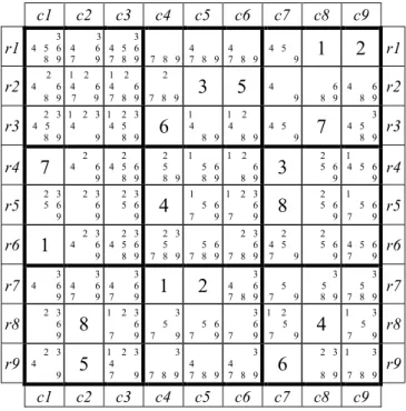
At the start of the game, one possibility is to consider that any cell with no input value admits all the numbers from 1 to 9 as candidates – but more subtle initialisations are possible (e.g. as shown in Figure 1.2) and a slightly different, more symmetric, view of candidates can be introduced (see chapter 2).

Then, according to the formalisation introduced in HLS1, a resolution process that corresponds to the vague requirement of a “pure logic” solution is a sequence of

(25)

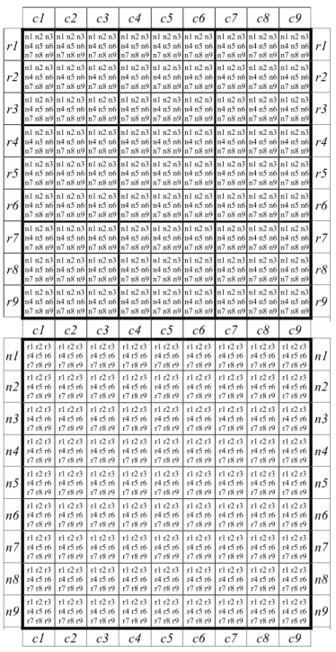
steps consisting of repeatedly applying “resolution rules” of the general condition-action type: if some pattern – i.e. configuration of cells, possible cell-values, links, decided values, candidates and non-candidates – defined by the condition part of the rule, is effectively present in the grid, then carry out the action(s) specified by the action part of the rule. Notice that any such pattern always has a purely “physical”, invariant part (which may be called its “physical” or “structural” support), defined by conditions on possible cell-values and on links between them, and an additional part, related to the actual presence/absence of decided values and/or candidates in these cells in the current situation. (Again, this will be generalised in chapter 2 with the four “2D” views.)

c1 c2 c3 c4 c5 c6 c7 c8 c9 r1 3 4 5 6 8 9 3 4 6 7 9 3 4 5 6 7 8 9 7 8 9 4 7 8 9 4 7 8 9 4 5 9

1

2

r1 r2 4 6 2 8 9 1 2 4 6 7 9 1 2 4 6 7 8 9 2 7 8 9

3

5

4 9 6 8 9 4 6 8 9 r2 r3 4 5 2 3 8 9 1 2 3 4 9 1 2 3 4 5 8 9

6

1 4 8 9 1 2 4 8 9 4 5 9

7

3 4 5 8 9 r3 r4

7

2 4 6 9 2 4 5 6 8 9 2 5 8 9 1 5 6 8 9 1 2 6 8 9

3

2 5 6 9 1 4 5 6 9 r4 r5 2 3 5 6 9 2 3 6 9 2 3 5 6 9

4

1 5 6 7 9 1 2 3 6 7 9

8

2 5 6 9 1 5 6 7 9 r5 r6

1

2 3 4 6 9 2 3 4 5 6 8 9 2 3 5 7 8 9 5 6 7 8 9 2 3 6 7 8 9 2 4 5 7 9 2 5 6 9 4 5 6 7 9 r6 r7 3 4 6 9 3 4 6 7 9 3 4 6 7 9

1

2

3 4 6 7 8 9 5 7 9 3 5 8 9 3 5 7 8 9 r7 r8 2 3 6 9

8

1 2 3 6 7 9 3 5 7 9 5 6 7 9 3 6 7 9 1 2 5 7 9

4

1 3 5 7 9 r8 r9 2 3 4 9

5

1 2 3 4 7 9 3 7 8 9 4 7 8 9 3 4 7 8 9

6

2 3 8 9 1 3 7 8 9 r9 c1 c2 c3 c4 c5 c6 c7 c8 c9

Figure 1.2. Grid Royle17#3 of Figure 1.1, with the candidates remaining after the elementary

constraints for the givens have been propagated

Depending on the type of their action part, such resolution rules can be classified into two categories (assertion type and elimination type):

– either they assert a decided value for a cell (e.g. the Single rule: if it is proven that there is only one possibility left for it); there are very few such assertion rules;

– or they eliminate some candidate(s) (which we call the target(s) of the pattern); as appears from a quick browsing of the available literature, almost all the

(26)

1. Introduction 23

classical Sudoku resolution rules are of this type (and, apart from Singles, the few rules that seem to be of the assertion type can be reduced to elimination rules); they express elaborated forms of constraints propagation; their general form is: if such pattern is present, then it is impossible for some number(s) to be in some cell(s) and the target candidates must therefore be deleted; for the general CSP also, all the rules we shall meet in this book, apart from Singles, will be of the elimination type.

The interpretation of the above resolution rules, whatever their type, should be clear: none of them claims that there is a solution with such value asserted or such candidate deleted. Rather, it must be interpreted as saying: “from the current situation it can be asserted that any solution, if there is any, must satisfy the conclusion of this rule”.

From both theoretical and practical points of view, it is also important to notice that, as one proceeds with resolution, candidates form a monotone decreasing set and decided values form a monotone increasing set. Whereas the notion of a candidate is the intuitive one for players, what is classical in logic is increasing monotonicity (what is known / what has been proven can only increase with time); but this is not a real problem, as it could easily be restored by considering non-candidates instead (i.e. what has been erased instead of what is still present).

For some very difficult puzzles, it seems necessary to (recursively) make a hypothesis on the value of a cell, to analyse its consequences and to eliminate it if it leads to a contradiction; techniques of this kind do not fit a priori the above condition-action form; they are proscribed by purists (for the main reason that they often make the game totally uninteresting) and they are assigned the infamous, though undefined, name of Trial-and-Error. As shown in HLS and in the statistics of chapter 6, they are needed in only extremely rare cases if one admits the kinds of chain rules (whips) that will be introduced in chapter 5.

1.2.3. Extension of this model of resolution to the general CSP

It appears that the above ideas can be generalised from Sudoku to any CSP. Candidate elimination corresponds to the now classical idea of domain restriction in CSPs. What has been called a candidate above is related to the notion of a label in the CSP world, a name coming from the domain of scene labelling, which historically led to identifying the general Constraint Satisfaction Problem. However, contrary to labels that can be given a very simple set theoretic definition based on the data defining the CSP, the status of a candidate is not a priori clear from the point of view of mathematical logic, because this notion does not pertain per se to the CSP formulation, nor to its direct logic transcription.

In chapter 4, we shall show that a formal definition of a candidate must rely on intuitionistic logic and we shall introduce more formally our general model of

(27)

resolution. Then we shall define the notion of a resolution theory and we shall show that, for each CSP, a Basic Resolution Theory can be defined. Even though this Basic Theory may not be very powerful, it will be the basis for defining more elaborate ones; it is therefore “basic” in the two meanings of the word.

1.3. Parameters and instances of a CSP; minimal instances; classification

Generally, a CSP defines a whole family of problem instances.

Typically, there is an integer parameter that splits this family into subclasses. A good example of such a parameter is the size of the grid in N-Queens, Latin Squares, Sudoku or Futoshiki; in Kakuro, it could be the number of white cells. In the resource allocation problem, it could be some combination of the number of resources and the number of tasks competing for them. In graph colouring and graph matching, it could be the size of the graph (e.g. the number of vertices or some combination of the number of vertices and the number of edges).

1.3.1. Minimal instances

Typically also, once this main parameter has been fixed, there remains a whole family of instances of the CSP. In 9×9 Sudoku, an instance is defined by a set of givens. In N-Queens, although the usual presentation of the problem starts from an empty grid and asks for all the solutions, we shall adopt for our purposes another view of this CSP; it consists of setting a few initial entries and asking for a solution or a “readable” proof that there is none. In “pure” Futoshiki, an instance is defined by a set of inequalities between adjacent cells; in Kakuro by a set of sum constraints in horizontal or vertical sectors. In graph colouring, the possibilities are still more open: there may be lots of graphs of a given size and, once such a graph has been chosen, it may also be required to have predefined colours for some subsets of vertices (although this is a non-standard requirement in graph theory). The same remarks apply to graph matching, where one may want to have predefined correspondences between some vertices (and/or edges) of the two graphs.

In such cases, classifying all the instances of a CSP or doing statistics on the difficulty of solving them meets problems of two kinds. Firstly, lots of instances will have very easy solutions: if givens are progressively added to an instance, until only the values of few variables remain non given, the problem becomes easier and easier to solve. Conversely, if there are so few instances that the problem has several solutions, some of these may be much easier to find than others. These two types of situations make statistics on all the instances somewhat irrelevant. This is the motivation for the following definition (inherited from the Sudoku classics).

(28)

1. Introduction 25

Definition: an instance of a CSP is called minimal if it has one and only one solution and any instance obtained from it by eliminating any of its givens has more than one solution. [This is a notion of local minimality.]

For the above-mentioned reasons, all our statistical analyses of a CSP (and only the statistical ones!) will be restricted to the set of its minimal instances.

1.3.2. Rating and the complexity distribution of instances

Classically, the complexity of a CSP is studied with respect to its main size parameter and one relies on a worst case (or more rarely on a mean case) analysis. It often reaches conclusions such as “this CSP is NP-complete” – as is the case for Sudoku(n) or LatinSquare(n), considered as depending on grid size n.

The questions about complexity that we shall tackle in this book are of a very different kind; they will not be based on the main size parameter. Instead, they will be about the statistical complexity distribution of instances of a fixed size CSP.

This supposes that we define a measure of complexity for instances of a CSP. We shall therefore introduce several ratings (starting in chapter 5) that are meaningful for the general CSP. And we shall be able to give detailed results (in chapter 6) for the standard (i.e. 9×9) Sudoku case. In trying to do so, the problem arises of creating unbiased samples of minimal instances and it appears to be very much harder than one may expect. We shall be able to show this in full detail only for the particular Sudoku case, but our approach is sufficiently general to suggest that the same kind of problem is very likely to arise in any CSP; moreover, the final chapters on different logic puzzles will show that they do face the same problem.

Indeed, we shall define measures of complexity associated with various families of resolution rules. For each of them, the complexity of a CSP instance will be defined as the complexity of the hardest rule in this family necessary to solve it, which is also the complexity of the hardest step of the “simplest” resolution path using only rules from this family. Sudoku examples show that a given set of rules can solve puzzles whose full resolution paths vary largely in intuitive complexity (whatever intuitive notion of complexity one adopts for the paths), but the hardest step rating is statistically meaningful; moreover, there is currently no idea about how to formally define the complexity of a full path, i.e. of how to combine in a consistent way the complexities of a sequence of individual steps.

The main advantage of considering ratings of the hardest step type is that, for each family of rules, an associated rank can be defined in a very simple, pure logic way. This naturally leads to an interpretation of our initial “simplest solution” requirement and to the notion of a “simplest-first strategy”.

(29)

1.4. The basic and the more complex resolution theories of a CSP

Following the definition of the CSP graph in section 1.1.1, we say that two candidates are linked by a direct contradiction, or simply linked, if there is a constraint making them incompatible (including the obvious “strong” constraints, usually not explicitly stated as such, that different values for a CSP variable are incompatible).

1.4.1. Universal elementary resolution rules and their limitations

Every CSP has a Basic Resolution Theory: BRT(CSP). The simplest elimination rule (obviously valid for any CSP) is the direct translation of the initial problem formulation into operational rules for managing candidates. We call it the “elementary constraints propagation rule” (ECP):

– ECP: if a value is asserted for a CSP variable (as is the case for the givens), then remove any candidate that is linked to this value by a direct contradiction.

The simplest assertion rule (also obviously valid) is called Single (S):

– S: if a CSP variable has only one candidate left, then assert it as the only possible value of this variable.

There is also an obvious Contradiction Detection rule (CD):

– CD: if a CSP variable has no decided value and no candidate left, then conclude that the problem has no solution.

Together, the “elementary rules” ECP, S and CD constitute the Basic Resolution Theory of the CSP, BRT(CSP).

In Sudoku, novice players may think that these three elementary rules express the whole problem and that applying them repeatedly is therefore enough to solve any puzzle. If such were the case, one would probably never have heard of Sudoku, because it would amount to mere paper scratching and it would soon become boring. Anyway, as they get stuck in situations in which they cannot apply any of these rules, they soon discover that, except for the easiest puzzles, this is very far from being sufficient. The puzzle in Figure 1.1 is a very simple illustration of how one gets stuck if one only knows and uses the elementary rules: the resulting situation is shown in Figure 1.2, in which none of these rules can be applied. For this puzzle, modelling considerations related to symmetry (chapter 2) lead to “Hidden Single” rules allowing to solve it, but even this is generally very far from being enough.

1.4.2. Derived constraints and more complex resolution theories

As we shall see later, there are lots of puzzles that require resolution rules of a much higher complexity than those in the Basic Resolution Theory in order to be

(30)

1. Introduction 27

solved. And this is why Sudoku has become so popular: all but the easiest puzzles need a particular combination of neuron-titillating techniques and they may even suggest the discovery of as yet unknown ones.

In any CSP, the general reason for the limited resolution power of its Basic Resolution Theory can be explained as follows. Given a set of constraints, there are usually many “derived” or “implied” constraints not immediately obvious from the original ones. Many resolution rules can be considered as a way of expliciting some of the derived unary constraints. As we shall see that very complex resolution rules are needed to solve some instances of a CSP, this will show not only that derived constraints cannot be reduced to the elementary rules of the Basic Resolution Theory (which constitute the most straightforward operationalization of the axioms) but also that they can be unimaginably more complex than the initial constraints.

With all our examples being minimal instances, secondary questions about multiple or inexistent solutions can be discarded. From an epistemological point of view, the gap between the what (the initial constraints) and the how (the resolution rules necessary to solve an instance) is thus exhibited in all its purity, in a concrete way understandable by anyone. [In spite of my formal logic background and of my familiarity with all the well-known mathematical ideas more or less related to it (culminating in deterministic chaos), this gap has always been for me a subject of much wonder. It is undoubtedly one of the main reasons why I kept interested in the Sudoku CSP for much longer than I expected when I first chose it as a topic for practical classes in AI.]

All the families of resolution rules defined in this book can be seen as different ways of exploring this gap – and the consideration of derived binary constraints and/or larger Sudoku grids shows that the gap can be still much larger or deeper than shown by the standard 9×9 case.

1.4.3. Resolution rules and resolution strategies; the confluence property

One last point can now be clarified: the difference between a resolution theory (a set of resolution rules) and a resolution strategy. Everywhere in this book, a resolution strategy must be understood in the following extra-logical sense:

– a set of resolution rules, i.e. a resolution theory, plus

– a non-strict precedence ordering of these rules. Non-strict means that two rules can have the same precedence (for instance, in Sudoku, there is no reason to give a rule higher precedence than a rule obtained from it by transposing rows and columns or by any of the generalised symmetries explained in chapter 2).

As a consequence of this definition, several resolution strategies can be based on the same resolution theory with different partial orderings of its rules and they may lead to different resolution paths for a given instance.

(31)

Moreover, with every resolution strategy one can associate several deterministic procedures for solving instances of the CSP, as given by the following (sketchy) pseudo-code.

As a preamble (each of the following choices will generate a different procedure): - list all the resolution rules in a way compatible with their precedence ordering (i.e. among the different possibilities of doing so, choose one);

- list all the labels in a predefined order or take them in random order.

Given an instance P, loop until a solution of P is found (or until all the solutions are found or until it is proven that P has no solution):

⎢ Do until a rule can effectively be applied: ⎢ ⎢ Take the first rule not yet tried in the list

⎢ ⎢ Do until its condition pattern is effectively active:

⎢ ⎢ ⎢ Try to apply all the possible mappings of the condition pattern of this rule ⎢ ⎢ ⎢ to subsets of labels, according to their order in the list of labels

⎢ ⎢ End do ⎢ End do

⎢ Apply the rule to the selected matching pattern End loop

In this context, a natural question arises: given a resolution theory T, can different resolution procedures built on T lead to an instance being finally solved by some of them and unsolved by others? The answer lies in the confluence property of a resolution theory, to be explained in chapter 5; this fundamental property implies that the order in which the rules of T are applied is irrelevant as long as we are only interested in solving instances (but it can still be relevant when we also consider the efficiency of the procedure): all the resolution paths will lead to the same final state.

This apparently abstract confluence property (first introduced in HLS1) has very practical consequences when it holds in a resolution theory T. It allows any opportunistic strategy, such as applying a rule as soon as a pattern instantiating it is found (e.g. instead of waiting to have found all the potential instantiations of rules with the same precedence before choosing which should be applied first). Most importantly, it also allows to define a “simplest first” strategy that is guaranteed to produce a correct rating of an instance with respect to T after following a single resolution path (with the easy to imagine computational consequences).

1.5. The roles of logic, AI, Sudoku and other examples

As its organisation shows, this book about the general CSP has a large part (about a quarter) dedicated to illustrating the abstract concepts with a detailed case study of Sudoku; to a lesser extent, it also provides examples from various other

(32)

1. Introduction 29

logic puzzles. It can be considered as an exercise in either logic or AI or any of these games. Let us clarify the roles we grant each of these topics.

1.5.1. The role of logic

Throughout this book, the main function of logic will be to provide a rigorous framework for the precise definitions of our basic concepts (such as a “candidate”, a “resolution rule” and a “resolution theory”). Apart from the formalisation of the CSP itself, the simplest and most striking example is the formalisation (in section 4.3) of the CSP Basic Resolution Theory informally defined in section 1.4.1 and of all the forthcoming more complex resolution theories. Logic will also be used as a compact notational tool for expressing some resolution rules in a non-ambiguous way. In the Sudoku example, it will also be a very useful tool for expliciting the precise symmetry relationships between different “Subset rules” (in chapter 8).

For better readability, the rules we introduce are always formulated first in plain English and their validity is only established by elementary non-formal means. The non-mathematically oriented reader should thus not be discouraged by the logical formalism. Moreover, all the types of chain rules we shall consider will always be represented in a very intuitive, almost graphical formalism.

As a fundamental and practical application of our strict logical foundations to the Sudoku CSP, its natural symmetry properties can be transposed into three formal meta-theorems allowing one to deduce systematically new rules from given ones (see chapter 2 and sections 3.6 and 4.7). In HLS, this allowed us to introduce chain rules of completely new types (e.g. “hidden chains”). It also allowed the statement of a clear logical relationship between Sudoku and Latin Squares.

Finally, the other role assigned to logic is that of a mediator between the intuitive formulation of the resolution rules and their implementation in an AI program (e.g. our general purpose CSP-Rules solver). This is a methodological point for AI (or software engineering in general): no program development should ever be started before precise definitions of its components are given (though not necessarily in strict logical form) – a commonsense principle that is very often violated, especially by those who consider it as obvious [this is the teacher speaking!]. Notice however that the logical formalism is only one among other preliminaries to implementation (even in the form of rules of an inference engine) and that it does not dispense with the need for some design work (be it only for efficiency matters!).

1.5.2. The role of AI

The role we assign to AI in this book is mainly that of providing a quick testbed for the general ideas developed in the theoretical part. The main rules have been