www.atmos-chem-phys.net/17/2255/2017/ doi:10.5194/acp-17-2255-2017
© Author(s) 2017. CC Attribution 3.0 License.
The recent increase of atmospheric methane from 10 years of
ground-based NDACC FTIR observations since 2005
Whitney Bader1,2, Benoît Bovy1, Stephanie Conway2, Kimberly Strong2, Dan Smale3, Alexander J. Turner4, Thomas Blumenstock5, Chris Boone6, Martine Collaud Coen7, Ancelin Coulon8, Omaira Garcia9,
David W. T. Griffith10, Frank Hase5, Petra Hausmann11, Nicholas Jones10, Paul Krummel12, Isao Murata13, Isamu Morino14, Hideaki Nakajima14, Simon O’Doherty15, Clare Paton-Walsh10, John Robinson3,
Rodrigue Sandrin2, Matthias Schneider5, Christian Servais1, Ralf Sussmann11, and Emmanuel Mahieu1
1Institute of Astrophysics and Geophysics, University of Liège, Liège, Belgium 2Department of Physics, University of Toronto, Toronto, ON, M5S 1A7, Canada 3National Institute of Water and Atmospheric Research, NIWA, Lauder, New Zealand 4School of Engineering and Applied Sciences, Harvard University, Cambridge, MA, USA
5Karlsruhe Institute of Technology (KIT), Institute of Meteorology and Climate Research (IMK-ASF), Karlsruhe, Germany 6Department of Chemistry, University of Waterloo, Waterloo, ON, N2L 3G1, Canada
7Federal Office of Meteorology and Climatology, MeteoSwiss, 1530 Payerne, Switzerland 8Institute for Atmospheric and Climate Science, ETH Zurich, Zurich, Switzerland
9Izana Atmospheric Research Centre (IARC), Agencia Estatal de Meteorologia (AEMET), Izaña, Spain 10School of Chemistry, University of Wollongong, Wollongong, Australia
11Karlsruhe Institute of Technology, IMK-IFU, Garmisch-Partenkirchen, Germany 12CSIRO Oceans & Atmosphere, Aspendale, Victoria, Australia
13Graduate School of Environment Studies, Tohoku University, Sendai 980-8578, Japan 14National Institute for Environmental Studies (NIES), Tsukuba, Ibaraki 305-8506, Japan
15Atmospheric Chemistry Research Group (ACRG), School of Chemistry, University of Bristol, Bristol, UK
Correspondence to:Whitney Bader (wbader@atmosp.physics.utoronto.ca) Received: 2 August 2016 – Discussion started: 9 August 2016
Revised: 10 January 2017 – Accepted: 14 January 2017 – Published: 14 February 2017
Abstract. Changes of atmospheric methane total columns (CH4)since 2005 have been evaluated using Fourier
trans-form infrared (FTIR) solar observations carried out at 10 ground-based sites, affiliated to the Network for Detection of Atmospheric Composition Change (NDACC). From this, we find an increase of atmospheric methane total columns of 0.31 ± 0.03 % year−1 (2σ level of uncertainty) for the 2005–2014 period. Comparisons with in situ methane mea-surements at both local and global scales show good agree-ment. We used the GEOS-Chem chemical transport model tagged simulation, which accounts for the contribution of each emission source and one sink in the total methane, simulated over 2005–2012. After regridding according to NDACC vertical layering using a conservative regridding scheme and smoothing by convolving with respective FTIR
seasonal averaging kernels, the GEOS-Chem simulation shows an increase of atmospheric methane total columns of 0.35 ± 0.03 % year−1 between 2005 and 2012, which is in agreement with NDACC measurements over the same time period (0.30 ± 0.04 % year−1, averaged over 10 stations). Analysis of the GEOS-Chem-tagged simulation allows us to quantify the contribution of each tracer to the global methane change since 2005. We find that natural sources such as wetlands and biomass burning contribute to the interannual variability of methane. However, anthropogenic emissions, such as coal mining, and gas and oil transport and explo-ration, which are mainly emitted in the Northern Hemisphere and act as secondary contributors to the global budget of methane, have played a major role in the increase of atmo-spheric methane observed since 2005. Based on the
GEOS-Chem-tagged simulation, we discuss possible cause(s) for the increase of methane since 2005, which is still unex-plained.
1 Introduction
Atmospheric methane (CH4), a relatively long-lived
atmo-spheric species with a lifetime of 8–10 years (Kirschke et al., 2013), is the second most abundant anthro-pogenic greenhouse gas, with a radiative forcing (RF) of 0.97 ± 0.23 W m−2 (including indirect radiative forcing as-sociated with the production of tropospheric ozone and stratospheric water vapour; Stocker et al., 2013) after CO2
(RF in 2011: 1.68 ± 0.35 W m−2, Stocker et al., 2013). Ap-proximately one-fifth of the increase in radiative forcing by human-linked greenhouse gases since 1750 is due to methane (Nisbet et al., 2014). Identified emission sources include an-thropogenic and natural contributions. Human activities as-sociated with the agricultural and the energy sectors are the main sources of anthropogenic methane through enteric fermentation of livestock (17 %), rice cultivation (7 %), for the former, and coal mining (7 %), oil and gas exploitation (12 %), and waste management (11 %), for the latter. On the other hand, natural sources of methane include wetlands (34 %), termites (4 %), methane hydrates and ocean (3 %) along with biomass burning (4 %), a source of atmospheric methane that is both natural and anthropogenic. The above-mentioned estimated contributions to the atmospheric con-tent of methane are based on Chen and Prinn (2006), Fung et al. (1991), Kirschke et al. (2013) and on emission inventories used for the GEOS-Chem v9-02 methane simulation (Turner et al., 2015), although it is worth noting that the global bud-get of methane remains insufficiently understood.
Methane is depleted at the surface by consumption by soil bacteria, in the marine boundary layer by reaction with chlo-rine atoms, in the troposphere by oxidation with the hydroxyl radical (OH), and in the stratosphere by reaction with chlo-rine atoms, O(1D), OH, and by photodissociation (Kirschke et al., 2013). Due to its sinks, methane has important chem-ical impacts on the atmospheric composition. In the tropo-sphere, oxidation of methane is a major regulator of OH (Lelieveld, 2002) and is a source of hydrogen and of tro-pospheric ozone precursors such as formaldehyde and car-bon monoxide (Montzka et al., 2011). In the stratosphere, methane plays a central role as a sink for chlorine atoms and as a source of stratospheric water vapour, an important driver of decadal global surface climate change (Solomon et al., 2010). Given its atmospheric lifetime, and its impact on radiative forcing and on atmospheric chemistry, methane is one of the primary targets for regulation of greenhouse gas emissions and climate change mitigation.
As a result of growing anthropogenic emissions, at-mospheric methane showed prolonged periods of increase
over the past 3 decades (World Meteorological Organiza-tion, 2014). From the 1980s until the beginning of the 1990s, atmospheric methane was rising sharply by about ∼0.7 % year−1(Nisbet et al., 2014) but stabilized during the 1999–2006 time period (Dlugokencky, 2003). Many studies were dedicated to the analysis of methane trends, in par-ticular the stabilization of methane concentrations between 1999 and 2006, and various scenarios have been suggested. They include reduced global fossil-fuel-related emissions (Aydin et al., 2011; Chen and Prinn, 2006; Simpson et al., 2012; Wang et al., 2004), a compensation between increas-ing anthropogenic emissions and decreasincreas-ing wetland emis-sions (Bousquet et al., 2006), and/or significant (Rigby et al., 2008) to small (Montzka et al., 2011) changes in OH concen-trations. However, Pison et al. (2013) emphasized the need for a comprehensive and precisely quantified methane bud-get for its proper closure and the development of realistic future climate scenarios.
Since 2005–2006, a renewed increase of atmospheric methane has been observed and widely discussed in many studies (Bloom et al., 2010; Dlugokencky et al., 2009; Frankenberg et al., 2011; Hausmann et al., 2016; Helmig et al., 2016; Montzka et al., 2011; Rigby et al., 2008; Schae-fer et al., 2016; Spahni et al., 2011; Sussmann et al., 2012; van der Werf et al., 2010), leading to various hypotheses. In this work, for the first time, we report of an increase in methane observed since 2005 at a suite of NDACC sites distributed worldwide, operating Fourier transform infrared (FTIR) spectrometers. The paper is organized as follows: Sect. 2 includes a brief description of the 10 participating sites, and the retrieval strategy and degrees of freedom and vertical sensitivity range of the FTIR measurements. Sec-tion 3 focuses on the methane changes since 2005 as derived from the NDACC FTIR measurements and the GEOS-Chem model, along with comparisons between both model and ob-servations. This section also provides a source-oriented anal-ysis of the recent increase of methane using the GEOS-Chem-tagged simulation. Finally, Sect. 4 discusses the po-tential source(s) responsible for the observed increase of methane since the mid-2000s.
2 NDACC FTIR observations
The international Network for the Detection of Atmospheric Composition Change (NDACC) is dedicated to observing and understanding the physical and chemical state of the stratosphere and troposphere. Its priorities include the de-tection of trends in atmospheric composition, understanding their impacts on the stratosphere and troposphere, and estab-lishing links between climate change and atmospheric com-position.
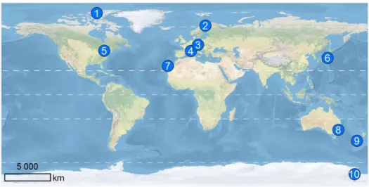
Figure 1. Map of all participating NDACC stations. Detailed coordinates of each station are provided in Table 1.
Table 1. Description of the participating stations.
Latitude Longitude Altitude No. of
Station (◦N) (◦E) (m) daysa Instrument
1 Eureka, EUR (CA) 80.05 −86.42 610 619b Bruker IFS 125HR 2 Kiruna, KIR (SE) 67.84 20.39 420 649 Bruker IFS 120HR Bruker IFS 125HR 3 Zugspitze, ZUG (DE) 47.42 10.98 2954 1114 Bruker IFS 125HR 4 Jungfraujoch, JFJ (CH) 46.55 7.98 3580 1119 Bruker IFS 120HR
5 Toronto, TOR (CA) 43.66 −79.4 174 964 ABB Bomem DA8
6 Tsukuba, TSU (JP) 36.05 140.12 31 640 Bruker IFS 120HR Bruker IFS 125HR 7 Izaña, IZA (ES) 28.29 −16.48 2370 990 Bruker IFS 120M
Bruker IFS 125HR 8 Wollongong, WOL (AU) −34.41 150.88 31 1612 Bomem DA8
Bruker IFS 125HR 9 Lauder, LAU (NZ) −45.04 169.68 370 1017 Bruker IFS 120HR 10 Arrival heights, AHT (NZ) −77.83 166.65 200 341c Bruker IFS 120M aNumber of days with CH
4measurements available over the 2005–2014 time period.bMeasurements started in 2006 and no
measurements between late October and late February due to polar nights.cNo measurements between May and August due to polar
nights.
2.1 Observation sites
Ground-based NDACC FTIR measurements of methane ob-tained at 10 globally distributed observation sites are pre-sented in this study. These sites, displayed in Fig. 1 and whose location is detailed in Table 1 are located from north to south in Eureka (Arctic, Canada), Kiruna (Sweden), Zugspitze (Germany), Jungfraujoch (Switzerland), Toronto (Canada), Tsukuba (Japan), Izaña (Canary Islands, Spain), Wollongong (Australia), Lauder (New Zealand), and Arrival Heights (Antarctica). Most of the FTIR data are available from the NDACC database (http://www.ndsc.ncep.noaa.gov/ data/).
The Eureka (EUR, Fogal et al., 2013) station is located in the Canadian High Arctic, at 610 m a.s.l. on Ellesmere Island
in the northern Canadian Archipelago. The station is located along the Slidre Fjord and is surrounded by complex topogra-phy (Cox et al., 2012). This topogratopogra-phy, along with its prox-imity to the Greenland Ice Sheet and atmospheric conditions, make this station ideal for infrared solar measurements in the Arctic as it is frequently under the influence of cold and dry air from the central Arctic and the Greenland Ice Sheet (Cox et al., 2012). Routine solar infrared measurements are taken from late February to late October; no lunar measurements are taken during polar nights (Batchelor et al., 2009).
The Kiruna (KIR) site is located in the boreal forest re-gion of northern Sweden. The spectrometer is operated in the building of the IRF (Institute för Rymdfysik/Swedish Institute of Space Physics), at an altitude of 420 m, about 10 km away from the centre of Kiruna. The local
popula-tion and traffic density is low, so the FTIR site is not sig-nificantly affected by local anthropogenic emissions. The lo-cation just inside the polar circle is especially suited for the study of the Arctic polar stratosphere, because the break in solar absorption observations is still rather short, while the stratospheric polar vortex frequently covers Kiruna in early spring. The solar absorption spectra were obtained with a Bruker IFS-120HR since 1996. In 2007, an electronic up-grade to a Bruker IFS-125HR was implemented. Routine so-lar infrared measurements are taken between mid-January and mid-November. No lunar measurements are taken dur-ing polar nights.
The Zugspitze (ZUG, Sussmann and Schäfer, 1997) sta-tion is located on the southern slope of the Zugspitze mountain, the highest mountain in the German Alps (2964 m a.s.l.), at the Austrian border near the town of Garmisch-Partenkirchen (720 m a.s.l.). Its high altitude offers an excellent location for long-term trace gas measurements under unperturbed background atmospheric conditions and it exhibits a very low level of integrated water vapour.
The Jungfraujoch (JFJ, Zander et al., 2008) station is lo-cated in the Swiss Alps at an altitude of 3580 m on the saddle between the Jungfrau (4158 m a.s.l.) and the Mönch (4107 m a.s.l.) summits. This station offers unique conditions for infrared solar observations because of weak local pollu-tion (no major industries within 20 km) and very high dry-ness due to the high altitude and the presence of the Aletsch Glacier in its immediate vicinity. The Jungfraujoch station allows for the investigation of the atmospheric background conditions over central Europe and the mixing of air masses between the planetary boundary layer and the free tropo-sphere (Reimann, 2004).
The Toronto (TOR) station is located in the core of the city of Toronto, Ontario, Canada at 174 m a.s.l. where regular so-lar measurements began in 2002. In contrast to most NDACC stations, the Toronto station is highly affected by the densely populated areas of the city of Toronto itself (the centre of Canada’s largest population) and the cities and industrial cen-tres of the north-eastern United States, enabling measure-ments of tropospheric pollutants (Whaley et al., 2015). In ad-dition, the station’s location makes it well suited for measure-ments of midlatitude stratospheric ozone, related species, and greenhouse gases (Wiacek et al., 2007).
The Tsukuba (TSU) station is located in a suburban area (around 50 km from Tokyo) in a large plain with many rice paddies, at an altitude of 31 m. The station occasionally cap-tures local pollution and is affected by high humidity dur-ing the summer season. The Tsukuba solar absorption spec-tra were obtained with a Bruker IFS-120HR from May 2001 to March 2010 and replaced by a Bruker IFS-125HR in April 2010.
The Izaña observatory (IZA, http://www.izana.org) is lo-cated on the top of a mountain plateau in the Teide National Park on the Island of Tenerife. It is usually located above a strong subtropical temperature inversion layer (generally
well established between 500 and 1500 m a.s.l.) and clean-air and clear-sky conditions prevail year-round. Consequently it offers excellent conditions for the remote sensing of trace gases and aerosols under free tropospheric conditions and for atmospheric observations. Due to its geographic location, it is particularly valuable for the investigation of dust port from Africa to the North Atlantic, and large-scale trans-port from the tropics to higher latitudes. In addition, during the daytime the strong insolation generates a slight upslope flow of air originating from below the inversion layer (from a woodland that surrounds the station at a lower altitude; Sepúlveda et al., 2012). The solar absorption spectra were obtained with a Bruker IFS 120M over 1999–2004, then with a Bruker IFS 125HR (Sepúlveda et al., 2012).
Wollongong (WOL, Griffith et al., 1998) is a coastal city about 80 km south of the metropolis of Sydney. Its ur-ban location, in proximity to Sydney and local coal min-ing operations means that enhanced levels of CH4are
mea-sured from time to time. Climatologically the winds are weak (< 4 m s−1); during the Southern Hemisphere winter the site largely samples continental air masses from the west, with summer afternoon sea breezes from the east–north-east (Fraser et al., 2011). The solar absorption spectra were ob-tained with a Bomem DA8 from 1995 to 2007 (Griffith et al., 1998) and with a Bruker IFS 125/HR from 2007 onwards.
The Lauder (LAU) atmospheric research station is located in the Manuherikia valley, Central Otago, New Zealand. The site experiences a continental climate of hot dry summers and cool winters with a predominating westerly wind. The site is sparsely populated and remote from any major industries with non-intense agricultural and horticulture as the mainstay of economic activity.
The Arrival Heights (AHT) atmospheric laboratory is lo-cated 3 km north of McMurdo and Scott Base stations on Hut Point Peninsula, the southern volcanic peninsula of Ross Is-land. With minimal exposure to local anthropogenic pollu-tion and sources, methane measurements conducted at Ar-rival Heights are representative of a well-mixed boundary layer and free troposphere. Located at 78◦S, Arrival Heights is periodically underneath the polar vortex depending on the season, polar vortex shape, and angular rotation velocity. Cli-matological surface meteorological conditions experienced at Arrival Heights are similar to those at Scott Base (Turner et al., 2004). Routine solar infrared measurements are carried out during the austral spring and summer seasons (late Au-gust to mid-April) no measurements are taken during polar nights.
2.2 FTIR observations of methane 2.2.1 Retrieval strategies
A retrieval strategy for the inversion of atmospheric methane time series from ground-based FTIR observations has been carefully developed and optimized for each station. However,
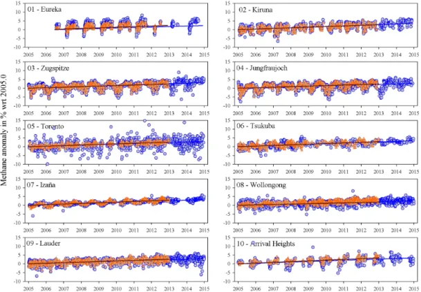
Figure 2. Daily mean methane anomaly with respect to 2005.0 or 2006.0 (in %) for 10 NDACC stations between 2005 and 2014. The blue line is the linear component of the bootstrap fit (see Sect. 3).
it is worth mentioning that given the remaining inconsisten-cies affecting the methane spectroscopic parameters, even in the latest editions of HITRAN (Rothman et al., 2013 and ref-erences therein), the harmonization of retrieval strategies for methane for the whole infrared working group of NDACC is still ongoing. To this day, FTIR measurements are analysed as recommended either by Rinsland et al. (2006), Sussmann et al. (2011), or Sepúlveda et al. (2012). Table A1 presents the retrieval parameters used for each station. The retrieval codes PROFFIT (Hase, 2000) and SFIT-2/SFIT-4 (Rinsland et al., 1998) have been shown to provide consistent results for tropospheric and stratospheric species (Duchatelet et al., 2010; Hase et al., 2004). The time series produced using the strategies described in Table A1 are illustrated in Fig. 2. In order to better illustrate the observed increase of methane total columns, the various panels show daily mean methane time series expressed as anomalies with respect to a reference column in 2005.0 (2006.0 for the Eureka station), according to the following equation:
Anomaly = C − C05 (C + C05) ×1/2
×100, (1)
where C is the methane total column and C05 the methane
total column at the time 2005.0 derived from the linear com-ponent of a Fourier series (Gardiner et al., 2008) fitted to the
time series. The reference columns are given for each station in Table 2. It should be mentioned that the Toronto methane columns from 2008 to early 2009 present a systematic error due to an unknown instrument artefact. The data set was cor-rected by adding a constant offset to the data over that period. To do this, a linear regression was first fit to the full data set (20 June 2002 to 13 December 2014), excluding the biased data, and then another was fit to the biased data only (1 Jan-uary 2008 to 19 March 2009) using the same fixed slope. The difference between the two intercepts gives a constant offset of molecules cm−2, which was added to the biased data.
In order to investigate the possible impact of the choice of the microwindows and spectroscopy on the retrieved methane, each strategy has been tested over a set of spectra recorded at the Jungfraujoch station (3068 spectra recorded between 1 January 2005 and 31 December 2012). Mean frac-tional differences between the strategies described in Table 2 have been computed to quantify a potential absolute bias in terms of total columns and changes over the 2005–2012 time period with the inversion strategy optimized for the Jungfrau-joch observations set as a reference. Mean fractional differ-ences are defined as the difference between two data sets di-vided by their arithmetic average and expressed in percent (see Eq. 2 in Strong et al., 2008). This results in an aver-aged bias between total columns of 0.9 ± 0.5 % but no bias
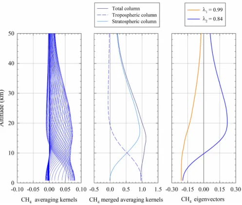
Figure 3. Typical NDACC methane retrieval. From left to right. First panel: typical individual (blue curves) CH4mixing ratio averaging kernels. Second panel: merged (shades of blue curves) CH4mixing ratio averaging kernels. For merged-layer kernels, corresponding atmo-spheric column are specified in the legend box. Third panel: corresponding two first eigenvectors. Associated eigenvalues are given in the legend.
between their respective trends since 2005 is observed (refer-ence values associated with the JFJ strategy in Table A1 are a mean total column of 2.4121±0.0055×10¹⁹molecules cm−2 and a mean annual change of 0.22 ± 0.04 % year−1with re-spect to 2005.0).
2.2.2 Degrees of freedom and vertical sensitivity range Due to the previously mentioned unresolved discrepancies associated with methane spectroscopic parameters, it has been established within the NDACC Infrared Working Group that the regularization strength of the methane retrieval strat-egy should be optimized so that the degrees of freedom for signal (DOFS) is limited to a value of approximately 2 (Suss-mann et al., 2011). As a consequence, the typical informa-tion content of NDACC methane retrievals will allow us to retrieve tropospheric and stratospheric columns, as dis-played in Fig. 3. Indeed, the first eigenvector (in green) and its associated eigenvalue (typically close to 1) show that the corresponding information mainly comes from the retrieval (> 99 %), allowing us to retrieve a partial column ranging from the surface up to 30 km. In addition, the second eigen-vector allows for a finer vertical resolution with two supple-mentary partial columns typically around 1 % of a priori de-pendence: (i) a tropospheric column (typically from the sur-face to the vicinity of the mean tropopause height of the
sta-tion) along with (ii) a stratospheric column (from around the mean tropopause height to 30 km). In terms of error budget, extensive error analysis has been performed by Sepúlveda et al. (2014) and Sussmann et al. (2011). It has been determined that spectroscopic parameters almost exclusively determine the systematic error and amount to ∼ 2.5 % while statistical errors, dominated by baseline uncertainties and measurement noise, sum up to ∼ 1 % (Sepúlveda et al., 2014).
As illustrated in Fig. 3, the information content of our re-trievals sets the upper and lower limits of our tropospheric and stratospheric columns respectively at the vicinity of the mean tropopause height of the station. Therefore, the typical vertical sensitivity range of our retrieval restricts our defini-tion of a purely tropospheric component. Indeed, our tropo-spheric column as previously defined may potentially include a stratospheric contribution due to tropopause altitude varia-tion, hence preventing the sampling of the free tropospheric column in some cases (Sepúlveda et al., 2014).
3 Methane changes since 2005
We characterize the global increase of methane total col-umn from 10 NDACC stations since 2005 and over 10 years’ worth of observations, with a mean annual growth ranging from 0.26 ± 0.02 (Wollongong, 2σ level of uncertainty) to
Table 2. Absolute (in molecules cm−2year−1) and relative (in % year−1) annual change of methane total columns and its associated 2σ -uncertainties from FTIR observations and the GEOS-Chem methane simulation with respect to 2005.0 and to the reference column given in molecules cm−2in the fifth and last columns of this table respectively. The systematic bias between FTIR and GEOS-Chem for 2005–2012 and its associated 2σ -uncertainties are given in the sixth column. A positive bias can be translated into an overestimation of the GEOS-Chem simulation.
FTIR GEOS-Chem
FTIR trend FTIR trend Reference GEOS-Chem trend Reference
(2005–2014) (2005–2012) Column Bias (2005–2012) Column
Unit ×1016molec % yr−1 ×10¹⁶molec % yr−1 ×10¹⁹ % ×1016molec % yr−1 ×10¹⁹
cm−2yr−1 cm−2yr−1 molec cm−2 cm−2yr−1 molec cm−2 EUR 9.54 ± 1.79 0.28 ± 0.05 10.81 ± 3.47 0.32 ± 0.10 3.41∗ 0.9 ± 2.9 12.35 ± 2.06 0.36 ± 0.06 3.46 KIR 13.26 ± 1.46 0.37 ± 0.04 11.7 ± 2.04 0.33 ± 0.06 3.54 −1.0 ± 1.5 12.04 ± 1.66 0.34 ± 0.05 3.53 ZUG 8.33 ± 0.80 0.32 ± 0.03 7.99 ± 1.09 0.31 ± 0.04 2.58 −0.7 ± 1.2 8.09 ± 0.93 0.32 ± 0.04 2.56 JFJ 6.41 ± 0.81 0.27 ± 0.03 5.39 ± 1.04 0.22 ± 0.04 2.40 −0.8 ± 1.5 7.31 ± 0.78 0.31 ± 0.03 2.38 TOR 10.99 ± 3.03 0.29 ± 0.08 12.85 ± 3.76 0.34 ± 0.10 3.71 0.4 ± 5.9 12.45 ± 1.01 0.33 ± 0.03 3.75 TSU 12.99 ± 1.13 0.34 ± 0.03 13.90 ± 1.58 0.36 ± 0.04 3.82 −3.2 ± 3.1 13.36 ± 1.17 0.36 ± 0.03 3.69 IZA 9.56 ± 0.35 0.33 ± 0.01 8.96 ± 0.48 0.31 ± 0.02 2.87 −0.9 ± 1.3 10.34 ± 0.34 0.36 ± 0.01 2.83 WOL 9.62 ± 0.80 0.26 ± 0.02 8.33 ± 1.18 0.23 ± 0.03 3.69 0.6 ± 1.9 13.63 ± 0.74 0.37 ± 0.02 3.69 LAU 9.87 ± 0.95 0.29 ± 0.03 9.81 ± 1.34 0.29 ± 0.04 3.41 2.3 ± 1.7 11.46 ± 1.15 0.33 ± 0.03 3.48 AHT 10.53 ± 2.39 0.32 ± 0.07 9.70 ± 3.48 0.29 ± 0.11 3.28 4.8 ± 3.5 14.53 ± 2.02 0.43 ± 0.06 3.41 Mean 10.11 ± 2.03 0.31 ± 0.03 9.94 ± 2.50 0.30 ± 0.04 – 11.56 ± 2.35 0.35 ± 0.03 –
∗Reference column for Eureka is for 2006.0 since no measurements are available before then. The bottom line of the table shows the average of the 10 mean annual trends.
0.39 ± 0.09 % year−1(Toronto). Observational methane time series anomalies and their changes (along with their associ-ated uncertainties) since 2005.0, illustrassoci-ated in green in Fig. 4 and detailed in Table 2, have been analysed for all 10 sites using the statistical bootstrap resampling tool. They account for a linear component and a Fourier series, taking into ac-count the intra-annual variability of the data set (Gardiner et al., 2008). As in Mahieu et al. (2014), the order of the Fourier series is adapted to each data set depending on its sampling, i.e. limiting the order for the polar sites for which only a partial representation of the seasonality is available. Anoma-lies of methane total column time series, illustrated in Figs. 2 and 5, have been computed using the methane total column computed by the linear component of the statistical bootstrap tool on 1 January 2005, as a reference. Table 2 shows trends of methane total column computed from FTIR observations over the 2005–2014 and 2005–2012 time periods as well as from a tagged GEOS-Chem simulation between 2005 and 2012. The latter is further discussed in Sect. 3.1.2.
On a regional scale, we compared our results with an-nual changes of methane as computed over the 2005–2014 time period from surface GC-MD observations (Gas Chro-matography – MultiDetector) carried out in the framework of the AGAGE programme (Advanced Global Atmospheric Gases Experiment, Prinn et al., 2000) and from in situ sur-face measurements taken in the framework of the NOAA (National Oceanic and Atmospheric Administration) ESRL (Earth System Research Laboratory) carbon cycle air sam-pling network (Dlugokencky et al., 2015). Five representa-tive observation sites have been considered: Alert (Nunavut, Canada, 82.45◦N, −62.51◦E, 200.00 m a.s.l., Dlugokencky
et al., 2015), Mace Head (Ireland, 53.33◦N, −9.90◦E,
Figure 4. Methane total column mean annual change in % year−1 with respect to 2005.0 (2006.0 for Eureka), for the FTIR time se-ries between 2005 and 2014 (in blue), the NDACC FTIR time sese-ries between 2005 and 2012 (in dark blue), and the GEOS-Chem simu-lation between 2005 and 2012 (in orange). Grey error bars represent 2σ uncertainty.
5.00 m a.s.l., Prinn et al., 2000), Izaña (28.29◦N, 16.48◦W,
2372.90 m a.s.l., Dlugokencky et al., 2015), Cape Grim (Australia, 40.68◦S, 144.69◦E, 94.00 m a.s.l., Prinn et al., 2000), and Halley (United Kingdom, 75.61◦S, 26.21◦W, 30.00 m a.s.l., Dlugokencky et al., 2015).
Firstly, in situ measurements collected at Alert, representa-tive of the northern polar region, show an increase of methane of 0.29 ± 0.02 % year−1 (or 5.40 ± 0.41 ppb year−1) since 2006, which is in agreement with our FTIR observations at Eureka with a mean annual change of 0.28 ± 0.05 % year−1. For the northern midlatitudes, we find an agreement between changes of methane as computed from surface measurements at Mace Head with an increase of 0.30 ± 0.02 % year−1 (or 5.58 ± 0.32 ppb year−1) and from our FTIR observa-tions. Indeed, we observe consistent increases of methane of 0.32 ± 0.03, 0.27 ± 0.03, and 0.29 ± 0.08 % year−1since 2005 at Zugspitze, Jungfraujoch, and Toronto. Comparisons between changes of methane from FTIR and in situ sur-face measurements have also been taken for the Izaña sta-tion and show a close to statistical agreement with a mean annual increase of 0.33 ± 0.01 and 0.28 ± 0.02 % year−1 respectively. In the Southern Hemisphere, AGAGE GC-MD measurements of methane at Cape Grim, repre-sentative of the midlatitudes, shows a mean annual in-crease of 0.31 ± 0.01 % year−1 (or 5.40 ± 0.16 ppb year−1) which is in agreement with FTIR changes at Lauder of 0.29 ± 0.03 % year−1. However, we should note the slightly larger mean annual changes of methane of Cape Grim in situ observations with respect to Wollongong FTIR measure-ments. Indeed, it needs to be mentioned that FTIR mea-surements before the instrument change in 2007 (Bomem DA8 vs. Bruker IFS 125HR; see Table 1) show nois-ier results. These noisnois-ier observations at the beginning of the time period under investigation may affect the rel-atively small annual changes of methane overall. As a result, the 2005–2007 time series shows no changes of methane while the 2007–2014 time period shows a mean annual change of 0.32 ± 0.03 % year−1 (or 11.94 ± 1.03 × 10¹⁶molecules cm−2year−1) with respect to 2007.0, which is in agreement with both Lauder FTIR and Cape Grim GC-MD methane changes since 2005. Finally, we computed a mean annual change of methane of 0.32 ± 0.01 % year−1 (or 5.45 ± 0.14 ppb year−1) from in situ surface measure-ments taken at Halley, which is in good agreement with the mean annual change of methane computed from FTIR Ar-rival Heights retrievals that amounts to 0.32 ± 0.07 % year−1. In summary, we observe from NDACC FTIR measure-ments a global average annual change of methane of 0.31 ± 0.03 % year−1 (averaged over 10 stations, 2σ level of uncertainty) which is in agreement with a mean annual change of 0.31 ± 0.01 % year−1(or 5.51 ± 0.17 ppb year−1), as computed from the monthly global means of baseline data derived from AGAGE measurements (Prinn et al., 2000).
In addition, analyses of tropospheric and stratospheric partial columns changes show tropospheric mean annual changes of methane that are statistically in agreement (at the 2σ level) with changes of total column over the 2005– 2014 time period. Mean annual changes from the Atmo-spheric Chemistry Experiment Fourier transform spectrom-eter methane research product (ACE-FTS, Bernath et al.,
2005) have also been examined. For consistent comparison, ACE-FTS stratospheric columns of methane have been de-fined in the same way as the stratospheric FTIR product, i.e. from the average tropopause height of the station to 30 km. Changes of stratospheric methane according to ACE-FTS retrievals are statistically in agreement with our NDACC FTIR changes of stratospheric columns and show small to non-significant changes of methane in the stratosphere. In-deed, changes of stratospheric methane according to the ACE-FTS methane research product (Buzan et al., 2016) are not significant and amount to −0.12 ± 0.13 % year−1for the northern high latitudes, 0.10 ± 0.30 for northern midlat-itudes, 0.08 ± 0.24 for the tropical region, −0.10 ± 0.31 for the southern midlatitudes, and −0.04 ± 0.14 % year−1for the southern high latitudes.
3.1 GEOS-Chem-tagged simulation
GEOS-Chem (version 9-02: http://acmg.seas.harvard.edu/ geos/doc/archive/man.v9-02/index.html, Turner et al., 2015) is a global 3-D chemistry transport model (CTM) capa-ble of simulating global trace gas and aerosol distributions. GEOS-Chem is driven here by assimilated meteorological fields from the Goddard Earth Observing System version 5 (GEOS-5) of the NASA Global Modeling Assimilation Office (GMAO). The GEOS-5 meteorological data have a temporal frequency of 6 h (3 h for mixing depths and sur-face properties) and are at a native horizontal resolution of 0.5◦×0.667◦ with 72 hybrid pressure-σ levels describing the atmosphere from the surface up to 0.01 hPa. In the frame-work of this study, the GEOS-5 fields are degraded for model input to a 2◦×2.5◦horizontal resolution and 47 vertical levels
by collapsing levels above ∼ 80 hPa. GEOS-Chem has been extensively evaluated in the past (van Donkelaar et al., 2012; Park et al., 2006, 2004; Zhang et al., 2011, 2012). These stud-ies show a good simulation of global transport with no appar-ent biases.
Emissions for the GEOS-Chem simulations are from the EDGAR v4.2 anthropogenic methane inventory (European Commission, 2011), the wetland model from Kaplan (2002) as implemented by Pickett-Heaps et al. (2011), the GFED3 biomass burning inventory (van der Werf et al., 2010), a ter-mite inventory and soil absorption from Fung et al. (1991), and a biofuel inventory from Yevich and Logan (2003). Wetland emissions vary with local temperature, inundation, and snow cover. Open fire emissions are specified with 8 h temporal resolution. Other emissions are assumed seasonal. Methane loss is mainly by reaction with the OH radical. We use a 3-D archive of monthly average OH concentrations from Park et al. (2004). The resulting atmospheric lifetime of methane is 8.9 years, consistent with the observational con-straint of 9.1 ± 0.9 years (Prather et al., 2012).
The GEOS-Chem model output presented here covers the period January 2005–December 2012, for which the GEOS-5 meteorological fields are available. For this simulation, we
use the best emission inventories available as implemented in version 9-02 of the model and rely on the spatial and tem-poral distributions of emissions. This tagged simulation in-cludes 11 tracers: 1 tracer for the soil absorption sink (sa) and 10 tracers for sources: gas and oil (ga), coal (co), live-stock (li), waste management (wa), biofuels (bf), rice culti-vation (ri), biomass burning (bb), wetlands (wl), other natural emissions (on) and other anthropogenic (oa) emissions. We have used a 1-year run for spin-up from January to Decem-ber 2004, restarted 70 times for initialization of the tracer concentrations. The model outputs consist of methane mix-ing ratio profiles saved at a 3 h time frequency and at the clos-est pixel to each NDACC station. To account for the vertical resolution and sensitivity of the FTIR retrievals, the individ-ual concentration profiles simulated by GEOS-Chem are in-terpolated onto the FTIR vertical grid (see next section for description of regridding).
3.1.1 Data regridding and processing
In order to perform a proper comparison between the GEOS-Chem outputs and our NDACC FTIR observations, we ac-counted for their respective spatial domains and used a con-servative regridding scheme so that the total mass of the tracer is preserved (both locally and globally over the en-tire vertical profile). This was achieved using an algorithm similar to the one described in Sect. 3.1 of Langerock et al. (2015). To this end, time-dependent elevation coordi-nates are first calculated for the model outputs using grid-box height data and topography data are regridded onto the GEOS-Chem horizontal grid before conservative regridding. The model outputs (source grid) are then regridded onto an observation-compliant destination grid through our conser-vative regridding scheme that includes a nearest-neighbour interpolation and a vertical regridding. The vertical destina-tion grid corresponds to the retrieval grid adopted for each station. Regridded fields (tracer mixing-ratio) may have un-defined values for cells of the destination grid that do not overlap with the model source grid. For grid cells that par-tially overlap the model grid, we apply a “mask tolerance”, i.e., a relative overlapping volume threshold below which the value of the grid cell will be set as undefined. This may intro-duce conservation errors, but since partially overlapping cells are likely to occur only at the top level of the model vertical grid, these errors can be neglected for species that usually have a low mixing ratio at that level, such as methane.
To account for the vertical resolution and sensitivity of the FTIR retrievals, the individual concentration profiles simu-lated by GEOS-Chem are averaged into daily profiles (in-cluding day and night simulation) and smoothed according to:
xsmooth=xa+A (xm−xa) , (2)
where A is the FTIR averaging kernels, xmis the daily mean
profile as simulated by the GEOS-Chem model regridded to
the observation retrieval grid and xathe FTIR a priori used in
the retrieval according to the formalism of Rodgers (1990). Averaging kernels are seasonal averages combining individ-ual matrices from FTIR retrievals. Concerning the methane tracers, we constructed vertical a priori profiles for each of them by scaling the methane a priori employed for each sta-tion in order to smooth them as well. To this end, we deter-mined for the 10 sites the contribution of each tracer to the total methane on the basis of the mean budget simulated by the model over the 2005–2012 time period.
3.1.2 GEOS-Chem simulation vs NDACC FTIR observations
As we previously pointed out, since the information content of the FTIR retrievals prevents a pure tropospheric compo-nent from being retrieved, we will focus on comparisons between FTIR and GEOS-Chem total columns. Due to the availability of the GEOS-5 meteorological fields and to en-sure consistency, we limited our comparison of methane changes between FTIR observations and the GEOS-Chem simulation over the 2005–2012 time period. It is, however, worth mentioning that methane changes as observed by our FTIR observations are in agreement for all 10 stations (see Fig. 4 and Table 2) between both time periods, i.e. 2005– 2012 and 2005–2014.
Firstly, comparisons between FTIR observations and the smoothed GEOS-Chem simulation over the 2005–2012 time period have been performed for each NDACC station on days when observations are available. Both time series are illus-trated in Fig. 5 as anomalies with respect to 2005.0 (see cor-responding reference columns in Table 3). We report a good agreement between FTIR and GEOS-Chem methane with no systematic bias (see definition of mean fractional differences given in Sect. 2.2.1 and Eq. 2 in Strong et al., 2008), ex-cept for the Tsukuba, Lauder and Arrival Heights stations where GEOS-Chem shows a systematic bias of −3.2 ± 3.1, 2.3 ± 1.7, and 4.8 ± 3.5 % (2σ level of uncertainty), with their respective FTIR observations. Since we defined the methane anomaly at 0 % in 2005.0 (or 2006.0 for Eureka) for both our observations and the GEOS-Chem simulation, we consequently corrected this observed bias in Fig. 5. On the other hand, we observe a slight phase offset between FTIR and GEOS-Chem seasonal cycles for Izaña and Tsukuba. Indeed, GEOS-Chem simulates the maximum methane col-umn 85 days ahead of FTIR measurements for Izaña while it shows a delay of 92 days with respect to the Tsukuba FTIR time series. It should, however, be pointed out that the sea-sonal cycle’s amplitude is well reproduced by GEOS-Chem with a peak-to-peak amplitude of 5.0 ± 0.9 % for Tsukuba and of 3.6 ± 0.5 % for Izaña while the methane seasonal cy-cle from FTIR measurements shows a peak-to-peak ampli-tude of 5.9 ± 1.7 and 4.3 ± 1.8 % respectively.
Regarding the increase of methane, the simulation by GEOS-Chem indicates a mean annual increase ranging from
Figure 5. Daily mean CH4total column anomalies with respect to 2005.0 (in %) for 10 NDACC stations between 2005 and 2014 for NDACC FTIR observations (in blue) and between 2005 and 2012 for the smoothed GEOS-Chem simulation (in orange) along with their respective linear component of the bootstrap fit in blue and brown.
0.31 ± 0.03 to 0.43 ± 0.06 % year−1 and a globally aver-aged annual change of 0.35 ± 0.03 % year−1with respect to 2005.0 (averaged over 10 stations, 2σ level of uncertainty). Mean annual changes of total columns of methane between 2005 and 2012 for both FTIR measurements and the GEOS-Chem simulation are illustrated in Fig. 4 in blue and orange respectively. In terms of the methane increase, the model is in good agreement (within error bars) with the observations ex-cept for Jungfraujoch, Izaña, and Wollongong where GEOS-Chem shows an overestimation of the methane increase.
We first discuss the possible causes of the slight trend discrepancy between FTIR observations at Jungfraujoch and Zugspitze as well as with GEOS-Chem for both stations. In-deed, despite their proximity (∼ 250 km apart) and their re-spective altitude of 3580 and 2954 m, both Alpine sites show distinct influences from local thermal-induced vertical trans-port. At mountain-type sites, subsidence is predominant for anticyclonic weather conditions, resulting in adiabatic warm-ing and cloud dissipation. The clear-sky and strong radia-tion condiradia-tions lead to the convective growth of the atmo-spheric boundary layer (ABL) and induce thermal injections of ABL air to the high-altitude observation sites (Collaud Coen et al., 2011; Henne et al., 2005; Nyeki et al., 2000). In addition, mountain venting induced by higher tempera-tures allows ABL air to be transported to the free tropo-sphere, often occurring in summer (between April and
Au-gust; Henne et al., 2005; Kreipl, 2006). While the Jungfrau-joch site is a remote site, mostly influenced by free tropo-spheric air masses with incursions of ABL air masses dur-ing 50 % of the sprdur-ing and summer (Collaud Coen et al., 2011; Henne et al., 2005, 2010; Okamoto and Tanimoto, 2016; Zellweger et al., 2000, 2003), the Zugspitze site is more often influenced by the ABL (Henne et al., 2010). In summer, when the influence of the ABL is the largest, the observed changes are in very close agreement, with 0.25 ± 0.06 and 0.26 ± 0.09 % year−1 respectively. More-over, it has been established that vertical export of air masses above mountainous terrain is presently poorly represented in global CTMs (Henne et al., 2004). Mean annual changes of GEOS-Chem methane agree with the observations in sum-mer during the influence of the ABL, with 0.33 ± 0.04 and 0.27 ± 0.08 % year−1for Jungfraujoch and Zugspitze respec-tively. In contrast, GEOS-Chem shows mean annual win-ter changes of 0.23 ± 0.11 and 0.19 ± 0.09 % year−1 which agree with observed changes at Zugspitze but not with changes at Jungfraujoch. Since comparisons between FTIR measurements and GEOS-Chem methane show a disagree-ment on the methane changes during winter at Jungfraujoch, this seasonal analysis of changes of methane at mountain-ous observation sites emphasizes the current poorly modelled representation of summer versus winter thermal convection of air masses from the boundary layer to the free troposphere.
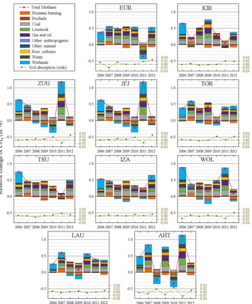
Figure 6. Year-to-year relative changes in CH4total columns due to each emission source (see colour codes) for each station (see codes in Table 1) derived from GEOS-Chem. Brown circles represent the year-to-year relative changes of the methane sink due to soil absorption. Red circles illustrate the cumulative year-to-year methane change.
Regarding Izaña, it is worth mentioning that the FTIR methane total column time series shows a smaller seasonal cycle. Indeed, the combination of no local emission sources in the vicinity of Izaña, good mixing of air masses and a regular solar insolation associated with more constant OH amounts leads to a dampened seasonal cycle (Dlugokencky et al., 1994) at that site. Therefore, small annual changes of methane and smaller uncertainty on the mean annual change computed by the bootstrap method complicates the agree-ment between the FTIR and GEOS-Chem methane changes. However, as mentioned above, it should be pointed out that the amplitude of this smaller seasonal cycle is well repro-duced by the GEOS-Chem simulation.
Regarding Wollongong, as already pointed out, noisier ob-servations at the beginning of the period of interest may
af-fect the relatively small annual changes of methane overall. In addition, one should not forget that sites such as Izaña or Wollongong can be challenging sites for models to reproduce due to the topography and land–sea contrast (Kulawik et al., 2016).
3.1.3 Tagged simulation analysis
The GEOS-Chem-tagged simulation, which provides the contribution of each tracer to the total simulated methane, enables us to quantify and express the contribution of each tracer to the global methane increase. In order to do so, we considered year-to-year relative changes according to the
fol-lowing equation:
Y C (in %) = (µn−µn−1) µtot,n−1
, (3)
where µn is the annual mean of the simulated methane for
the year n. The year-to-year relative changes are computed so that when we assume a relative change of a tracer for the year n, it is expressed with respect to the previous year (n −1) using µtot,n−1 the annual mean of the simulated
cu-mulative methane for the year (n − 1) as a reference. Aver-ages of the individual relative year-to-year changes of total methane are in agreement with the mean annual change com-puted by the bootstrap method within error bars (2σ level uncertainty; Table 2). Therefore, the considered relative year-to-year changes of each tracer and for each site are illustrated in Fig. 6. The first three contributors to the annual methane change over the 2005–2012 time period are displayed for each site in Table B1 (see Appendix B) along with the cumu-lative recumu-lative increase for the whole 2005–2012 time period. On a global scale, we observe from the tracer analysis as simulated by GEOS-Chem that natural emission sources such as emissions from wetlands and biomass burning fluc-tuate interannually, thus are the dominant contributors to the interannual variability in methane surface emissions. This is in agreement with the finding of Bousquet et al. (2011), who report that fluctuations in wetland emissions are the domi-nant contribution to interannual variability in surface emis-sions, explaining 70 % of the global emission anomalies over the past 2 decades, while biomass burning contributes only 15 %. Regarding wetland emissions, the simulation shows a mean net increase of methane in 2006 of +0.30 % (mean value over all sites) attributed to the tracer. In 2007–2008, GEOS-Chem simulates a stabilization of methane in the at-mosphere due to the reduction of wetland emissions. In-deed, we observe either a slightly negative change in wet-land methane of −0.08 ± 0.07 and of −0.08 ± 0.04 % re-spectively in 2008 and 2009 (mean values over all sites) or a minor increase not larger than 0.07 % in Arrival Heights (in 2009), in Tsukuba (in 2008) and in the high-latitude sites (i.e. Eureka and Kiruna in 2008 and 2009). On the other hand, the biomass burning tracer globally shows a net increase of 0.10 ± 0.01 % in 2007 likely due to the major fire season in tropical South America (Bloom et al., 2015) and a net de-crease of −0.09 ± 0.01 % in 2009 and of −0.07 ± 0.01 % in 2012 with respect to the previous year. On the sink side, we find a negative phase between the relative year-to-year changes of the soil absorption tracer and the total methane simulated by GEOS-Chem except for Izaña where it remains positive over the time period studied.
On a local scale, we observe a slow-down of the increase in 2010 at midlatitude sites (i.e. Zugspitze, Jungfraujoch, Toronto) and in 2011 at Tsukuba and at the high-latitude sites of Eureka and Kiruna. Following this stabilization phase, Eu-ropean sites find a substantial increase of more than 1.15 % in 2011 with respect to the previous year which is mainly
due to an anomaly of wetlands emissions (+0.38 %) but also as a result of a relative increase of +0.21 and +0.17 % of emissions from livestock and coal. The Izaña site presents the most regular increase, mainly due to a smaller variabil-ity over the whole time period (seasonal cycle of Izaña pre-viously discussed in Sect. 3.1.2.). In contrast, methane over Arrival Heights shows high variability from one year to an-other, which illustrates how dynamically sensitive the polar air is to transport from lower latitudes (Strahan et al., 2015). Finally, regarding anthropogenic emissions, with positive year-to-year changes during the whole 2005–2012 time pe-riod, the coal and the gas and oil emissions both regu-larly increase over time. According to the GEOS-Chem-tagged simulation, they rank as the most important anthro-pogenic contributors to methane changes for all stations (see Appendix B) and thus substantially contribute to the total methane increase. In fact, the coal and the gas and oil tracers respectively comprise a third (32 %) and almost a fifth (18 %) of the cumulative increase of methane over the 2005–2012 time period while their respective emissions are responsible for only 7.5 and 12.5 % of the methane budget. As a compar-ison, the cumulative increase of methane emitted from wet-lands amounts to 16 % of the total increase since 2005, while wetland emissions make up 34 % of the methane budget.
4 Discussion and conclusions
The cause of the methane increase since the mid-2000s has often been discussed and still has not been completely re-solved (Aydin et al., 2011; Bloom et al., 2010; Dlugokencky et al., 2009; Hausmann et al., 2016; Kirschke et al., 2013; Nisbet et al., 2014; Rigby et al., 2008; Ringeval et al., 2010; Schaefer et al., 2016; Sussmann et al., 2012). On the sink side, Rigby et al. (2008) identified a decrease of OH rad-icals with a large uncertainty (−4 ± 14 %) from 2006 to 2007 while Montzka et al. (2011) found a small drop of ∼1 % year−1, which might have contributed to the enhanced methane in the atmosphere. On the other hand, Bousquet et al. (2011) reported that the changes in OH remain small (< 1 % over the 2006–2008 time period). Nevertheless, ob-servations of small interannual variations are in agreement with the understanding that perturbations in the atmospheric composition generally buffer the global OH concentrations (Dentener, 2003; Montzka et al., 2011).
The small to non-significant changes of methane in the stratosphere, as reported from the analysis of the ACE-FTS methane research product, confirm that the increase of methane takes place in the troposphere. It is indeed driven by increasing sources emitted from the ground (Bousquet et al., 2011; Nisbet et al., 2014; Rigby et al., 2008), primarily affecting its tropospheric abundance and justifying the need for a source-oriented analysis of this recent increase.
Our analysis of the GEOS-Chem-tagged simulation de-termines that secondary contributors to the global budget
of methane, such as coal mining and gas and oil transport and exploitation, have played a major role in the increase of atmospheric methane observed since 2005. However, while the simulation we used comprises the best emission inven-tories available so far, it has its limitations. Firstly, Schwi-etzke et al. (2014), Bergamaschi et al. (2013) and Bruh-wiler et al. (2014) reported that the EDGAR v4.2 emis-sion inventory overestimates the recent emisemis-sion growth in Asia. Indeed, Turner et al. (2015) reported from a global GOSAT (Greenhouse gases Observing SATellite) inversion that Chinese methane emissions from coal mining are too large by a factor of 2. Other regional discrepancies between the EDGAR v4.2 inventory and the GOSAT inversion such as an increase in wetland emissions in South America and an increase in rice emissions in South-east Asia, have been pointed out by Turner et al. (2015) as well. On the other hand, it has been shown that the current emissions invento-ries, including EDGAR v4.2, underestimate the emissions of methane associated with the gas and oil use and exploitation, as well as livestock emissions (Franco et al., 2015, 2016; Turner et al., 2015, 2016). Furthermore, Lyon et al. (2016) pointed out that emissions from oil and gas well pads may be missing from most bottom-up emission inventories. The problem of the source identification clearly resides in the need for a better characterization of anthropogenic emissions and especially in emissions of methane from the oil and gas and livestock sectors.
Concerning the oil and gas emissions, ethane has shown a sharp increase since 2009 of ∼ 5 % year−1at midlatitudes and of ∼ 3 % year−1 at remote sites (Franco et al., 2016) which is attributed to the recent massive growth of oil and gas exploitation in the North American continent, with the geo-graphical origin of these additional emissions confirmed by Helmig et al. (2016). Since ethane shares an anthropogenic source of methane, i.e. the production, transport and use of natural gas and the leakage associated to it (at 62 %; Logan et al., 1981; Rudolph, 1995), Franco et al. (2016) were able to estimate an increase of oil and gas methane emissions rang-ing from 20 Tg year−1in 2008 to 35 Tg year−1in 2014, using the C2H6/CH4ratio derived from GOSAT measurements as
a proxy, confirming the influence of fossil fuel and gas pro-duction emissions impact on the observed methane increase. Moreover, Hausmann et al. (2016) reported an oil and gas contribution to the renewed methane in Zugspitze of 39 % over the 2007–2014 time period based on a C2H6/CH4
ra-tio derived from an atmospheric two-box model. However, as Kort et al. (2016) and Peischl et al. (2016) pointed out, the variability in the C2H6/CH4ratio associated to oil and gas
production needs to be taken into account in a more rigor-ous manner as the strength of the C2H6/CH4 relationship
strongly depends on the studied region and/or production basin.
In conclusion, we report changes of atmospheric methane between 2005 and 2014 from FTIR measurements taken at 10 ground-based NDACC observation sites for the first time.
From the 10 NDACC methane time series, we computed a mean global annual increase of total column methane of 0.31 ± 0.03 % year−1 (averaged over 10 stations, 2σ level of uncertainty), using 2005.0 as reference, which is consis-tent with methane changes computed from in situ measure-ments. From the GEOS-Chem-tagged simulation, accounting for 11 tracers (10 emission sources and one sink) and cov-ering the 2005–2012 time period, we computed a mean an-nual change of methane of 0.35 ± 0.03 % year−1since 2005, which is globally in good agreement with the FTIR mean an-nual changes. In addition, we presented a detailed analysis of the GEOS-Chem tracer changes on both global and lo-cal slo-cales over the 2005–2012 time period. To this end, we considered relative year-to-year changes in order to quantify the contribution of each tracer to the global methane change since 2005. According to the GEOS-Chem tagged simula-tion, wetland methane contributes mostly to the interannual variability while sources that contribute the most to the ob-served increase of methane since 2005 are mainly anthro-pogenic: coal mining, gas and oil exploitation, and livestock (from largest to smallest contribution). While we showed that GEOS-Chem agrees with our observations and consequently with the in situ measurements, the repartition between the different sources of methane would greatly benefit from an improvement of the global emission inventories. As an exam-ple, Turner et al. (2015) suggested that EDGAR v4.2 under-estimates the US oil and gas and livestock emissions while overestimating methane emissions associated to coal mining. From the emission source shared by both ethane and methane and from various ethane studies, it is clear that further atten-tion has to be given to improved anthropogenic methane in-ventories, such as emission inventories associated with fossil fuel and natural gas production. This is essential in a con-text of the energy transition that includes the development of shale gas exploitation.
Finally, it is worth mentioning that Schaefer et al. (2016) argue with the fact that thermogenic emissions of methane are responsible for the renewed increase of methane during the mid-2000s. Indeed, from methane isotopologue observa-tions and a one-box model deriving global emission strength and isotopic source signature, Schaefer et al. (2016) reports that the recent methane increase is predominantly due to biogenic emission sources such as agriculture and climate-sensitive natural emissions. These results contrast with the context of a booming natural gas production and the resump-tion of coal mining in Asia. However, it is also worth noting that the 13C /12C and D / H ratio of atmospheric methane show distinctive isotope signature depending on the source type (Bergamaschi, 1997; Bergamaschi et al., 1998; Quay et al., 1999; Snover et al., 2000; Whiticar and Schaefer, 2007). In the same way, isotopic fractionation occurs during sink processes with specific ratios depending on the removal path-way (Gierczak et al., 1997; Irion et al., 1996; Saueressig et al., 2001; Snover and Quay, 2000; Tyler et al., 2000). There-fore, the underexploited analysis of the recent methane
in-crease through trend analysis of methane isotopologues, such as13CH4and CH3D, is an innovative way of addressing the
question of the source(s) responsible for the recent methane increase.
5 Data availability
Most of the data used in this publication were obtained as part of the Network for the Detection of Atmospheric Com-position Change (NDACC) and are publicly available (see http://www.ndacc.org). Time series used to produce Fig. 5, as well as GEOS-Chem-tagged simulation time series, can
be found on the University of Liège’s repository (see http: //orbi.ulg.ac.be/handle/2268/207090). In situ surface mea-surements taken in the framework of the NOAA ESRL car-bon cycle air sampling network (Dlugokencky et al., 2015; version: 2015-08-03; date accessed: 9 May 2016) are avail-able at ftp://aftp.cmdl.noaa.gov/data/trace_gases/ch4/flask/ surface/. Surface GC-MD observations carried out in the framework of the AGAGE programme (Prinn et al., 2000; date accessed: 9 May 2016) are available at http://agage.eas. gatech.edu/data_archive/agage/gc-md/.
Appendix A: NDACC FTIR retrieval strategies
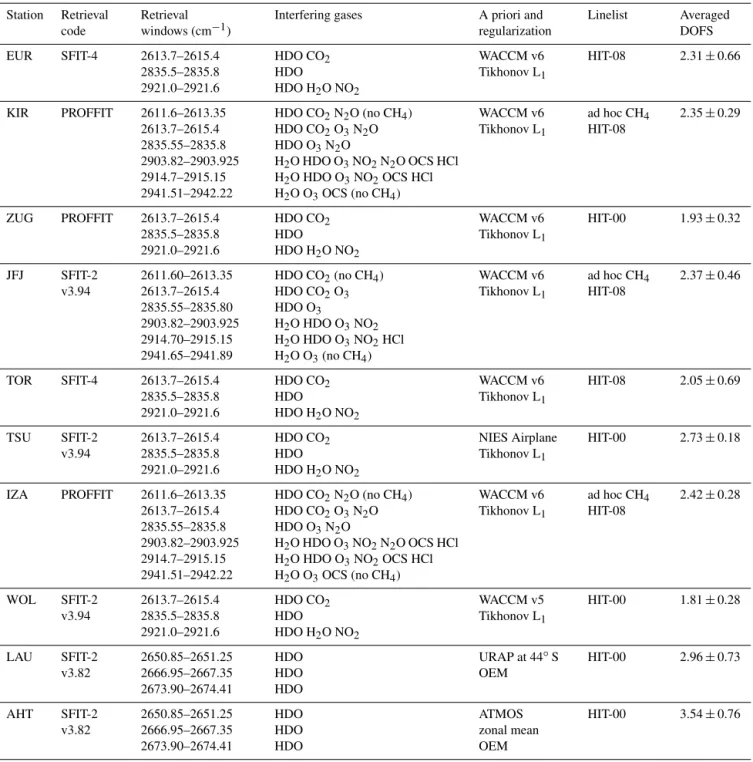
Table A1 summarizes the retrieval parameters for methane for each station. FTIR measurements are analysed as rec-ommended either by Rinsland et al. (2006), Sussmann et al. (2011), or Sepúlveda et al. (2012). The spectral microwin-dows limits for the Eureka, Zugspitze, Toronto and Wol-longong stations are based on Sussmann et al. (2011) and use the Hitran-2000 spectroscopic database including the re-lease of the 2001 update (Rothman et al., 2003) except for Toronto where Hitran 2008 was employed (Rothman et al., 2009). The microwindows used for the Kiruna, Jungfraujoch, Izaña observations are based on Sepulveda et al. (2012). For all interfering species, Hitran 2008 parameters are used. For methane, ad hoc adjustments carried out by KIT, IMK-ASF are used (D. Dubravica, personal communication, Decem-ber 2012; see also Dubravica et al., 2013). Finally, the mi-crowindows used for the Lauder and Arrival Heights obser-vations are based on Rinsland et al. (2006). In order to better appraise the relatively low humidity rates at Jungfraujoch, a prefitting of the two microwindows (2611.60–2613.35 and 2941.65–2941.89) dedicated to water vapour and its isotopo-logue HDO is performed and used as a priori for the actual retrieval.
A priori profiles for target and interfering molecules are based on the Whole Atmosphere Community Climate Model
(version 5 or 6, WACCM, e.g. Chang et al., 2008) clima-tology, except for Tsukuba, Lauder, and Arrival Heights. A priori profiles for Tsukuba retrievals include monthly av-eraged profiles made from aeroplane measurements over Japan by the National Institute of Environmental Studies, Japan (NIES, http://www.nies.go.jp/index-e.html). A priori profiles for Lauder retrieval include annual mean of mea-surements from the Microwave Limb Sounder (MLS, https: //mls.jpl.nasa.gov/) and the Halogen Occultation Experi-ment (HALOE, http://haloe.gats-inc.com/home/index.php) on board the Upper Atmosphere Research Satellite (UARS, http://uars.gsfc.nasa.gov/) at 44◦S in the framework of the UARS Reference Atmosphere Project (URAP, Grooß and Russell, 2005). A priori profiles for Arrival Heights retrievals include the zonal mean of measurements from the Atmo-spheric Trace Molecule Spectroscopy Experiment (ATMOS) Spacelab 3 over the 14–65 km altitude range (Gunson et al., 1996). As mentioned in the Sect. 2.2.2. of this paper, a Tikhonov regularization (Tikhonov, 1963) is used and opti-mized in order to limit the value of the degrees of freedom for signal (DOFS) to a value of approximately 2 (Sussmann et al., 2011) except for Lauder and Arrival Heights which use an optimal estimation method (OEM) based on the formalism of Rodgers (1990). Averaged DOFS value and associated 1σ uncertainty are given in the last column of Table A1.
Table A1. Retrieval parameters for each station.
Station Retrieval code
Retrieval windows (cm−1)
Interfering gases A priori and
regularization Linelist Averaged DOFS EUR SFIT-4 2613.7–2615.4 2835.5–2835.8 2921.0–2921.6 HDO CO2 HDO HDO H2O NO2 WACCM v6 Tikhonov L1 HIT-08 2.31 ± 0.66 KIR PROFFIT 2611.6–2613.35 2613.7–2615.4 2835.55–2835.8 2903.82–2903.925 2914.7–2915.15 2941.51–2942.22 HDO CO2N2O (no CH4) HDO CO2O3N2O HDO O3N2O H2O HDO O3NO2N2O OCS HCl H2O HDO O3NO2OCS HCl H2O O3OCS (no CH4) WACCM v6 Tikhonov L1 ad hoc CH4 HIT-08 2.35 ± 0.29 ZUG PROFFIT 2613.7–2615.4 2835.5–2835.8 2921.0–2921.6 HDO CO2 HDO HDO H2O NO2 WACCM v6 Tikhonov L1 HIT-00 1.93 ± 0.32 JFJ SFIT-2 v3.94 2611.60–2613.35 2613.7–2615.4 2835.55–2835.80 2903.82–2903.925 2914.70–2915.15 2941.65–2941.89 HDO CO2(no CH4) HDO CO2O3 HDO O3 H2O HDO O3NO2 H2O HDO O3NO2HCl H2O O3(no CH4) WACCM v6 Tikhonov L1 ad hoc CH4 HIT-08 2.37 ± 0.46 TOR SFIT-4 2613.7–2615.4 2835.5–2835.8 2921.0–2921.6 HDO CO2 HDO HDO H2O NO2 WACCM v6 Tikhonov L1 HIT-08 2.05 ± 0.69 TSU SFIT-2 v3.94 2613.7–2615.4 2835.5–2835.8 2921.0–2921.6 HDO CO2 HDO HDO H2O NO2 NIES Airplane Tikhonov L1 HIT-00 2.73 ± 0.18 IZA PROFFIT 2611.6–2613.35 2613.7–2615.4 2835.55–2835.8 2903.82–2903.925 2914.7–2915.15 2941.51–2942.22 HDO CO2N2O (no CH4) HDO CO2O3N2O HDO O3N2O H2O HDO O3NO2N2O OCS HCl H2O HDO O3NO2OCS HCl H2O O3OCS (no CH4) WACCM v6 Tikhonov L1 ad hoc CH4 HIT-08 2.42 ± 0.28 WOL SFIT-2 v3.94 2613.7–2615.4 2835.5–2835.8 2921.0–2921.6 HDO CO2 HDO HDO H2O NO2 WACCM v5 Tikhonov L1 HIT-00 1.81 ± 0.28 LAU SFIT-2 v3.82 2650.85–2651.25 2666.95–2667.35 2673.90–2674.41 HDO HDO HDO URAP at 44◦S OEM HIT-00 2.96 ± 0.73 AHT SFIT-2 v3.82 2650.85–2651.25 2666.95–2667.35 2673.90–2674.41 HDO HDO HDO ATMOS zonal mean OEM HIT-00 3.54 ± 0.76
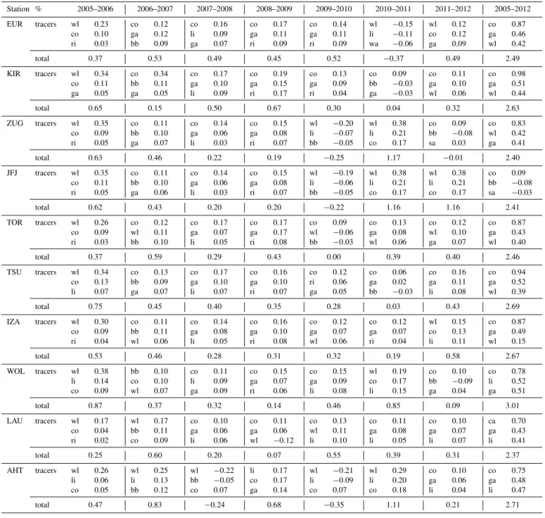
Appendix B: Top three contributors to the methane increase as simulated by GEOS-Chem
Table B1 illustrates the first three contributors to the annual methane change and their year-to-year changes for each site along with the cumulative relative increase for the whole 2005–2012 time period. The GEOS-Chem tracers are coded as follows: biomass burning (bb), biofuels (bf), coal (co), livestock (li), gas and oil (ga), other anthropogenic sources (oa), other natural sources (on), rice cultivation (ri), waste management (wa), wetlands (wl).
Table B1. Top three simulated tracers contributing the most to the methane changes, per year, and per site, in %.
Station % 2005–2006 2006–2007 2007–2008 2008–2009 2009–2010 2010–2011 2011–2012 2005–2012 EUR tracers wl co ri 0.23 0.10 0.03 co ga bb 0.12 0.12 0.09 co li ga 0.16 0.09 0.07 co ga ri 0.17 0.11 0.09 co ga ri 0.14 0.11 0.09 wl li wa −0.15 −0.11 −0.06 wl co ga 0.12 0.12 0.09 co ga wl 0.87 0.46 0.42 total 0.37 0.53 0.49 0.45 0.52 −0.37 0.49 2.49 KIR tracers wl co ga 0.34 0.11 0.05 co bb ga 0.34 0.11 0.05 co ga li 0.17 0.10 0.09 co ga ri 0.19 0.15 0.17 co ga ri 0.13 0.09 0.04 co bb ga 0.09 −0.03 −0.03 co ga wl 0.11 0.10 0.06 co ga wl 0.98 0.51 0.44 total 0.65 0.15 0.50 0.67 0.30 0.04 0.32 2.63 ZUG tracers wl co ri 0.35 0.09 0.05 co bb ga 0.11 0.10 0.07 co ga li 0.14 0.06 0.03 co ga ri 0.15 0.08 0.07 wl li bb −0.20 −0.07 −0.05 wl li co 0.38 0.21 0.17 co bb sa 0.09 −0.08 0.03 co wl ga 0.83 0.42 0.41 total 0.63 0.46 0.22 0.19 −0.25 1.17 −0.01 2.40 JFJ tracers wl co ri 0.35 0.11 0.05 co bb ga 0.11 0.10 0.06 co ga li 0.14 0.06 0.03 co ga ri 0.15 0.08 0.07 wl li bb −0.19 −0.06 −0.05 wl li co 0.38 0.21 0.17 wl li co 0.38 0.21 0.17 co bb sa 0.09 −0.08 −0.03 total 0.62 0.43 0.20 0.20 −0.22 1.16 1.16 2.41 TOR tracers wl co ri 0.26 0.09 0.03 co wl bb 0.12 0.11 0.10 co ga li 0.17 0.07 0.05 co ga ri 0.17 0.17 0.08 co wl bb 0.09 −0.06 −0.03 co ga wl 0.13 0.08 0.06 co wl ga 0.12 0.10 0.07 co ga wl 0.87 0.43 0.40 total 0.37 0.59 0.29 0.43 0.00 0.39 0.40 2.46 TSU tracers wl co li 0.34 0.13 0.07 co bb ga 0.13 0.09 0.07 co ga li 0.17 0.10 0.07 co ga ri 0.16 0.10 0.07 co ri ga 0.12 0.06 0.05 co ga bb 0.06 0.02 −0.03 co ga li 0.16 0.11 0.08 co ga wl 0.94 0.52 0.39 total 0.75 0.45 0.40 0.35 0.28 0.03 0.43 2.69 IZA tracers wl co ri 0.30 0.09 0.04 co bb wl 0.11 0.11 0.06 co ga li 0.14 0.08 0.05 co ga ri 0.16 0.10 0.08 co ga wl 0.12 0.07 0.06 co ga ri 0.12 0.07 0.04 wl co li 0.15 0.13 0.11 co ga wl 0.87 0.49 0.15 total 0.53 0.46 0.28 0.31 0.32 0.19 0.58 2.67 WOL tracers wl li co 0.38 0.14 0.09 bb co wl 0.10 0.10 0.07 co li ga 0.11 0.09 0.09 co ga ri 0.15 0.07 0.06 co ga li 0.15 0.09 0.08 wl co li 0.19 0.17 0.15 co bb ga 0.10 −0.09 0.04 co li ga 0.78 0.52 0.51 total 0.87 0.37 0.32 0.14 0.46 0.85 0.09 3.01 LAU tracers wl co ri 0.17 0.04 0.02 wl bb co 0.17 0.11 0.09 co ga li 0.10 0.06 0.06 co ga wl 0.11 0.06 −0.12 co wl li 0.13 0.11 0.10 co ga li 0.11 0.08 0.05 co ga li 0.10 0.07 0.07 ca ga li 0.70 0.43 0.41 total 0.25 0.60 0.20 0.07 0.55 0.39 0.31 2.37 AHT tracers wl li co 0.26 0.06 0.05 wl li bb 0.25 0.13 0.12 wl bb co −0.22 −0.05 0.07 li co ga 0.17 0.17 0.14 wl li co −0.21 −0.09 0.07 wl li co 0.29 0.20 0.18 co ga li 0.10 0.06 0.04 co ga li 0.75 0.48 0.47 total 0.47 0.83 −0.24 0.68 −0.35 1.11 0.21 2.71
Competing interests. The authors declare that they have no conflict of interest.
Acknowledgements. W. Bader has received funding from the Eu-ropean Union’s Horizon 2020 research and innovation programme under the Marie Sklodowska-Curie grant agreement no. 704951, and from the University of Toronto through a Faculty of Arts & Science Postdoctoral Fellowship Award. The University of Liège’s involvement has primarily been supported by the PRODEX and SSD programmes funded by the Belgian Federal Science Policy Office (Belspo), Brussels. The Swiss GAW-CH programme is further acknowledged. E. Mahieu is a Research Associate with the F.R.S.–FNRS. The F.R.S.–FNRS further supported this work under Grant no. J.0093.15 and the Fédération Wallonie Bruxelles contributed to supporting observational activities. We thank O. Flock for his constant support during this research. We thank the International Foundation High Altitude Research Stations Jungfraujoch and Gornergrat (HFSJG, Bern) for supporting the facilities needed to perform the observations. The Eureka measure-ments were made at the Polar Environment Atmospheric Research Laboratory (PEARL) by the Canadian Network for the Detection of Atmospheric Change (CANDAC), led by James R. Drummond and in part by the Canadian Arctic ACE/OSIRIS Validation Campaigns, led by Kaley A. Walker. They were supported by the AIF/NSRIT, CFI, CFCAS, CSA, EC, GOC-IPY, NSERC, NSTP, OIT, PCSP, and ORF. Logistical and operational support at Eureka is provided by PEARL Site Manager Pierre Fogal, CANDAC operators, and the EC Weather Station. The Toronto measurements were made at the University of Toronto Atmospheric Observatory (TAO), which has been supported by CFCAS, ABB Bomem, CFI, CSA, EC, NSERC, ORDCF, PREA, and the University of Toronto. We also thank the CANDAC operators, and the many students, postdocs, and interns who have contributed to data acquisition at Eureka and Toronto. Analysis of the Eureka and Toronto NDACC data was supported by the CAFTON project, funded by the Canadian Space Agency’s FAST Program. KIT, IMK-ASF would like to thank Uwe Raffalski and Peter Voelgel from the Swedish Institute of Space Physics (IRF) for their continuing support of the NDACC-FTIR site Kiruna. KIT, IMK-ASF would also like to thank E. Sepúlveda for the support in carrying out the FTIR measurements at Izaña. Garmisch work has been performed as part of the ESA GHG-cci project, and KIT, IMK-IFU acknowledge funding by the EC within the INGOS project. The Centre for Atmospheric Chemistry at the University of Wollongong involvement in this work is funded by Australian Research Council projects DP1601021598 and LE0668470. Measurements and analysis conducted at Lauder, New Zealand and Arrival Heights, Antarctica are supported by NIWA as part of its government-funded, core research. We thank Antarctica New Zealand for logistical support for the measurements taken at Arrival Heights. A. J. Turner was supported by a Department of Energy (DOE) Computational Science Graduate Fellowship (CSGF). The ACE mission is supported primarily by the Canadian Space Agency. AGAGE is supported principally by NASA (USA) grants to MIT and SIO, and also by DECC (UK) and NOAA (USA) grants to Bristol University and by CSIRO and the Bureau of Meteorology (Australia). We further thank NOAA for providing in situ data for Alert, Izaña and Halley.
Edited by: H. Maring
Reviewed by: three anonymous referees
References
Aydin, M., Verhulst, K. R., Saltzman, E. S., Battle, M. O., Montzka, S. A., Blake, D. R., Tang, Q.. and Prather, M. J.: Recent decreases in fossil-fuel emissions of ethane and methane derived from firn air. Nature, 476, 198–201, doi:10.1038/nature10352, 2011. Batchelor, R. L., Strong, K., Lindenmaier, R., Mittermeier, R. L.,
Fast, H., Drummond, J. R., and Fogal, P. F.: A New Bruker IFS 125HR FTIR Spectrometer for the Polar Environment At-mospheric Research Laboratory at Eureka, Nunavut, Canada: Measurements and Comparison with the Existing Bomem DA8 Spectrometer, J. Atmos. Ocean. Tech., 26, 1328–1340, doi:10.1175/2009JTECHA1215.1, 2009.
Bergamaschi, P.: Seasonal variations of stable hydrogen and carbon isotope ratios in methane from a Chinese rice paddy, J. Geophys. Res., 102, 25383–25393 , doi:10.1029/97JD01664, 1997. Bergamaschi, P., Lubina, C., Königstedt, R., Fischer, H., Veltkamp,
A. C., and Zwaagstra, O.: Stable isotopic signatures (δ13C, δD) of methane from European landfill sites, J. Geophys. Res., 103, 8251–8265, 1998.
Bergamaschi, P., Houweling, S., Segers, A., Krol, M., Frankenberg, C., Scheepmaker, R. A., Dlugokencky, E., Wofsy, S. C., Kort, E. A., Sweeney, C., Schuck, T., Brenninkmeijer, C., Chen, H., Beck, V., and Gerbig, C.: Atmospheric CH4in the first decade of the 21st century: Inverse modeling analysis using SCIAMACHY satellite retrievals and NOAA surface measurements, J. Geophys. Res.-Atmos., 118, 7350–7369, doi:10.1002/jgrd.50480, 2013. Bernath, P. F., McElroy, C. T., Abrams, M. C., Boone, C. D., Butler,
M., Camy-Peyret, C., Carleer, M., Clerbaux, C., Coheur, P.-F., Colin, R., DeCola, P., DeMazière, M., Drummond, J. R., Dufour, D., Evans, W. F. J., Fast, H., Fussen, D., Gilbert, K., Jennings, D. E., Llewellyn, E. J., Lowe, R. P., Mahieu, E., McConnell, J. C., McHugh, M., McLeod, S. D., Michaud, R., Midwinter, C., Nas-sar, R., Nichitiu, F., Nowlan, C., Rinsland, C. P., Rochon, Y. J., Rowlands, N., Semeniuk, K., Simon, P., Skelton, R., Sloan, J. J., Soucy, M.-A., Strong, K., Tremblay, P., Turnbull, D., Walker, K. A., Walkty, I., Wardle, D. A., Wehrle, V., Zander, R. and Zou, J.: Atmospheric Chemistry Experiment (ACE): Mission overview, Geophys. Res. Lett., 32, L15S01, doi:10.1029/2005GL022386, 2005.
Bloom, A. A., Palmer, P. I., Fraser, A., Reay, D. S., and Franken-berg, C.: Large-Scale Controls of Methanogenesis Inferred from Methane and Gravity Spaceborne Data, Science, 327, 322–325, doi:10.1126/science.1175176, 2010.
Bloom, A. A., Worden, J., Jiang, Z., Worden, H., Kurosu, T., Frankenberg, C., and Schimel, D.: Remote-sensing constraints on South America fire traits by Bayesian fusion of atmo-spheric and surface data, Geophys. Res. Lett., 42, 1268–1274, doi:10.1002/2014GL062584, 2015.
Bousquet, P., Ciais, P., Miller, J. B., Dlugokencky, E. J., Hauglus-taine, D. A., Prigent, C., Van der Werf, G. R., Peylin, P., Brunke, E.-G., Carouge, C., Langenfelds, R. L., Lathiere, J., Papa, F., Ra-monet, M., Schmidt, M., Steele, L. P., Tyler, S. C., and White, J.: Contribution of anthropogenic and natural sources to atmo-spheric methane variability, Nature, 443, 439–443, 2006.