Detailed simulation of the control system of the secondary system of an HVAC plant

(1)

8th International Conference on System Simulation in Buildings, Liege, December 13-15, 2010

Detailed simulation of the control system of the secondary system

of an HVAC plant

V Dolisy*, B Fabry, C Rogiest, P André

University of Liège, Department of Environmental Sciences and Management, BEMS (Building Energy Monitoring and Simulation)

*185 Avenue de Longwy, 6700 Arlon, Belgium, vincent.dolisy@ulg.ac.be

ABSTRACT

Building Energy Management Systems are powerful computer tools more and more installed in medium to large size office buildings. Their task is to monitor the behaviour of the building, to manage operation schedules and to generate alarms in case of malfunction of one specific equipment in the plant. Even though these systems receive relevant information that could be used in order to have a stronger influence on the energy management of the building, their operation is very often limited to those basic tasks.

The idea of improving the role of the BEMS towards an effective management of the energy consumption in buildings is addressed for a while by several researchers. This goal can be achieved by analyzing to what extent the connection of a simulation tool to the BEMS might improve the general operation of the system.

This paper will relate the work carried out in a big office building located in Brussels, based upon both a detailed monitoring of some HVAC system parts and the development of a detailed simulation of the combination between the building and the plant.

This application is based upon the TRNSYS platform and combines a multi-zone modeling of the building envelope, a detailed simulation of the secondary plant and a realistic simulation of the control systems. For the latter, the following elements were simulated: control of the components of an AHU (heating coil, cooling coil, variable speed fan, humidifier), control of a VAV system, control of the economizer and free-cooling strategy.

The paper will describe the selection of the Types required for the simulation, their calibration based on on-site measurements and the development of the application, focusing on the method used to integrate the secondary system, the building and the control system.

Based upon the developed platform, a number of alternative management strategies were simulated, suggesting in some cases representative energy savings.

(2)

1 INTRODUCTION

In this paper we will discuss the TRNSYS modelling of the HVAC system working for a part (block E) of a big building located in Brussels. The building is first briefly presented. The building model created with TRNSYS by a team from the University of Gent (Belgium) is not presented here because we will focus our discussion only on the secondary plant of the system. This secondary plant made up of two different air-handling units will be described as well as the TRNSYS model.

Once the system model set up it is added to the building model to form the integrated building-system model. After debugging the whole model, a monitoring campaign was organized in order to calibrate it or at least a part of it. The partial calibration and validation results are presented in this paper.

The partial calibrated model is then used to run some yearly simulations and see the improvement we can reach at the level of the consumptions and costs.

2 THE ANALYZED BUILDING AND SYSTEM

2.1 Building

This building is located in the centre of Brussels. Its surface is about 30 000m², and it is composed of six buildings inside A, B, C, D, E and F. Buildings E and F are the most recent buildings, built in 1995.

We decided to study four floors of building E, floor 2 to 5. Each surface floor is about 1000 m². It is a really modern building which is well insulated and equipped with double-glazing windows and double skins facades.

All the considered floors are conditioned together by the same air handling units and each floor is equipped with a variable air volume (VAV) technology.

Fig. 1 Sky view of the building (Representation to the left and photo to the right) 2.2 System

The HVAC system is composed of two air-handling units called KG6 and KG7. These ones are used to ventilate the offices situated at floors 2, 3, 4 and 5 of the building E. One office floor is made up of two parts: the inner sector and the outer sector. This last one is partially surrounded by a double skins system. A schematic representation of one floor is given on the following figure:

(3)

Fig. 2 Schematic representation of one floor

KG6 supplies the air in the inner sector and extracts the air from this inner sector. KG7 supplies the air in the outer sector and extracts it from the double skins.

Each sector of each floor is equipped with a variable air volume system (VAV boxes) which modifies the flow rate of air entering the associated sectors in function of the sector air temperature. The general scheme of the KG6 air-handling unit is represented by the following figure:

Fig. 3 KG6 Air-handling unit

The inside air is extracted from the offices by the return fan at a maximal nominal flow rate of 30198m³/h. According to the needs, an economizer system controls the part of the flow rate of return air that is exhausted and the one that is by-passed to be remixed with some new fresh outside air. The mixing of air passes then through a filter which is responsible to protect the system from dust and airborne particles. The pre-heating coil of 40 kW, the cooling coil of 115 kW and the humidifier are placed consecutively. Finally the post-heating coil (128kW) and the supply fan provide the flow rate of air to the building at a given set point of temperature. The maximal nominal flow rate of the fan is the same as the return fan (30198 m³/h). The minimal hygienic flow rate is 30% of this maximal nominal flow rate.

KG7 air-handling unit works in the same manner as KG6. On the following figure we present its general scheme:

(4)

The differences with KG6 lie mainly in the size of the components. Indeed KG7 is responsible of ventilating the outer sector which is twice bigger in volume than the inner sector. The fans can provide a maximal flow rate of 60931m³/h. Note that the pre-heating battery is not more powerful than the coil of the KG6. As explained here above, return air is extracted in the double-skins and not in the offices.

The system is controlled by a building energy management system (BEMS). The parameters of the BEMS are entered by the team responsible of the building management which adapts the set points of temperatures and humidity so that the people working in the offices are not suffering from comfort problems. The different controlled variables are:

 The supply air temperature of KG6 and KG7 (controlled on the post-heating coil),  The humidity in the return ducts of KG6 and KG7 (controlled on the humidifiers),  The temperature after the humidifier of KG6 and KG7 (controlled on the economizer,

the pre-heating coil and the cooling coil),

 The VAV boxes openings (control depending on zones temperature),

3 DEVELOPMENT OF THE SIMULATION MODEL

3.1 KG6 Model

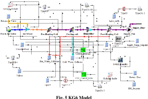
The final KG6 TRNSYS model is represented by the following figure:

Fig. 5 KG6 Model

KG7 is not presented here but it is almost the same model. On the last figure we can recognize the different components that we defined in the previous section. Here is a short explanation of the main components based on the Mathematical reference user guide of TRNSYS as well as the TESS documentation.

The air mixer component (TYPE 648) is responsible of mixing the return air coming from the offices with the fresh outside air. The pressure drop across the mixer is supposed to be zero. The model is based on a simple mass balance.

(5)

The pre-heating coil (and post-heating coil) is modelled by a simple heating coil (TYPE 753) with air by-pass factor approach. This pre-heating coil works in free-floating mode or uncontrolled mode in the sense that we control the inlet water flow rate by ourselves outside the coil model.

The only parameter that we can use to describe the efficiency of the coil is the by-pass factor f_bypass. In this model, the coil is supposed to have an efficiency of 100% for a given by-pass factor. If there is no trivial solution - zero flow, inlet water temperature lower than inlet air temperature… - an iterative process computes the outlet conditions by balancing the energy removed from the air stream with the energy added to the fluid stream.

First of all, an outlet water temperature Tguess is guessed. We assumed that the outlet air exits the coil at the coil water average temperature:

2 out water in water avg water T T T   . (1)

Knowing the outlet air conditions, we can compute the energy transferred to the air by the water:







in



air out air bypass air water m f h h Q   1  . (2)

The outlet water temperature is then determined by the following equation:

water p water water in water out water c m Q T T     , ₍₃₎

where cp_water is the mass-specific heat capacity of the water.

The water cannot exit the coil at a temperature lower than the temperature of the inlet air. If this condition is not respected, the outlet water temperature is set equal to the inlet air temperature and the energy is recalculated as follow:



in



air in water water p water water m c T T Q    . (4)

As the energy removed from the water must be equal to the energy added to the air stream, we can deduce the enthalpy of the outlet air:



bypass



air water in air out air f m Q h h    1   . (5)

The humidity ratio is not supposed to vary during the heating process. The outlet air conditions are then completely determined at this point. If the last computed outlet water temperature is not too far from the guessed temperature, the process has converged. In other words, the process reaches an end when the following condition is fulfilled:



 guess



 out

water T

T

abs , (6)

where  is a small value, typically around 0.01. If the condition is violated, the iterative process continues with a new guess until convergence is reached. The new guess is computed as follow: 4 old guess out water old guess new guess T T T T    . (7)

(6)

Once the process has converged, the outlet air stream is then mixed with the by-pass air stream and the model has finally completed its calculations.

The method of calculation in the model of cooling coil (TYPE 508) looks like the one for the heating coil. The difference lies in the fact that dehumidification is to be considered. The moisture lost by the air stream exits the coil as a condensate flow rate. It is assumed that the air exits the coil at the average water temperature of the coil. As it is difficult to calculate the heat transfer between the air and the coil because the coil tubes are usually wet with condensation, the model splits the air flow into two parts:

- the first part of the air flow passes through the coil and exits in saturated condition at the temperature of the coil water,

- the second part is by-passed around the coil and is then remixed with the other part which passed through the coil.

As we need the average water temperature in the coil and we do not know the outlet water temperature, this one is guessed and adapted at each iteration until the energy removed from the air matched the energy added to the water. The condensate flow can then be found by







in



air out air bypass air condensate m f m   1   , (8)

where f_bypassis the by-pass factor of the air. The energy transferred from the air to the water is:







condensate condensate out air in air bypass air water m f h h m h Q   1    , (9)

where hcondensate is the enthalpy of the condensate found by the TRNSYS Steam properties routine.

The new outlet water temperature is finally given by:

water p water water in water out water c m Q T T     . ₍₁₀₎

Once the iterative process has converged, the flow of air exiting the coil is remixed with the by-passed air flow rate to give the final outlet conditions.

The adiabatic humidifier model is based on an energy balance (TYPE 641). We assume that the water temperature is not affected by the air conditions during the process which means thatT_waterout T_waterin . The model first supposes that the flow rate of condensate is zero. We can thus write the energy balance on the humidifier as follow:

in water air in water in air out air h m m h h     . (11)

We can determine the outlet air humidity ratio thanks to the mass balance:

air in water in air out air m m      . (12)

Knowing the outlet conditions we can check the air for saturation. If the air has passed the saturation point, we set the air properties to its saturated conditions. The model then recalculates the energy balance taking the flow rate of condensate into account:

(7)

8th International Conference on System Simulation in Buildings, Liege, December 13-15, 2010 out water air out water in water air in water in air out air h m m h m m h h        , (13)

where h_waterout is calculated assuming T_waterout T_waterin . Finally the new enthalpy of the outlet air is compared to the enthalpy of the last iteration. If the difference falls below a tolerance of 0.01kJ/kg.K, then the process terminates.

The fan model used is the TYPE 111 of TRNSYS. The power of the fan is computed as follow:







 _ _ _ _ 3_ 3 2 2 1 0 a a  a  a P P rated , (14)

where Prated is the rated power and σ is the fan control signal which is 0 if the fan is off (in this case, the power is set to 0), 1 if the fan works at full speed or a linear value between 0 and 1 if the fan is operating at an intermediate speed. The flow rate of air passing through the fan is then given by the following linear relationship m m_rated where m_rated is the rated flow rate. The coefficients ai and the degree of the normalized polynomial curve depend on the fan

and have to be given by the user.

3.2 Control

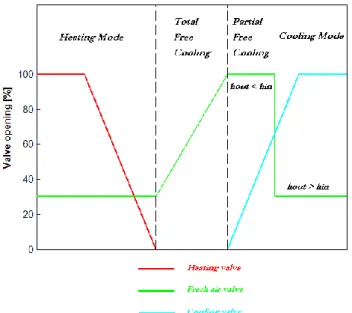
The supply air temperature and humidity are controlled via the post-heating coil and the humidifier with simple PI controllers. The most difficult part of the control concerns the behaviour of the economizer, the pre-heating coil and the cooling coil in order to reach the set point after the humidifier. This is a sequential control of operations as shown on the following figure:

Fig. 6 Control scheme for economizer, pre-heating valve and cooling valve

If we have a heating need, the pre-heating water valve is opened while the fresh air valve is closed at its minimum value (30%). Once the heating valve is fully closed, it means we have a cooling need. Then the total free cooling mode is turned on with the opening of the fresh air valve. If the fresh air valve reaches its maximal opening and if the cooling need is not satisfied, then the cooling coil valve opens while the fresh air valve remains fully opened.

(8)

This is what we call the partial free cooling mode because the cooling energy is provided by both the outside air and the battery.

When the outside air is not appropriate for cooling because it is for example hotter than the inside air, the fresh air valve must close to its minimum. This appears if the enthalpy of the outside air is greater than the enthalpy of the inside air. When this enthalpy condition is fulfilled the total cooling mode is operating.

In order to reach the set point of temperature after the humidifier we need to know if we are in heating, free cooling or cooling mode. Each of these modes has a PI controller to control the heating water valve, the fresh air valve and the cooling water valve.

At a particular time step we do not know the amount of fresh air that will be added and the decrease of temperature due to the humidifier when it is turned on. So we can not predict if it is the pre-heating coil, the fresh air valve or the cooling coil that will have to work. The way to find which mode is active is to simulate each mode separately and choose the one that gives the right answer, that is to say the solution that reaches the set point of temperature. Simulating the 3 modes at each time step is a lot of calculation because 3 PI controllers are working at the same time. If we choose a time step small enough then we can consider that the mode of the previous time step is still active at the current time step except if the set point can not be reached anymore. The control strategy that we implemented is the following:

1) When the system is turning on for the first time in the morning, the 3 modes are simulated which means that the 3 PI controllers are working together. The controller that gives the smaller error wins and the corresponding mode is chosen. The error is calculated as the absolute difference between the temperature after the humidifier and the set point after the humidifier.

2) If the system is running during the day, the mode of the previous time step is still active until the set point cannot be reached. If there is a change of mode, different cases can occur:

a) If it was in heating mode at the previous time step and if the heating valve solution given by the controller is 0% then the free cooling mode is activated.

b) If it was in free cooling mode at the previous time step, then if the fresh air valve control signal is 0%, the heating mode is activated. If the fresh air valve signal reaches 100%, then the partial free cooling mode is activated. c) If the partial free cooling mode was activated at the previous time step, then

if the cooling valve control signal falls down to 0%, the free cooling mode is activated. Otherwise if the enthalpy condition hout<hin is violated, then

the fresh air valve is closed at minimal opening and the total cooling mode is activated.

d) If the total cooling mode was activated at the previous time step, then when the enthalpy condition is respected again, the partial free cooling mode is turned on.

3.3 Integrated building-system model

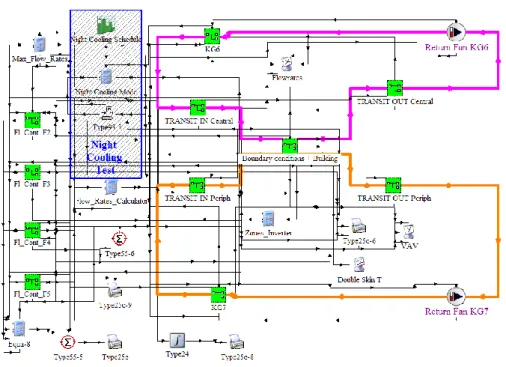
Once the KG6 and KG7 models were ready, we integrated the system model with the building model. The global TRNSYS model is presented on the following figure:

(9)

Fig. 7 Integrated building-system model

The pink line represents the air network treating by the KG6 unit. The VAV boxes (F1_Cont_F2, F1_Cont_F3, F1_Cont_F4 and F1_Cont_F5) are simple equations that compute the percentage of VAV openings depending on the offices temperature.

Fig.8 VAV boxes control

The VAV boxes modulate the flow rate of air entering the offices. If all the VAV boxes are opened at 100% when it is too hot or too cold in the offices then the fans will work at maximal power and the flow rate will be maximal.

On Fig.7, the orange line represents the air network of the KG7. The blue rectangle is composed by some additional elements to simulate a night cooling scheme according to the wish of the user.

One important assumption is made here. The building offices, composed by the inner sector and outer sector as we described above, were modelled by only one zone per floor in TRNSYS. In fact it is supposed that the thermal behaviour of the inner sector is approximately the same than the outer sector which is not a bad approximation. In

(10)

consequences the KG6 system supplies the air in the TRNSYS zone and extracts it from the zone in the model while the KG7 supplies the air in the same zone and extracts it from the double skins zones. It also means that we have modelled only one VAV box per zone because we have only one temperature available per zone. The percentage of maximal flow rate for both air-handling units will then be the same.

The integrated building-system simulation is a really big simulation. In fact the maximum number of outputs allowed by TRNSYS was exceeded. Therefore we had to increase this constant in the TRNSYS Fortran source code and recompile the software to be able to run the simulation.

To insure the convergence of the simulation and to avoid oscillations from the controllers the time step was decreased to a value of 1 minute. The consequence is a greater calculation time. One yearly simulation takes about 4 hours 30 minutes to run! This time can be longer depending on the processor of the computer used.

4 CALIBRATION OF THE MODEL

4.1 Instrumentation

In order to calibrate the system model a monitoring campaign took place in winter 2010 for a period of 3 months (January, February and March). This session was divided in two parts. The first part in January consisted in collecting the measurements to calibrate the model. After this first session we applied some improvements to the system and start another monitoring session. The set of these new measurements is used to validate the calibration of the model. Only KG7 was calibrated. Some sensors were also placed on KG6 but as we only have two flow meters available it was not possible to get any information about the water network of KG6. Moreover the measurements on KG6 showed some inaccuracies from the BEMS sensors. We decided then to focus on KG7.

The measurements points are summarized on the following graph:

Fig. 9 KG7 measurement points

We placed a temperature-humidity sensor in the mixing chamber before the filter to measure the temperature and humidity of the mixture between the return air and the fresh air. If we know the flow rate we can deduce the percentage of added fresh air from the temperatures of the return air and outside air.

To have an idea about the heating consumption an ultrasonic flow meter was installed on both the pre-heating coil and post-heating coil to measure the flow rate of water entering the batteries. Surface temperature sensors are responsible of measuring the temperature of the inlet water and outlet water of both batteries.

(11)

The air temperature after the pre-heating coil was not measured because it was not possible to reach this point without making holes in the wall of the pipe.

On the other hand the temperature of the air after the humidifier was measured as well as the temperature and humidity of the air after the post-heating coil but before the supply fan. The air temperature and humidity after the supply fan is given by the BEMS. The validity of this BEMS sensor was checked. We can thus trust this value. The power consumption of the supply fan was measured by a power meter during all the session.

The last temperature-humidity sensor is placed before the KG7 return fan to measure the temperature and humidity of the return air. This sensor is autonomous which means that it can save the measurements data by itself while the other sensors we installed were all linked to a data acquisition unit.

4.2 Calibration approach

The first step of the calibration is to define the part of the model that will be calibrated as well as the inputs we give to this segment of model and the output we want to compare to the reality. Then we have to define the parameters that will be adapted so that the simulation matches as best as possible the measurements we made.

In our case we want to calibrate the KG7 system. The calibration segment of model includes all the KG7 system from the return-fresh air mixing chamber to the supply fan. The return fan is not calibrated because we have no measurements about it.

Although we have power measurements on the supply fan it is not possible to calibrate it. Indeed the flow rate of supply air is partially defined by the VAV boxes. If we know the behaviour of the VAV boxes we can thus deduce the flow rate and then the power of the fan that we can compare to measurements. Unfortunately the BEMS can not provide any information about the VAV. It implies that the real control of the supply fan is not well determined and that we can thus not calibrate the parameters of the fan. The power of the supply fan is then chosen as an input of the model.

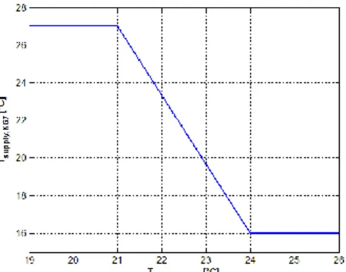
The other inputs are the outside air conditions (temperature and humidity) given by the BEMS and the return air conditions measured by our sensors. The supply air set point noticed on site was:

Fig. 10 KG7 Supply air set point during calibration

We decided to calibrate the model on a period of one week. The parameters that we calibrate are the by-pass factor of the pre-heating coil, the humidifier moisture rate and the by-pass factor of the post-heating coil. The cooling coil is not calibrated because the monitoring session took place in winter when the coil is all the time turned off.

(12)

During the calibration job some additional assumptions were made. After carefully looking at the measurements we noticed that the humidifier turns on when the humidity in the return duct is less than approximately 38.5% and turns off when it is more than 46%. Remembering that the set point is normally the interval [40, 60] % we changed it to match the real behaviour. The last change we made is adapting the working schedule of the system. The measurements show that the system turns on at 7am and turns off at 6pm during the week days. During the weekend the system is supposed to be turned off.

4.3 Calibration Results

The calibration parameters that we found are: pre-heating coil by-pass factor: 0.9, humidifier moister rate: 146.23 kg/h, post-heating coil by-pass factor: 0.73.

The comparison between some simulation result curves and the measurement curves is presented below with different graphs. In red we have the measurements, in blue the simulation results. The calibration was made only for the day period during which the system is turned on.

The following graph is the comparison between the temperature after the humidifier of the simulation and the one measured. We can see a rather good correspondence.

0.00 5.00 10.00 15.00 20.00 25.00 30.00 0 24 48 72 96 120 144 Time [h] T [ °C ] THumidiferKG7_simulation THumidiferKG7_measure

Fig. 11 Comparison between simulation and measurements (T after humidifier) The graph below is the comparison for the temperature after the post-heating coil. The two curves match well for the 3rd and 4th day but the result is a bit worst for the other days especially in the morning. We can not really explain this difference; all we can say is that it is maybe due to the control of the BEMS which is not perfect and maybe worst than the one of the simulation. Anyway the difference that we observe is about only 1°C which is a good result. 0.00 5.00 10.00 15.00 20.00 25.00 30.00 0 24 48 72 96 120 144 Time [h] T [ °C ] TPostHeatKG7_simulation TPostHeatKG7_measure

(13)

The next graph is the comparison concerning the relative humidity after the post-heating battery. Here again the error is only some percents of humidity.

0.00 20.00 40.00 60.00 80.00 100.00 0 24 48 72 96 120 144 Time [h] R H [ % ] RHPostHeatKG7_simulation RHPostHeatKG7_measure

Fig. 13 Comparison between simulation and measurements (RH after post-heating coil) The last graph is a comparison between the supply temperature found by simulation and the one given by the BEMS system. There is also a small difference here because we already had a difference for the previous temperature. The BEMS curve confirms that there is a kind of offset made by the BEMS because the supply temperature reaches 29°C although the maximum supply temperature defined in the BEMS and also in the simulation was 27°C.

0.00 5.00 10.00 15.00 20.00 25.00 30.00 0 24 48 72 96 120 144 Time [h] T [ °C ] TSupplyKG7_simulation TSupplyKG7_Siemens

Fig. 14 Comparison between simulation and BEMS (T supply)

As we are interested to match the real heating consumptions, we can compare the one given by the simulation to the consumption measured on site. The following table shows this comparison as well as the percentage of error.

Table 1: Comparison between simulation and measurements (Heating Consumption)

Pre-heating (kWh) Post-heating (kWh)

Simulation 3621.59 4319.61

Measurements 3745.83 4295.83

Difference 3.32% -0.55%

As you can see the errors are rather small which tends to prove that the model matches the reality well.

4.4 Validation

The second part of the monitoring session is used to validate the calibration. The period of validation is one week. We apply the improvements made on site to the calibrated model and run a weekly simulation with the inputs corresponding to the validation week. Two improvements were made on KG7:

(14)

I. Control of the fresh air valve in function of the CO2 in the offices (with a minimal fresh air valve opening of 0%). The set point is 800ppm although we ask the building team for 1000ppm.

II. Change of the supply temperature set point to:

Fig. 15 KG7 supply air set point during validation

The idea of the first improvement is to reduce the use of cold fresh air in order to decrease the heating consumption. Reducing the amount of fresh air is permitted because the CO2

-concentration is never greater than 700ppm in the offices as shown by a CO2 measurements

session realized by the University of Gent.

During the monitoring session the CO2 concentration was measured by the BEMS building

team. Unfortunately they did not provide us these measurements although we asked them by mail. As we need to include a CO2 model in our simulation we decided to use the CO2

measurements given by the University of Gent over a period of one day to fit our model. We know that the fresh air valve opening is at a minimum of 30% for this day. The following graph shows the comparison between our CO2 model in blue and the CO2-concentration in red.

0 100 200 300 400 500 600 700 800 0:00 2:30 5:00 7:30 10:00 12:30 15:00 17:30 20:00 22:30 Time C O 2 [ p p m ] CO2measure CO2model

Fig. 16 Comparison between model and measurements (CO2) The model is a simple mass balance equation:



m m m



t m m S k CO Fresh CO k CO k CO       _ _ _ 2 2 2 2 1 , (15) Where - m_COk

2 is the mass of CO2 in the total office zone at time k (mg),

- m_COFresh

2

 the mass flow rate of CO2 coming from the outside air and entering in the total office

zone (mg/h), - m_COk

2

(15)

- mS the CO2 mass source in [mg/h], - t the simulation time step.

The CO2 rate in the offices is calculated as follow:

V m t COk k CO 44 4 . 22 1 1 2 2   _ .

V is the volume of the office zone (outer sector), 22.4 [l/mole] the molar volume of any gas assumed perfect and 44 [g/mole] the molar mass of the CO2.

The CO2 mass source can be written as mS S Vt 4 . 22

44 

 where S is the CO2 source in

[ppm/h]. The model has thus two parameters which are the CO2 concentration of the outside

air and the sourceS. The calibration results are 400ppm for the outside air and (425*f)ppm/h for the source with f a schedule function that takes the fact into account that all people do not arrive and leave the building at the same time and that they go out every day for having lunch. In the model we assume that the CO2 concentration in the offices is equal to the outside air CO2 concentration during the night and during the weekend.

4.5 Validation Results

After analysing the mixing temperature results we noticed that the minimum of fresh air when the CO2 is less than 800 ppm was not 0 but 20% of the maximal flow rate. We can not

clearly explain this. Maybe the team responsible of the building changed what we defined or maybe there is a hardware limit to the minimum fresh air opening.

The validation results are shown below on different graphs. We observe a rather good correspondence between the measurements and the simulation outputs on each graph.

0.00 5.00 10.00 15.00 20.00 25.00 30.00 0 24 48 72 96 120 144 Time [h] T [ °C ] THumidiferKG7_simulation THumidiferKG7_measure 0.00 5.00 10.00 15.00 20.00 25.00 30.00 0 24 48 72 96 120 144 Time [h] T [ °C ] TPostHeatKG7_simulation TPostHeatKG7_measure

(16)

8th International Conference on System Simulation in Buildings, Liege, December 13-15, 2010 0.00 10.00 20.00 30.00 40.00 50.00 60.00 70.00 80.00 90.00 100.00 0 24 48 72 96 120 144 Time [h] R H [ % ] RHPostHeatKG7_simulation RHPostHeatKG7_measure 0.00 5.00 10.00 15.00 20.00 25.00 30.00 0 24 48 72 96 120 144 Time [h] T [ °C ] TSupplyKG7_simulation TSupplyKG7_Siemens

Fig. 17 Comparison between simulation and measurements (Validation week)

At the level of the heating consumptions we can see on the following table that the error is less than 10%.

Table 2: Comparison between simulation and measurements (Heating Consumption)

Pre-heating (kWh) Post-heating (kWh)

Simulation 3317.25 2464.66

Measurements 3065.83 2578.64

Difference -8.20% 4.42%

5 IMPROVEMENT OF THE SYSTEM PERFORMANCE

Here is below the simulation results sheet for a yearly simulation run with the same set points and control than the calibration simulation that is to say with the system not improved. We divided the results into two parts, one for KG6 and one for KG7. For each air-handling unit, we give the electrical consumption of the fans, the humidifier pump and the cooling coil. Moreover we provide the consumption of the pre-heating coil and post-heating coil. All of these consumptions are given in kWh. The average flow rate and the minimum flow rate in m³/h as well as the humidifier water consumption in m³ are also given.

For economical information we calculate the cost of each energy consumption. We assumed the following prices:

 electricity during the day: 0.1063 €/kWh,  electricity during the night: 0.0664 €/kWh,  gas: 0.03113 €/kWh.

(17)

In the last column we provide the primary energy used in kWh. The conversion factors for primary energy are the following:

 electricity conversion factor: 2.5,  gas conversion factor: 1.1.

At the end of the sheet we also give the average VAV openings for each floor during the period of the time tested.

As we can see in the table the total cost is about 17257 € for the reference simulation. Table 3: Result sheet (Reference case)

Period: Year

Cost (€) Primary Energy (kWh)

KG6 Supply Fan Consumption (kWh) 3637.19 386.63 9092.98 Return Fan Consumption (kWh) 2425.85 257.87 6064.62

Max flow rate (m³/h)

30198 Pre-Heat (kWh) 49816.57 1550.79 54798.23 Min Fresh Air valve Cool (kWh) (Latent: 19.06 %) 5329.57 566.53 13323.92 0.3 Humidifier (kWh) 303.84 32.30 759.59 Post-Heat (kWh) 88801.09 2764.38 97681.19

Average Flow Rate (m³/h) 13492.66 Minimum Fresh Air Flow Rate (m³/h) 9059.40 Humidifier Water Consumption (m³) 48.04

5558.50 181720.53

60931 Pre-Heat (kWh) 132828.22 4134.94 146111.04 Min Fresh Air valve Cool (kWh) (Latent: 19.87 %) 7782.35 827.26 19455.88 0.3 Humidifier (kWh) 284.97 30.29 712.42 Post-Heat (kWh) 164346.36 5116.10 180781.00

11698.84 384460.15 Total (€): 17257.34 566180.69

Average VAV openings (%)

- FLOOR2 41.50%

- FLOOR3 37.67%

- FLOOR4 38.12%

(18)

The second test is run with the improved system of the validation week. The supply air set point is changed and we add the CO2-concentration control with a minimum fresh air valve

opening of 20%. The improvement of the cost is almost 30%! A big part of the improvement is of course due to the reduction of the heating consumption especially the post-heating consumption. If we use less fresh air with a carbon dioxide control then the heating consumption decreases.

Table 4: Result sheet (improved case)

Period: Year, Improved

30198 Pre-Heat (kWh) 39313.82 1223.84 43245.20 Min Fresh Air valve Cool (kWh) (Latent: 18.70 %) 4662.45 495.62 11656.13

0.2 Humidifier (kWh) 238.66 25.37 596.64

Post-Heat (kWh) 61135.90 1903.16 67249.49

4092.80 133208.71

60931 Pre-Heat (kWh) 110796.25 3449.09 121875.88 Min Fresh Air valve Cool (kWh) (Latent: 19.11 %) 6284.06 668.00 15710.15

0.2 Humidifier (kWh) 267.87 28.47 669.67

Post-Heat (kWh) 101819.14 3169.63 112001.05

8412.72 276068.82 Total (€): 12505.52 409277.54 % -27.54% -27.71%

Average VAV openings (%)

- FLOOR2 35.73%

- FLOOR3 33.62%

- FLOOR4 34.30%

(19)

Having a great improvement is nice but what about the comfort in the offices? To have an idea about this we ran a simple comfort calculation with TRNSYS for the basic simulation and for the simulation with an improvement of 54%. For simplicity we used a constant clothing factor of 1.2. First we consider only a winter period. The following histograms show the number of hours during which the PMV value is included in a certain interval for each floor of the building. The intervals chosen are [-1.5, 1], [-1,-0.5], [0, 0.5], [0.5, 1] and [1, 1.5]. It is usually considered to be comfortable when the PMV value is between -0.5 and 0.5.

Fig. 18 Comfort comparison for a winter period (basic case to the left and improved case to the right)

We can see that the comfort is not worst with the improvements we added, it is even better for the floor 5. Note that the floor 5 tends to be colder than the other ones. The control of this floor should be then different.

Now we consider the same analysis but for a yearly period.

Fig.19 Comfort comparison for a yearly period (basic case to the left and improved case to the right)

We can note that in this case the comfort is worst in each floor. Although we have an improvement in cost of 30% and although the comfort is still good in winter unfortunately the comfort is deteriorated in hotter season. The improvements chosen are good for winter season and will bring a great benefit but other set points should be chosen when the climate implies that we have to cool the building. Reducing the cost of consumption of a system sometimes goes with deteriorating the comfort. The job of trying to optimize the cost should always be done with a comfort study in parallel.

(20)

6 CONCLUSION

This paper demonstrates the advantages and the disadvantages of using a simulation tool in relationship with a BEMS. We could see how difficult the implementation of an integrated building-system model was if we use dynamic simulation and if we go deep in details into the model. This work takes a lot of time to be realized and the computation time and complexity of the simulation due to complex control can become rather big. Remember that we focus on only one building with its system.

Another difficulty concerns the calibration of the model which requires a monitoring campaign. This kind of job is difficult to achieve because you have to be sure about the measured values given by the sensors. The measurements can be wrong if the sensors encounter troubles or if the position of the sensors is not correct. In this case the calibration can become a hard job. Moreover we realized that it was difficult to deal with the team responsible of the building which does not always agree with the changes you want to apply to the system.

Nevertheless the simulation allowed us to bring to light some failing BEMS sensors. The simulation is thus a good tool for faults detection of BEMS systems.

Finally we showed that the simulation tool can be used to improve the system consumption and thus the total cost paid by the building users. In our case we reached an improvement of 27% at the cost level just by changing some control set points and by adding a CO2 control in

the offices. The investment is not more than a few thousands euros for CO2 sensors.

Therefore the payback time is less than one year for this case study. Remember that this improvement is effective for the climate and shading we tested and that the behaviour of the system can completely changed depending on the location. The use of a simulation tool can thus not be generalized to any building and systems but should remain useful for a particular case only.

NOMENCLATURE avg

water

T Coil water average temperature mcondensate Condensate flow rate

in water

T Inlet water temperature (coil and humidifier) h_airin Inlet air enthalpy

out water

T outlet water temperature (coil and

humidifier)

out air

h Outlet air enthalpy

air

m Air flow rate T_guess Guessed temperature

water

m Water flow rate in

air

 Inlet air humidity ratio

condensate

h Condensate enthalpy out

air

 Outlet air humidity

ratio REFERENCES

Solar Energy Laboratory, University of Wisconsin-Madison, 2007, TRNSYS 16 Volume 4

Mathematical Reference.

University of Liège, University of Gent, Guangzhou Institute of Energy Conversion, 3E, 2010, Joint Sino-Belgian project on energy savings in buildings by combined dynamic