The CARMENES search for exoplanets around M dwarfs. Two planets on opposite sides of the radius gap transiting the nearby M dwarf LTT 3780

Astronomy

_&

Astrophysics

© ESO 2020

The CARMENES search for exoplanets around M dwarfs

Two planets on opposite sides of the radius gap

transiting the nearby M dwarf LTT 3780

G. Nowak

_{, R. Luque}

_{, H. Parviainen}

_{, E. Pallé}

_{, K. Molaverdikhani}

_{, V. J. S. Béjar}

_{, J. Lillo-Box}

_,

C. Rodríguez-López

_{, J. A. Caballero}

_{, M. Zechmeister}

_{, V. M. Passegger}

_{, C. Cifuentes}

_{, A. Schweitzer}

_,

N. Narita

_{, B. Cale}

_{, N. Espinoza}

_{, F. Murgas}

_{, D. Hidalgo}

_{, M. R. Zapatero Osorio}

_{, F. J. Pozuelos}

_,

F. J. Aceituno

_{, P. J. Amado}

_{, K. Barkaoui}

_{, D. Barrado}

_{, F. F. Bauer}

_{, Z. Benkhaldoun}

_{, D. A. Caldwell}

_,

N. Casasayas Barris

_{, P. Chaturvedi}

_{, G. Chen}

_{, K. A. Collins}

_{, K. I. Collins}

_{, M. Cortés-Contreras}

_,

I. J. M. Crossfield

_{, J. P. de León}

_{, E. Díez Alonso}

_{, S. Dreizler}

_{, M. El Mufti}

_{, E. Esparza-Borges}

_{, Z. Essack}

_,

A. Fukui

_{, E. Gaidos}

_{, M. Gillon}

_{, E. J. Gonzales}

, P. Guerra

, A. Hatzes

, Th. Henning

, E. Herrero

,

K. Hesse

_{, T. Hirano}

_{, S. B. Howell}

_{, S. V. Jeffers}

_{, E. Jehin}

_{, J. M. Jenkins}

_{, A. Kaminski}

_{, J. Kemmer}

_,

J. F. Kielkopf

_{, D. Kossakowski}

_{, T. Kotani}

_{, M. Kürster}

_{, M. Lafarga}

_{, D. W. Latham}

_{, N. Law}

_,

J. J. Lissauer

_{, N. Lodieu}

_{, A. Madrigal-Aguado}

_{, A. W. Mann}

_{, B. Massey}

_{, R. A. Matson}

_{, E. Matthews}

_,

P. Montañés-Rodríguez

_{, D. Montes}

_{, J. C. Morales}

_{, M. Mori}

_{, E. Nagel}

_{, M. Oshagh}

_{, S. Pedraz}

_,

P. Plavchan

_{, D. Pollacco}

_{, A. Quirrenbach}

_{, S. Reffert}

_{, A. Reiners}

_{, I. Ribas}

_{, G. R. Ricker}

_{, M. E. Rose}

_,

M. Schlecker

_{, J. E. Schlieder}

_{, S. Seager}

_{, M. Stangret}

_{, S. Stock}

_{, M. Tamura}

_{, A. Tanner}

_{, J. Teske}

_,

T. Trifonov

_{, J. D. Twicken}

_{, R. Vanderspek}

_{, D. Watanabe}

_{, J. Wittrock}

_{, C. Ziegler}

_{, and F. Zohrabi}

(Affiliations can be found after the references) Received 2 March 2020 / Accepted 17 July 2020

ABSTRACT

We present the discovery and characterisation of two transiting planets observed by the Transiting Exoplanet Survey Satellite (TESS) orbiting the nearby (d?≈ 22 pc), bright (J ≈ 9 mag) M3.5 dwarf LTT 3780 (TOI–732). We confirm both planets and their

associ-ation with LTT 3780 via ground-based photometry and determine their masses using precise radial velocities measured with the CARMENES spectrograph. Precise stellar parameters determined from CARMENES high-resolution spectra confirm that LTT 3780 is a mid-M dwarf with an effective temperature of Teff= 3360 ± 51 K, a surface gravity of log g?= 4.81 ± 0.04 (cgs), and an iron

abundance of [Fe/H] = 0.09 ± 0.16 dex, with an inferred mass of M?= 0.379 ± 0.016 Mand a radius of R?= 0.382 ± 0.012 R. The

ultra-short-period planet LTT 3780 b (Pb = 0.77 d) with a radius of 1.35+0.06_−0.06R⊕, a mass of 2.34+0.24−0.23M⊕, and a bulk density of

5.24+0.94

−0.81g cm−3joins the population of Earth-size planets with rocky, terrestrial composition. The outer planet, LTT 3780 c, with an

orbital period of 12.25 d, radius of 2.42+0.10

−0.10R⊕, mass of 6.29+0.63−0.61M⊕, and mean density of 2.45+0.44−0.37g cm−3belongs to the population

of dense sub-Neptunes. With the two planets located on opposite sides of the radius gap, this planetary system is an excellent target for testing planetary formation, evolution, and atmospheric models. In particular, LTT 3780 c is an ideal object for atmospheric studies with the James Webb Space Telescope (JWST).

Key words. techniques: photometric – techniques: radial velocities – stars: individual: LTT 3780 – stars: late-type – planets and satellites: detection

1. Introduction

In a sequence of space-based transit surveys that commenced with the CoRoT mission (Auvergne et al. 2009) and continued with Kepler (Borucki et al. 2010) and K2 (Howell et al. 2014), the Transiting Exoplanet Survey Satellite (TESS; Ricker et al. 2015) is the first to cover nearly the entire sky in a search for transiting planets. This includes 2 min short-cadence monitor-ing of almost all M dwarfs brighter than 15 mag in the TESS bandpass. Based on Kepler results, Dressing & Charbonneau

(2013) showed that planets with radii below 4 R⊕ are almost

?_{National Science Foundation Graduate Research Fellow.}

the only type of planets orbiting M dwarfs. Planetary systems around bright TESS red dwarfs are therefore optimal laborato-ries for testing formation, evolution, and interior models of small planets (Rp∈ 1–4 R⊕) that have no known counterparts in the

Solar System. Detailed characterisation of small planets orbiting bright M dwarfs also allows optimal candidates to be selected for future in-depth atmospheric studies (see e.g.Snellen et al. 2013;

Batalha et al. 2018).

As was shown byFulton et al.(2017) andFulton & Petigura

(2018), the radius distribution of small, close-in planets (with orbital periods P < 100 d) has a bi-modal structure with a gap around 1.7 R⊕that separates the two main classes of small

8400 8600

Rel. Flux

Simple Aperture Photometry (SAP)

8800 8900 9000 Rel. Flux PDC-corrected SAP 8545 8550 8555 8560 8565 BJD - 2450000 (d) 0.99 1.00 1.01 Rel. Flux Custom SAP

Fig. 1.TESS data of LTT 3780. Top panel: simple-aperture photometry from SPOC pipeline. Middle panel: PDC-corrected photometry from SPOC pipeline. Bottom panel: custom-aperture photometry as inHidalgo et al.(2020). Blue and orange ticks below the light curve mark the transits of the candidates TOI–732.01 (blue) and TOI–732.02 (orange). Red ticks above the light curves mark two dips that might correspond to single-transit events.

and gas-dominated sub-Neptunes with radii centred at 2.4 R⊕.

For planets orbiting the same star, and hence exposed to the same irradiation, differences in the planetary bulk densities and atmospheric structures could then be mainly explained by dif-ferences in their masses and orbital distance. Planetary systems with two or more close-in, small planets located below and above the radius gap are therefore especially interesting for study-ing the formation, evolution, and atmospheric composition of small planets. So far only a few such systems have been char-acterised in terms of precise radii measured with space-based transit telescopes and masses determined via high-precision radial velocity (RV) measurements. These systems are: Kepler-10 bc (Dumusque et al. 2014), K2-106 bc (Sinukoff et al. 2017;

Guenther et al. 2017), HD 3167 bc (K2-96 bc; Christiansen et al. 2017; Gandolfi et al. 2017), GJ 9827 bcd (K2-135 bcd;

Niraula et al. 2017; Prieto-Arranz et al. 2018), K2-138 bcdef (Christiansen et al. 2018; Lopez et al. 2019), HD 15337 bc (TOI-402 bc;Gandolfi et al. 2019;Dumusque et al. 2019), and K2-36 bc (Damasso et al. 2019).

Here, we present the discovery of two transiting TESS plan-ets straddling the radius gap around the nearby, bright M dwarf LTT 3780. Given the brightness of the host star, these plan-ets are suitable for detailed atmospheric characterisation with future ground- and space-based facilities. The paper is structured as follows: Sect. 2 presents the analysis of TESS photometry used for the discovery of planets around LTT 3780. In Sect. 3, ground-based observations of LTT 3780 are presented, includ-ing seeinclud-ing-limited transit photometry, high-resolution imaginclud-ing, and high-resolution spectroscopy with CARMENES. Detailed analyses of the stellar properties of LTT 3780 are presented in Sect.4, while Sect.5presents the joint analysis of all available data and the derived planetary properties. Finally, a discussion and conclusions are presented in Sects.6and 7.

2. TESS photometry

2.1. Space-based observations

LTT 3780 (TOI–732, TIC 36724087) was observed by TESS in short cadence mode (2-min integrations) during cycle 1, sector 9 (camera #1, CCD #1) between 28 February and 25 March 2019, and it is expected to be observed again during the first year of the extended mission (cycle 3), sector 35 (camera #1) between 9 February and 7 March 2021. In total, 21.736 days of science data

were collected for LTT 3780. The 1.182-day gap in the TESS photometry between BJDTDB= 2 458 555.54677 and BJDTDB=

2 458 556.72869 was caused by the data download dur-ing perigee passage. Data collected between BJDTDB=

2 458 543.22185 and BJDTDB= 2 458 544.43991 (1.218 day)

and between BJDTDB= 2 458 556.72869 and BJDTDB=

2 458 557.85228 (1.123 day) were excluded from the light curves of all targets on Camera #1 CCD #1 because of the strong scattered light at the beginning of orbits 25 and 26 that was problematic for systematic error correction and the subsequent transiting planet search.

2.2. Transit search

We downloaded from the Mikulski Archive for Space Telescopes1 _{(MAST) the corresponding TESS light curve of} LTT 3780 produced by the Science Processing Operations Center (SPOC;Jenkins et al. 2016) at the NASA Ames Research Cen-ter. For this target, SPOC provided simple aperture photometry (SAP;Twicken et al. 2010;Morris et al. 2017) and systematics-corrected photometry, a procedure consisting of an adaptation of the Kepler Pre-search Data Conditioning algorithm (PDC;

Smith et al. 2012;Stumpe et al. 2012,2014) to TESS. The SPOC light curves generated by both methods are shown in the first two panels of Fig.1.

Additionally, we retrieved the TESS target pixel file (TPF) from MAST and performed a custom selection of pixels to build the optimal aperture that maximises the transit signals in the light curve (see Sect.2.3). Following the methods described in

Hidalgo et al.(2020), we used our own analysis pipeline based on the everest2 _{pipeline (Luger et al. 2016,2018), which applies} the pixel level decorrelation (PLD) technique (Deming et al. 2015) to extract from the raw light curve a final, flattened version (see bottom panel in Fig.1). To detect possible transit events, we used the box-fitting least squares (BLS) algorithm (Kovács et al. 2002) on the flattened light curve to search for periodic sig-nals. Once a signal was detected, we modelled the transit with batman(Kreidberg 2015) and removed it from the light curve. We iteratively used this procedure until no further signals were detected. We found two periodic signals at 0.7685 ± 0.0007 and

1 _{https://mast.stsci.edu/portal/Mashup/Clients/Mast/} Portal.html

332 334 336 338 340 342

Pixel Column Number

1578 1580 1582 1584 1586 1588

Pixel Row Number

E N

TOI-732 (TIC 36724087) - Sector 9

m = -2.0 m = 0.0 m = 2.0 m = 5.0 m = 8.0 1 2 3 4 5 6 7 8 9 10 11 12 13 14 15 16 17 18 19 0.2 0.4 0.6 0.8 1.0

Flu

x ×

10

(

e

)

Fig. 2. TESS image of LTT 3780 in Sector 9 (created with tpfplotter3_{,Aller et al. 2020). The electron counts are colour-coded.} The red bordered pixels are used in SAP. The size of the red circles indi-cates the TESS magnitudes of all nearby stars and LTT 3780 (label #1 with the “×”). Positions are corrected for proper motions between Gaia DR2 epoch (2015.5) and TESS Sector 9 epoch (2019.2). The TESS pixel scale is 2100_{approximately.}

12.254 ± 0.007 days, respectively. These signals are associated with TESS objects of interest (TOIs) 732.01 and 732.02. Alerts were issued for the TOIs based on SPOC Data Validation reports (Jenkins et al. 2010;Twicken et al. 2018;Li et al. 2019), which identified the two transit signatures.

2.3. Limits on photometric contamination

The common proper motion companion to LTT 3780, namely

LP 729–55 (TIC 36724086, label #2 in Fig. 2; see

Sect. 4.1), was located just outside the aperture mask used to extract the light curve of LTT 3780. However, another close-in star, TIC 36724077 (Gaia DR2 3767281536635597568, 2MASS J10183398–1143258), separated by 23.4200 _from

LTT 3780 and 3.4 mag fainter than LTT 3780 in the broad Gaia G band (label #3 in Fig.2) was located within the aperture mask. Taking advantage of the similar spectral coverage of the Gaia GRPband (630–1050 nm) and TESS band (600–1000 nm),

we estimated the dilution factor for TESS, DTESS = 1/(1 +

FC/FT), based on integrated Gaia RPmean fluxes of the

contam-inant star, TIC 36724077 (FC=10476.9 ± 17.5), and LTT 3780

itself (FT =437973 ± 662), to be DTESS =0.9766. This means

that TIC 36724077 dilutes the transit depths in the light curve of LTT 3780 and hence decreases the apparent planet–star radius ratios. Therefore, to measure the unaffected radii of planets we fitted for the dilution factor in TESS photometry in the combined transit and RV analysis (see Sect.5.2).

2.4. A third single-transit planet?

While we find no statistically significant signals for additional transits, once the two planets are removed, the light curves present two dips that might correspond to single-transit events, namely at 2 458 559.796 and 2 458 566.124 BJD. The presence and shape of these potential transits vary depending on the use of MAST flattened light curves or our custom flattening procedure,

3 _{https://github.com/jlillo/tpfplotter}

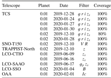
Table 1. Observing log of ground-based photometric observations.

Telescope Planet Date Filter Coverage

TCS 0.01 2019-12-28 g r i zs 100% 0.01 2020-01-24 g r i zs 100% 0.01 2020-01-27 g r i zs 100% 0.01 2020-01-30 g r i zs 100% 0.02 2019-12-10 g r i zs 80% 0.02 2020-01-28 g r i zs 100% SNO-T150 0.02 2019-12-10 V R 100% TRAPPIST-North 0.02 2019-12-10 z 100% LCO-CTIO 0.01 2019-06-09 zs 100% 0.01 2019-06-16 zs 100% LCO-SAAO 0.01 2019-06-17 gpzs 100% LCO-SSO 0.02 2020-01-04 B 100% OAA 0.01 2020-02-01 Ic 100%

and in both cases the transit shape is not clear, so we cannot claim the presence of a third transiting planet in the system. The analysis of future TESS re-observations of this object should help solve this ambiguity.

3. Ground-based follow-up observations

3.1. Seeing-limited transit photometry

We acquired ground-based time-series follow-up photometry of LTT 3780 as part of the TESS Follow-up Observing Program (TFOP)4 _{to attempt to (i) rule out nearby eclipsing binaries as} potential sources of the TESS detection, (ii) detect the transit-like event on target to confirm the event depth and thus the TESS photometric deblending factor, (iii) refine the TESS ephemeris, (iv) provide additional epochs of transit centre time measure-ments to supplement the transit timing variation analysis, and (v) place constraints on transit depth differences across optical filter bands. We used the TESS Transit Finder, which is a cus-tomised version of the Tapir software package (Jensen 2013), to schedule our transit observations. Unless otherwise noted, the photometric data were extracted using the AstroImageJ software package (Collins et al. 2017). A summary of the photometric ground-based observations is shown in Table15_. 3.1.1. Las Cumbres Observatory network

In total, four transits of the LTT 3780 system where observed with the SINISTRO CCDs operating in the 1m telescopes of the Las Cumbres Observatory (LCOGT) network6_{(Brown et al.} 2013). For LTT 3780 b, two transits were observed from the Cerro Tololo Inter-American Observatory (CTIO) site using the zsfilter on 9 and 16 June 2019. Exposure times were set to 45 and

70 s, respectively, and an optimum aperture of 15.0 pix (5.8300_).

A third transit was observed using the gp and zsfilters from the

South Africa Astronomical Observatory (SAAO) site on 17 June 2019 with exposure times of 140 s and the optimum apertures of 12.0 pix (4.6700_{) and 15.0 pix (5.83}00_{) for filters gpand zs,}

respec-tively. For LTT 3780 c, one transit observation was performed from Siding Spring Observatory (SSO) on 4 January 2020, using

4 _{https://tess.mit.edu/followup/}

5 _{The LCOGT, TRAPPIST-North, SNO-T150, OAA, and MuSCAT2}

light curves can be provided upon request to the first author.

the B filter, an exposure time of 140 s and an optimum aperture of 7 pix (2.6600_).

3.1.2. TRAPPIST-North

TRAPPIST-North at Oukaimeden Observatory in Morocco is a 60 cm Ritchey-Chrétien telescope, which has a thermo-electrically cooled 2k × 2k Andor iKon-L BEX2DD CCD cam-era with a field of view of 200_{× 20}0_{and pixel scale of 0.60}00_pix−1

(Jehin et al. 2011; Barkaoui et al. 2019). We carried out a full-transit observation of TOI–732.02 on 10 December 2019 using a z filter with an exposure time of 10 s. We took 507 images and performed aperture photometry with an optimum aperture of 11 pixels (6.600_{) and a point spread function (PSF) full width}

half maximum (FWHM) of 3.700_{. We confirmed the event on}

the target star with a depth of ∼3.2 ppt (parts per thousand) and occurring about 1 h sooner with respect to the predicted ingress, but still within the expected uncertainty from an ephemeris derived from the TESS data only. We cleared all the stars of eclipsing binaries within the 2.50_{around the target star.}

3.1.3. Sierra Nevada Observatory-T150 multicolour photometry

T150 at Sierra Nevada Observatory (SNO) in Granada (Spain) is a 150 cm Ritchey-Chrétien telescope equipped with another thermo-electrically cooled 2k × 2k Andor iKon-L BEX2DD CCD camera with a field of view of 7.90_{× 7.9}0 _{and pixel scale}

of 0.2300_pix−1_{. We carried out a full-transit observation of TOI–}

732.02 on 10 December 2019 with R and V filters (placed on a filter wheel) with an exposure time of 20 and 60 s, respectively. We took 125 images (2 × 2 binning) in both filters, and per-formed aperture photometry with an optimum aperture of 10 pix (4.600_{) in R and 11 pix (5.0}00_{) in V and a PSF FWHM of 2.3}00

and 2.700_{, respectively. We confirmed the event on the target star}

in both filters, with similar depth of ∼3.2 ppt and also about 1 h earlier than the predicted ingress.

3.1.4. Observatori Astronòmic Albanyà

Additional photometric observations of TOI–732.01 were acquired on 1 February 2020 with the 0.4 m telescope at the Observatori Astronòmic Albanyà (OAA), in Catalonia, Spain. The host star was observed for 391.7 min with a Cousins Ic

fil-ter and a Moravian G4-9000 camera with a field of view of 3056(H) × 3056(V) pixels covering 36.80_{. We performed}

aper-ture photometry with an optimum aperaper-ture of 14 pix (20.300_{) and}

a PSF FWHM of 13.000_{. We confirmed the event on the target}

with depth of ∼2.9 ppt and occurring about 15 min later than the predicted ingress (within the expected uncertainty of the ephemeris derived from the TESS data only).

3.1.5. Telescopio Carlos Sánchez/MuSCAT2 multicolour photometry

We observed four transits of TOI–732.01 and two transits of TOI–732.02 with the MuSCAT2 multi-colour imager (Narita et al. 2019) installed at the Telescopio Carlos Sánchez (TCS), located at the Teide Observatory in Tenerife, Spain. The instru-ment carries out high-precision, simultaneous photometry in four colours (g, r, i, zs) with a pixel scale of 0.4400pix−1.

Obser-vations were reduced with a dedicated MuSCAT2 pipeline (see

Parviainen et al. 2019, for details).

The exposure times varied from passband to passband and night to night depending on observing conditions and the observer’s judgement. The shortest exposure times were of the order of 5 s, and the longest of 60 s. The aperture photometry was performed with an the optimum apertures of 5–600_,

depend-ing on the seedepend-ing and possible defocusdepend-ing at a given observdepend-ing night. The reduction included an initial detrending, after which all the light curves were down-sampled to a 1 min cadence. The covariates used in the detrending were also down-sampled and stored, and used in the linear baseline model in the final joint light curve and RV modelling.

3.2. Other light curves from public databases

We compiled photometric series obtained by long-time base-line automated surveys as inDíez Alonso et al.(2019). We were only able to retrieve data from the All-Sky Automated Survey for Supernovae (ASAS-SN;Kochanek et al. 2017), but not from other public catalogues, such as the All-Sky Automated Sur-vey (ASAS;Pojmanski 2002), Northern Sky Variability Survey (NSVS;Wo´zniak et al. 2004), The MEarth Project (Charbonneau et al. 2008), the Catalina surveys (Drake et al. 2014), or the Hun-garian Automated Telescope Network (Bakos et al. 2004). The ASAS-SN dataset comprises 220 observations spanning about 2000 d in V band.

Additionally, LTT 3780 is a candidate of the Super-Wide Angle Search for Planets (SuperWASP; Pollacco et al. 2006). SuperWASP acquired more than 40 000 photometric observa-tions using a broad-band optical filter spanning two consecutive seasons from January to June 2013, and January to June 2014. For our search to detect long-term photometric modulations associated with the stellar rotation, we binned the data to one-day intervals, resulting in 191 epochs.

3.3. High-contrast imaging

The presence of an unknown star within the same TESS pixel as the target can result in under-estimated planetary radii, caused by the additional light diluting the transit depth. These unac-counted stars could also potentially be the source of astrophysical false positives, although this was found to be unlikely for multi-planet transiting systems (Lissauer et al. 2012). To search for close-in companion stars (bound or unbound to the target star), and to estimate the potential contamination factor from such sources, we used high-contrast images of LTT 3780 acquired with four instruments: (1) FastCam (Oscoz et al. 2008) mounted on the 1.5 m TCS (see Sect. 3.1.5); (2) HRCam (Tokovinin 2018) installed on the 4.1 m Southern Astrophysical Research (SOAR) telescope at CTIO; (3) ‘Alopeke7_{, a high-resolution} speckle interferometry instrument on the 8 m Frederick C. Gillett Gemini North telescope at Gemini North Observatory, Hawai’i, USA; and (4) Near InfraRed Imager and spectrograph (NIRI,

Hodapp et al. 2003) coupled with the adaptive optics (AO) system facility, ALTAIR, mounted also on Gemini North. 3.3.1. TCS/FastCam lucky imaging

LTT 3780 was observed with the FastCam instrument on 22 May 2014 in the I band as part of our high-resolution imaging campaign to identify and characterise the binary content of the CARMENES sample of M dwarfs (Cortés-Contreras et al. 2017).

7 _{https://www.gemini.edu/sciops/instruments/} alopeke-zorro/

−5 0 5 X (arcsec) −4 −2 0 2 4 Y (a rcsec) (a) TCS/FastCam −1 0 1 X (arcsec) −1 0 1 (b) SOAR/HRCam −2 0 2 X (arcsec) −2 −1 0 1 2(c) Gemini-N/ALTAIR+NIRI −1 0 1 X (arcsec) −1.0 −0.5 0.0 0.5 1.0 (d) Gemini-N/Alopeke

Fig. 3.High-spatial-resolution images of LTT 3780 from TCS/FastCam lucky imaging (panel a), SOAR/HRCam speckle imaging (panel b), Gemini North/ALTAIR+NIRI (panel c), and Gemini North/‘Alopeke at 832 nm (panel d). The dotted circle corresponds to 100_{and the dashed circle to 3}00

separation. North is up and east is left.

0.1 1

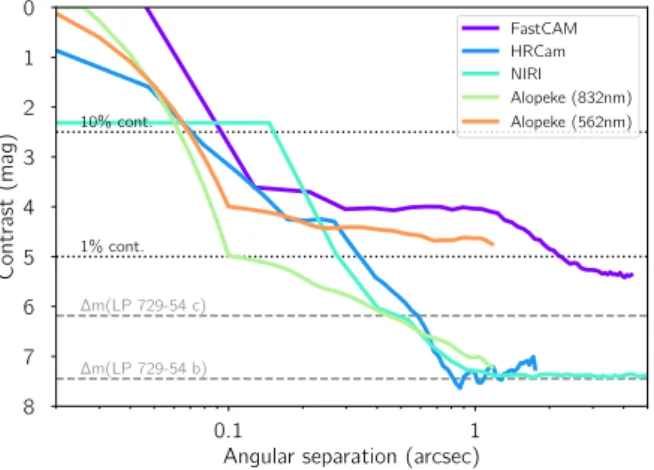
Angular separation (arcsec) 0 1 2 3 4 5 6 7 8 Contrast (mag) 10% cont. 1% cont. ∆m(LP 729-54 b) ∆m(LP 729-54 c) FastCAM HRCam NIRI Alopeke (832nm) Alopeke (562nm)

Fig. 4. Sensitivity curves (5σ limits) for all five high-spatial resolu-tion images used in this work. The 1 and 10% contaminaresolu-tion levels are marked as black dotted horizontal lines and the maximum magnitude contrast that a blended binary could have to mimic the transit depth of the two planets in the system are marked as grey dashed horizontal lines. FastCam is a lucky imaging camera mounted on TCS and is equipped with a high readout speed and sub-electron noise L3CCD Andor 512 × 512 detector, with a pixel size of 0.042500_,

which provides a field of view of 21.200_{× 21.2}00_{. Ten blocks of}

1000 individual frames of 50 ms exposure time were obtained for this target. Data were processed using a dedicated pipeline developed by the Universidad Politécnica de Cartagena group (seeLabadie et al. 2010;Jódar et al. 2013), which includes bias correction, the alignment and combination of images, and the selection of the best-quality images using the pixel position and value of the brightest speckle. Figure 3a shows the FastCam image resulting from selecting the 50% best-quality images of the first 4000 frames. The corresponding 5σ detection sensitiv-ity curve is shown in Fig. 4. No additional source is detected with δ I < 4 mag down to the resolution limit of the telescope (∼0.1500_).

3.3.2. SOAR/HRCam speckle imaging

LTT 3780 was observed with SOAR/HRCam speckle imaging on 12 December 2019 (UT) in I band, a similar visible band-pass to that of TESS, to search for nearby sources. Further details of observations are available in Ziegler et al. (2020). The region within 300 _{of LTT 3780 was found to be devoid of}

nearby stars (see Fig.3b) within the 5σ detection sensitivity of the observation, which is shown in Fig.4.

3.3.3. Gemini North/‘Alopeke speckle imaging

LTT 3780 was observed on 17 February 2020 (UT) at Gemini North with ‘Alopeke, the high-resolution speckle interferome-try instrument. The star was observed simultaneously in two bandpasses centred at 562 nm and 832 nm (the latter is shown in Fig.3d). The resulting contrast curves are shown in Fig.4, from which we deduced that LTT 3780 does not have any close com-panion. At the distance of LTT 3780, our inner working angle is 0.37 au at 562 nm and 0.62 au at 832 nm, respectively, and our field of view (r = 1.2500_{) extends out to 28 au from the star. Given}

that LTT 3780 is an M3.5 V star, our contrast curves eliminate any companion object down to the M–L boundary in luminosity. 3.3.4. Gemini-North/NIRI+ALTAIR AO imaging

On 25 November 2019 (UT) we acquired AO images of LTT 3780 with the Gemini North/NIRI+ALTAIR using the Brγ filter (Gemini-North ID G0218) centred at 2.17 µm. We collected nine images, each with an integration time of 2.2 s, and dithered the telescope between each exposure. Images were reduced fol-lowing standard procedures, that is, correction for bad pixels, flat-fielding, subtraction of a sky background constructed from the dithered images, alignment of the star between frames, and co-addition of data. The Gemini North/NIRI+ALTAIR AO image of LTT 3780 (see Fig.3c) revealed no close-in compan-ions and the star appeared single to the limit of our resolution. Figure4presents the 5σ contrast curve as a function of the angu-lar separation from LTT 3780. We calculated the sensitivity to faint companions as a function of radius by injecting synthetic point spread functions at a range of magnitudes into the data, and measuring the significance at which they could be recovered. The data were of high quality, and we were sensitive to compan-ions 5.0 mag fainter than the target at just 270 mas, and 7.4 mag fainter than the target at separations greater than ∼100_.

3.4. High-resolution spectroscopy 3.4.1. 3.5 m Calar Alto/CARMENES

We obtained 52 high-resolution spectra of LTT 3780 between 27 December 2019 (UT) and 19 February 2020 (UT) with the CARMENES instrument (Quirrenbach et al. 2014, 2018) mounted on the 3.5 m telescope at the Calar Alto Observa-tory, Almería, Spain, as part of the guaranteed time observation program to search for exoplanets around M dwarfs (Reiners et al. 2018). The CARMENES spectrograph has two channels, the visible (VIS) one covering the spectral range 0.52–0.96 µm

and a near-infrared (NIR) channel covering the spectral range 0.96–1.71 µm.

Relative radial-velocity values, chromatic index (CRX), dif-ferential line width (dLW), and Hα index values were obtained using serval8 _{(Zechmeister et al. 2018). For each spectrum,} we also computed the cross-correlation function (CCF) and its FWHM, contrast (CTR) and bisector velocity span (BVS) values, followingLafarga et al.(2020). The RV measurements were cor-rected for barycentric motion, secular acceleration, and nightly zero-points. For more details, see Trifonov et al. (2018) and

Kaminski et al.(2018). 3.4.2. Subaru/IRD

We observed LTT 3780 with the InfraRed Doppler instrument (IRD,Kotani et al. 2018) behind an AO system (AO188,Hayano et al. 2010) on the Subaru 8.2 m telescope on Mauna Kea Obser-vatories, as part of the Subaru IRD-TESS intensive follow-up project (S19A–069I). We took four spectra of LTT 3780 on 10 December 2019 (UT) and one spectrum on 13 December 2019 simultaneously with laser-frequency comb spectra. Expo-sure times were 480 s and a S/N at 1.0 µm was ∼100 for the four spectra, but the S/N was only ∼15 for the last one owing to thick clouds. We reduced the raw IRD frames of LTT 3780 using the echelle package of iraf for flat-fielding, scattered-light subtraction, aperture tracing, and wavelength calibration with the Th-Ar lamp spectra. For RV measurements requiring a more precise wavelength calibration, the wavelength was re-calibrated based on the emission lines of the combined laser frequency comb, which was injected simultaneously into both stellar and reference fibres during instrument calibrations. We injected these reduced spectra into the RV analysis pipeline for Subaru/IRD (Hirano et al. 2020) and attempted to reproduce the intrinsic stellar template spectrum from all the observed spec-tra with instrumental profile deconvolution and telluric removal. Radial velocities were measured with respect to that template by forward-modelling of the observed individual spectral segments (each spanning 0.7–1.0 nm). We found that the RV precision for the first-night spectra was typically 2.4 m s−1_{, while that of the}

second night was ≈19 m s−1 _{due to the low quality of the}

spec-trum. We therefore discarded the latter measurement from the final analysis.

3.4.3. NASA Infrared Telescope Facility/iSHELL

We obtained 77 five-minute spectra during seven nights for LP 729-54 spanning 28 days from January to February 2020 with the iSHELL spectrometer on the NASA Infrared Telescope Facility (IRTF,Rayner et al. 2016). Five-minute exposures were repeated 8–15 times within a night to reach a cumulative photon S/N per spectral pixel at about 2.2 µm (at the approximate cen-tre of the blaze for the middle order) varying from 152 to 205 to achieve a per-night RV precision of 6–10 m s−1_{. Spectra were}

reduced and RVs extracted using the methods outlined inCale et al.(2019).

Due to the limited barycentre sampling of the iSHELL obser-vations over the small observing window, the underlying stellar spectrum could not be well-isolated from other spectral features (namely tellurics). Therefore, a synthetic stellar spectrum was used to compute the RVs instead of deriving a more robust stel-lar template from the observations themselves. The overall RV scatter is consequently larger than expected given the S/N and

8 _{https://github.com/mzechmeister/serval}

RV information content of the observations. Two outliers (first and fourth night) were disregarded in the analysis, which can be recovered in the future with additional observations at different barycentre velocities.

The radial velocities collected with 3.5 m Calar Alto/ CARMENES, Subaru/IRD and IRTF/iSHELL instruments and their uncertainties are listed in TableA.1.

4. Stellar parameters

4.1. The stellar host and its binary system

LTT 3780 is a relatively bright (J ≈ 9.0 mag) M3.5 V star at approximately 22 pc (Gaia Collaboration 2018). According to the Washington Double Star catalogue (Mason et al. 2001), it is the primary of the poorly investigated wide system LDS 3977 (Luyten 1963). The secondary, located at angular separation ρ_{= 15.81 ± 0.15}00_{and position angle θ = 96.9 ± 0.2 deg (at epoch} J2015.5), is LP 729–55, which is about 2.1 mag fainter in the J band and shares within 1σ the same parallax and proper motions as LTT 3780 (Gaia Collaboration 2018). At the system heliocentric distance, ρ translates into a projected physical sepa-ration of s = 348 ± 3 au.Reid et al.(2003) assigned the spectral type M3.5 V to the secondary from low-resolution spectroscopy. However, we consider that they meant the primary instead, whose spectral type agrees within 0.5 dex with that derived by Scholz et al. (2005), as well as with its effective tempera-ture (see below). From accurate absolute magnitudes, colours, and luminosity and using various magnitude-, colour-, and luminosity-spectral type relationships available in the literature for solar-metallicity M-type stars, we estimate an m5.0 ± 0.5 V spectral type for the common proper companion secondary LP 729–55.

4.2. Photospheric and physical parameters

The photospheric parameters of LTT 3780 were determined fol-lowingPassegger et al.(2019) using improved PHOENIX-ACES (Husser et al. 2013) stellar atmosphere models, which include a new equation of state to especially account for spectral features of low-temperature stellar atmospheres, as well as new atomic and molecular line lists. Effective temperature, surface grav-ity, and metallicity were derived assuming v sin i? = 2 km s−1

and a stellar age of 5 Gyr (see Passegger et al. 2019). The lat-ter two values are consistent with the rotational velocity upper limit determined by Jeffers et al. (2018) and an approximate solar age from the kinematic membership in the Galactic thin disc, using the same Galactocentric space velocity computation asCortés-Contreras(2016).

To compute the physical parameters we followed the multi-step approach ofSchweitzer et al.(2019). First, we determined the luminosity L by integrating the photometric stellar energy distribution collected for the CARMENES targets (Caballero et al. 2016) with the Virtual Observatory Spectral energy dis-tribution Analyser (Bayo et al. 2008) using parallactic distances from the Gaia DR2 catalogue (Gaia Collaboration 2018). We then derived the radius R and mass M using the Stefan-Boltzmann’s law and the empirical M-R relation presented in

Schweitzer et al.(2019), respectively.

We derived an effective temperature of Teff =3360 ± 51 K, a

stellar mass of M? =0.379 ± 0.016 M, and a radius of R? =

0.382 ± 0.012 R, resulting in a stellar density of ρ = 9.6 ±

1.0 g cm−3_{. All derived values and additional stellar parameters}

Table 2. Stellar parameters of LTT 3780.

Parameter Value Reference

Name and identifiers

Name LTT 3470 Luyten(1957)

G 162–44 Giclas et al.(1971)

Karmn J10185–117 Caballero et al.(2016)

TOI 732 TESS Alerts

TIC 36 724 087 Stassun et al.(2018)

Coordinates and spectral type

α(J2015.5) 10:18:34.77 Gaia DR2

δ(J2015.5) –11:43:04.1 Gaia DR2

Sp. type M3.5 V Reid et al.(2003)

Magnitudes B (mag) 14.68 ± 0.04 UCAC4 g(mag) 13.84 ± 0.05 UCAC4 GBP(mag) 13.352 ± 0.004 Gaia DR2 V (mag) 13.14 ± 0.04 UCAC4 r (mag) 12.55 ± 0.05 UCAC4 G (mag) 11.8465 ± 0.0005 Gaia DR2 i (mag) 11.09 ± 0.08 UCAC4 GRP(mag) 10.6583 ± 0.0016 Gaia DR2 J (mag) 9.01 ± 0.03 2MASS H (mag) 8.44 ± 0.06 2MASS Ks(mag) 8.20 ± 0.02 2MASS W1 (mag) 8.04 ± 0.02 AllWISE W2 (mag) 7.880 ± 0.019 AllWISE W3 (mag) 7.771 ± 0.019 AllWISE W4 (mag) 7.58 ± 0.17 AllWISE

Parallax and kinematics

π(mas) 45.46 ± 0.08 Gaia DR2

d (pc) 22.00 ± 0.04 Gaia DR2

µαcos δ (mas yr−1) −341.411 ± 0.11 Gaia DR2

µδ(mas yr−1) −247.87 ± 0.10 Gaia DR2

Vr(km s−1) −0.44 ± 0.09 Jeffers et al.(2018)

U (km s−1_{) −14.89 ± 0.06 This work}

V (km s−1_{) −22.00 ± 0.08 This work}

W (km s−1_{) −35.08 ± 0.07 This work}

Galactic population Thin disc This work

Photospheric parameters

Teff(K) 3360 ± 51 This work

log g 4.81 ± 0.04 This work

[Fe/H] +0.09 ± 0.16 This work

vsin i?(km s−1) <3.0 Jeffers et al.(2018)

Physical parameters

L (10−4_{L) 167 ± 3 This work}

R (R) 0.382 ± 0.012 This work

M (M) 0.379 ± 0.016 This work

ρ(g cm−3) 9.6 ± 1.0 This work

References. 2MASS:Skrutskie et al.(2006); AllWISE:Cutri & et al.

(2013); Gaia DR2:Gaia Collaboration(2018); UCAC4:Zacharias et al.

(2013).

4.3. Stellar activity and rotation period

Using the stellar radius determined in Sect.4.2 and presented in Table 2 (R?= 0.382 ± 0.012 R) and the upper limit for

the stellar projected rotation velocity found by Jeffers et al.

(2018, vrotsin i?< 3 km s−1), we calculated the stellar rotation

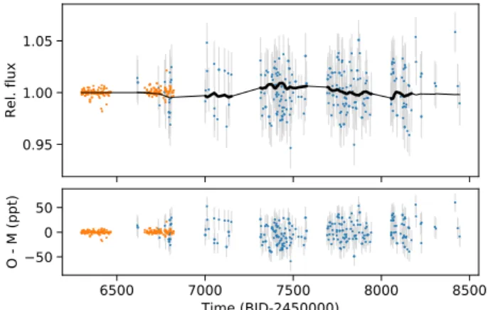
0.95 1.00 1.05 Rel. flux 6500 7000 7500 8000 8500 Time (BJD-2450000) 500 50 O - M (ppt)

Fig. 5.SuperWASP (orange) and ASAS-SN (blue) long-term photomet-ric monitoring modelled with a quasi-periodic GP kernel defined as in

Foreman-Mackey et al.(2017).

period Prot to be longer than 6 d, and shorter than 100 d for

vrotsin i?> 0.2 km s−1. We performed a search for the rotation

period in the existing photometric data of LTT 3780 from the SuperWASP and ASAS-SN surveys. The ASAS-SN photome-try shows no variation at the precision of the data. However, an analysis using a quasi-periodic Gaussian process (GP) suggested a 66 ± 2 d period signal in the data (see Fig.5), albeit not with very high significance. We used the quasi-periodic GP kernel introduced byForeman-Mackey et al.(2017) of the form ki, j(τ) = B 2 + Ce−τ/L " cos 2πτ Prot ! +(1 + C) # ,

where τ = |ti− tj| is the time-lag, B and C define the amplitude of

the GP, L is a timescale for the amplitude modulation of the GP, and Protis the period of the quasi-periodic modulations. For the

fit, we considered that each instrument and pass band could have different values of B and C, while L and Protwere left as

com-mon parameters. We considered wide uninformative priors for B, C (log-uniform between 10−3_{and 10}6_{), L (log-uniform between}

100_{d and 10}8_{d), P}

rot(uniform between 10 and 100 d), and

instru-mental jitter (log-uniform between 10 ppm and 106_{ppm). The 3σ}

upper limit implied by this latter fit is 300 ppm, which demon-strates that LTT 3780 is magnetically inactive with only very few starspots. The photometric variability can be explained by a small starspot or group of starspots not exceeding approximately 2% of the total area of the star assuming a star-spot temperature difference of 500 K. This is in agreement with the estimate of the RV amplitude that one could expect from rotational modu-lation following the prescription given byAigrain et al.(2012). Additionally, the Hα activity indicator shows that LTT 3780 is an inactive star (Jeffers et al. 2018). Therefore, we conclude that the imprint of stellar activity signals in the collected CARMENES RVs is probably at the level of the measurement errors.

5. Analysis and results

5.1. Frequency analysis of radial velocities

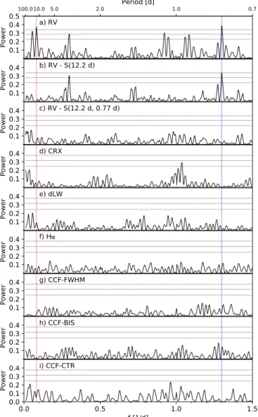
In order to search for the Doppler reflex motion induced by the transiting planets and unveil the presence of possible addi-tional signals in our time-series RV data, we performed a frequency analysis of the RV measurements and their activity indicators. We calculated the generalised Lomb-Scargle (GLS) periodograms (Zechmeister & Kürster 2009) of the available

0.1 0.2 0.3 0.4 0.5 Power a) RV 0.1 0.2 0.3 0.4 Power b) RV - S(12.2 d) 0.1 0.2 0.3 0.4 Power c) RV - S(12.2 d, 0.77 d) 0.1 0.2 0.3 0.4 Power d) CRX 0.1 0.2 0.3 0.4 Power e) dLW 0.1 0.2 0.3 0.4 Power f) H 0.1 0.2 0.3 0.4 Power g) CCF-FWHM 0.1 0.2 0.3 0.4 Power h) CCF-BIS 0.0 0.5 1.0 1.5 f [1/d] 0.0 0.1 0.2 0.3 0.4 Power i) CCF-CTR 100.010.0 5.0 2.0 Period [d] 1.0 0.7

Fig. 6.Generalised Lomb-Scargle periodograms for RVs of LTT 3780 (a), their residuals (b) after fitting a sinusoid with period and phase cor-responding to the transiting planet TOI-732.02 ( fc=0.081 ± 0.002 d−1,

Pc=12.3 ± 0.3 d), marked in red, and their residuals (c) after fitting

two sinusoids with periods and phases corresponding to the transit-ing planets TOI-732.02 and TOI-732.01 ( fb =1.298 ± 0.002 d−1, Pb=

0.770 ± 0.001 d), marked in blue. Panels d–i: periodograms of the chro-matic index, differential line width, Hα index, cross-correlation function FWHM, bisector velocity span, and contrast, all of them derived only from CARMENES observations. Horizontal lines show the theoretical FAP levels of 10% (short-dashed line), 1% (long-dashed line), and 0.1% (dot-dashed line) for each panel.

time series and computed the theoretical 10, 1, and 0.1% false alarm probability (FAP) levels (Fig.6). The 70 d time baseline of the RV measurements translates into a frequency resolution of 0.01428 d−1_.

The GLS periodogram of the CARMENES data (Fig. 6a) shows two highly significant peaks (FAP < 0.1%) at the orbital frequencies of the transiting planets, TOI–732.02 ( fc=0.081 ±

0.002 d−1_{, Pc = 12.3 ± 0.3 d) and TOI–732.01 ( fb = 1.298 ±}

0.002 d−1_{, Pb=0.770 ± 0.001 d). The RV residuals after a joint}

fit with two circular orbits, fixed periods, and transit mid-times given by the TESS ephemerides showed no further significant peaks (Fig.6c).

We also calculated periodograms for different activity indi-cators computed by SERVAL, namely the CRX (Fig.6d), dLW

(Fig. 6e), and Hα index (Fig. 6f), and some indicators from the cross-correlation function such as FWHM, BIS, and CTR (Figs. 6g–i). No significant peaks were found except for some power with periods close to 1 d in CRX, which are related to the sampling of the observations. There are no peaks in any activity indicator at the frequency of the transiting planets.

5.2. Joint modelling of the light curves and RVs

We modelled the TESS light curve, the ground-based light curves, and the RVs simultaneously using PyTransit (Parviainen 2015). The analysis followed the approach described in Parviainen et al. (2019, 2020), namely we estimated any possible flux contamination from unresolved sources inside the photometry apertures in the TESS and ground-based photometry together with the planetary parameters.

The TESS dataset included in the analysis consisted of 2.4 h windows of SAP light curves produced by the SPOC pipeline (Twicken et al. 2010; Jenkins et al. 2016; Morris et al. 2017) centred around each individual transit centre normalised to the median per-window out-of-transit flux. The SAP light curves were chosen over the PDC light curves because the trends in the light curve are dominated by the photon noise (on 2.4 h time scales), and because the PDC process removes the PDC-estimated flux contamination. The latter can introduce biases into our contamination estimation if the PDC contamination is overestimated, as we did not allow for negative contamination. By chance, the TESS dataset did not contain transits with overlapping windows. The ground-based photometry dataset included all the ground-based transit observations described in Sect.3. We binned the MuSCAT2 photometry to a time cadence of one minute, but did not otherwise modify the data. The RV dataset was taken as it was, and included the 3.5 m Calar Alto/CARMENES and Subaru/IRD usable RVs described in Sect.3.4.

5.2.1. Parametrisation

The joint model contained 207 free parameters, but most of them were linear coefficients used to model systematic trends in the ground-based light curves, and not of scientific interest. Of these 207 parameters, we used only 31 for describing the planets and their orbits, stellar limb darkening, and flux contamination.

Planet. Each planet and its orbit were parametrised by the orbital period, zero epoch, true planet-star area ratio, impact parameter, two parameters describing the eccentricity and argu-ment of periastron, and RV semi-amplitude, as detailed in Table B.1. Here we made a distinction between the apparent and true planet-star area ratios. The apparent area ratio can be affected by flux contamination that leads to passband- and aperture-size-dependent variations in the apparent transit depth. However, the true area ratio stands for the uncontaminated geo-metric planet-star area ratio and, unlike the apparent area ratio, is independent of passband and photometry aperture size. In addi-tion to these per-planet parameters, the stellar density was used to complete the description of the orbit.

Limb darkening. We parametrised the stellar limb darken-ing with the triangular parametrisation for the quadratic limb darkening model introduced byKipping(2013), and constrained it using the code LDTk (Parviainen & Aigrain 2015). This yielded two parameters per passband, totalling 12 parameters for the six passbands for which we have photometric data.

Contamination. The TESS photometry was given an unconstrained contamination factor independent of the contam-ination for the ground-based observations, while the contami-nation in the ground-based observations was modelled using a physical model introduced by Parviainen et al. (2019). This is because the TESS pixel size is significantly larger than the pixel size of the ground-based instruments used for the study, and thus we expected the contamination in the TESS data to be larger than in the ground-based photometry. In brief, the observed flux (Fapp), which can be used to determine the apparent planet-star

radius ratio (kapp) by fitting the transit model, in the light

con-tamination model of Parviainen et al. (2019) is defined as a linear combination of the host and contaminant star fluxes (pos-sibly from several contaminating sources). The contamination (c) is calculated for a set of passbands (i) given the passband transmission functions (T ), the effective temperatures of host (Teff,H), and contaminant stars (Teff,C), necessary to calculate

rel-ative fluxes of host (FH) and contaminant star (FC), and the level

of contamination in some reference passband (c0):

ci= FC,i

FH,i+FC,i.

By combining a contamination model with a transit model and taking into account that the transit depth scales linearly with the contamination factor, the true, uncontaminated radius ratio of a transiting planet (ktrue) can be calculated as:

ktrue=kapp/√1 − c.

Trends and noise. We chose to use a simple linear model to explain the trends in the photometry. That is, the photome-try (sans transit) was explained as a dot product of a baseline coefficient vector and a covariate vector. The ground-based light curves were observed with different instruments and the pho-tometry was reduced with different phopho-tometry pipelines. Thus, the exact set of covariates included in the baseline model varied from light curve to light curve, but the airmass, x- and y-centroid shifts, and PSF FWHM were included whenever possible. The TESS photometry was given a constant baseline fixed to unity, because adding a per-transit model would increase the number of model parameters excessively.

We also chose to use a linear baseline model rather than to model the systematics as a GP because the latter approach would have added a significant layer of complexity to the analysis of such a heterogeneous dataset. Using a GP would require a sepa-rate kernel for each light curve source (since we have varying sets of covariates available), and the computation time would increase significantly.

5.2.2. Joint modelling results

The analysis was carried out for two cases: (a) unconstrained contamination in the ground-based light curves, and (b) assum-ing no contamination in the ground-based light curves. The contamination in the TESS photometry was unconstrained in both cases, and independent of the ground-based contamination. The first case, (a) was used to determine whether or not the ground-based photometry contained additional flux from any unresolved source. The analysis excluded significant con-tamination from any source of different spectral type than the host star in the ground-based observations (i.e. only passband-independent contamination was allowed, which would require the contaminating source to have the same spectral type as the host star).

Since all the additional observational data rule out an almost identical nearby star, we assumed that the ground-based photom-etry did not contain significant contamination, in agreement with the results of the ground-based follow-up presented in Sect.3. Therefore, we chose the parameter posteriors from the second case as our final parameter estimates, and present them here. The parameter estimates for the first case are available from GitHub with the rest of the analyses.

Finally, we report the model posterior parameter estimates in Table 3. The posterior model is shown in Figs. 7 and 8, and parameter posteriors are shown for selected parameters in Figs.B.1andB.2.

6. Discussion

6.1. LTT 3780 b and c: two planets in the same system straddling the radius gap

The LTT 3780 system consists of two small transiting plan-ets. The ultra-short-period planet LTT 3780 b (Pb≈ 0.77 d) has

a radius of Rb= 1.35+_−0.060.06R⊕ and a mass of Mb= 2.34+_−0.230.24M⊕,

yielding a mean density of ρb= 5.24+_−0.810.94g cm−3. The outer

planet LTT 3780 c (Pc≈ 12.25 d) has a radius of Rc= 2.42+0.10_−0.10R⊕

and a mass of Mc= 6.29+0.63_−0.61M⊕, yielding a mean density of

ρc= 2.45+_−0.370.44g cm−3. This is the first planetary system around an

M dwarf with two planets located on opposite sides of the radius gap (Fulton et al. 2017;Fulton & Petigura 2018) that separates super-Earths from sub-Neptunes.

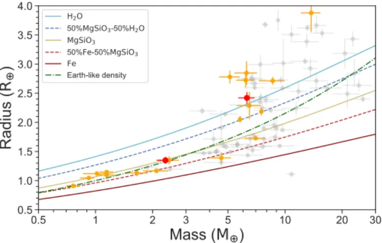
The positions of LTT 3780 b and LTT 3780 c on the mass-radius diagram are shown in Fig.9in comparison to the sample of small transiting planets (Rp≤ 4 R⊕) whose masses and radii

have been derived with a precision better than 20%9_{. The bulk} densities of the two planets are significantly different, and their positions in the mass–radius diagram indicate substantially dif-ferent compositions. Planet LTT 3780 b is compatible with an Earth-like bulk composition, ranging from 50% silicate and 50% iron to 100% silicate. On the other hand, LTT 3780 c has a bulk density consistent with a volatile-dominated world.

The architecture of the LTT 3780 planetary system is con-sistent with those of other systems hosting two or more small, close-in planets located on opposite sides of the radius gap: Kepler-10 bc (Dumusque et al. 2014), K2-106 bc (Sinukoff et al. 2017;Guenther et al. 2017), HD 3167 bc (K2-96 bc;Christiansen et al. 2017; Gandolfi et al. 2017), GJ 9827 bcd (K2-135 bcd;

Niraula et al. 2017; Prieto-Arranz et al. 2018), K2-138 bcdef (Christiansen et al. 2018; Lopez et al. 2019), HD 15337 bc (TOI-402 bc;Gandolfi et al. 2019;Dumusque et al. 2019), and K2-36 bc (Damasso et al. 2019). In all these systems, the close-in planets have smaller radii and higher mean densities, consis-tent with a rocky terrestrial composition, and the outer planets have larger radii and lower mean densities, suggesting that they are composed of rocky cores surrounded by light, hydrogen-dominated or water envelopes (see Fig.10). This result agrees with current theoretical scenarios that explain the existence of the radius gap by atmospheric escape (Owen & Wu 2017;Jin & Mordasini 2018).

All previously-known stars with small planets located on opposite sides of the radius gap have warmer effective temper-atures and higher masses than LTT 3780. Except for GJ 982710_,

9 _{http://www.astro.keele.ac.uk/jkt/tepcat/}

10 _{GJ 9827 should have been named BD–02 5958, as the third and last}

Gliese/Gliese-Jahreiss catalogue counted only from GJ 1 to GJ 4388 (Gliese & Jahreiß 1991).

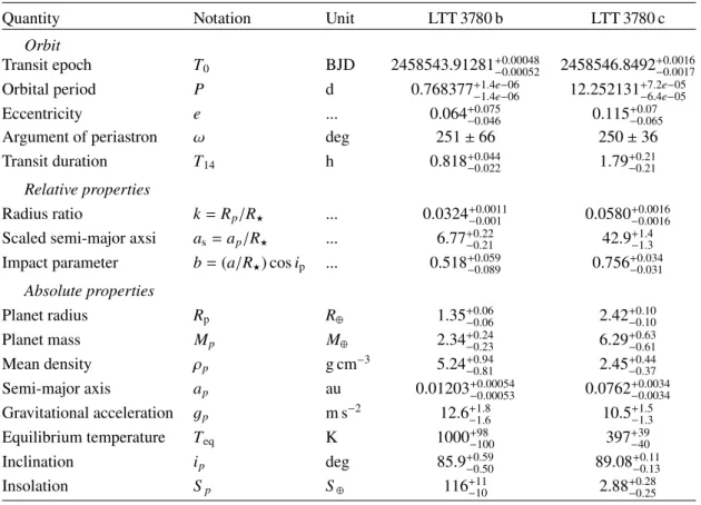
Table 3. Posterior estimates for the stellar and planetary parameters from the combined analysis.

Quantity Notation Unit LTT 3780 b LTT 3780 c

Orbit

Transit epoch T0 BJD 2458543.91281+_−0.000520.00048 2458546.8492+_−0.00170.0016

Orbital period P d 0.768377+_1.4e−06

−1.4e−06 12.252131+−6.4e−057.2e−05

Eccentricity e ... 0.064+0.075

−0.046 0.115+−0.0650.07

Argument of periastron ω deg 251 ± 66 250 ± 36

Transit duration T14 h 0.818+_−0.0220.044 1.79+_−0.210.21

Relative properties

Radius ratio k = Rp/R? ... 0.0324+_−0.0010.0011 0.0580+_−0.00160.0016

Scaled semi-major axsi as=ap/R? ... 6.77+_−0.210.22 42.9+_−1.31.4

Impact parameter b = (a/R?) cos ip ... 0.518+_−0.0890.059 0.756+_−0.0310.034

Absolute properties Planet radius Rp R⊕ 1.35+0.06_−0.06 2.42+0.10_−0.10 Planet mass Mp M⊕ 2.34+0.24_−0.23 6.29+0.63_−0.61 Mean density ρp g cm−3 5.24+0.94_−0.81 2.45+0.44_−0.37 Semi-major axis ap au 0.01203+0.00054_−0.00053 0.0762+0.0034_−0.0034 Gravitational acceleration gp m s−2 12.6+1.8_−1.6 10.5+1.5_−1.3 Equilibrium temperature Teq K 1000+₋₁₀₀98 397+₋₄₀39 Inclination ip deg 85.9+_−0.500.59 89.08+0.11_−0.13 Insolation Sp S⊕ 116+₋₁₀11 2.88+_−0.250.28

host stars effective temperatures and masses range between 4920 and 5810 K and 0.80 M and 0.93 M, respectively. The

previ-ous smallest and coolest such star host, GJ 9827, has Teff ≈

4260 K and M ≈ 0.66 M, consistent with its late K

spec-tral type (Joy & Abt 1974;Bidelman 1985;Stephenson 1986). However, LTT 3780 is significantly cooler (Teff ≈ 3360 K) and,

correspondingly, less massive (M ≈ 0.38 M).

6.2. The ultra-short period planet LTT 3780 b

With orbital period of Pb≈ 0.77 d, LTT 3780 b belongs to the

population of ultra-short period planets (USPs) and joins the relatively small group of transiting USPs with masses pre-cisely measured via radial velocities and, hence, determined bulk densities. Taking into account the density of LTT 3780 b (ρb= 5.24+0.94_−0.81g cm−3), this USP has probably undergone

sig-nificant evolution and lost its primary, hydrogen-dominated atmosphere. The low luminosity of LTT 3780, as expected from its late spectral type, is counterbalanced by the short semi-mayor axis of LTT 3780 b, which leads to a strong planetary insolation (Sb= 116+11₋₁₀S⊕).

The stellar properties of LTT 3780 and GJ 1151 (M4.5 V) are very similar (Passegger et al. 2018), both being relatively quiet stars. Although LTT 3780 is more distant from Earth and about half a magnitude fainter, it is worth searching for low-frequency radio emission from LTT 3780 possibly generated by the interaction of the star’s magnetospheric plasma with its USP, as suggested in the case of GJ 1151 (Vedantham et al. 2020). 6.3. System architecture

The architecture of the LTT 3780 system is analogous to that of Kepler-10, which has a (slightly larger and commensurately

more massive) rocky planet with an orbital period about 10% longer than that of LTT 3780 b (Batalha et al. 2011), and an outer planet with orbital period of 45 d, whose radius is within a few percent of that of LTT 3780 c (the mass of Kepler-10 c is poorly-constrained; Fressin et al. 2011; Weiss et al. 2016), and whose orbit is also inclined by ∼5–6 deg with respect to its inner ultra-short-period sibling. Multi-transiting planetary systems have few planets with orbital periods less than 1.6 d (Lissauer et al. 2014), and the high inclination of these two well-studied multi-planet systems with USPs (the inclinations of most other USP in Kepler multi-planet systems are not well constrained) supports the hypothesis that this paucity results at least in part from typical USPs being more highly inclined with respect to their planetary companions than the 1–2 deg value typ-ical for Kepler multi-planet systems found by Fabrycky et al.

(2014).

6.4. Atmospheric scenarios for LTT 3780 c

The estimated radii of LTT 3780 b and c provide a unique oppor-tunity to study the mechanisms that shape the Fulton gap (Fulton et al. 2017). While the proximity of LTT 3780 b to its host star and its relatively small radius suggest the challenging nature of maintaining an atmosphere on this planet, characterisation of the atmosphere of LTT 3780 c will shed light on the nature of the dominant atmospheric processes in action on this planet. While LTT 3780 c is not as appealing a target as TRAPPIST planets (TSM ∈ 20–45;Gillon et al. 2017;Grimm et al. 2018) or LHS 1140 b (TSM∼65;Dittmann et al. 2017), its transmission spectroscopy metric (TSM) defined byKempton et al.(2018) for JWST/NIRISS is ∼122, which is above the cutoff of TSM = 90 suggested for atmospheric characterisation of planets with radii 1.5 < Rp< 2.75 R⊕with JWST/NIRISS.

+2.458e6

10

5

0

5

10

RV [m/s]

LP 729 54 radial velocities

830

840

850

860

870

880

890

900

910

Time - 2458544 [BJD]

+2.458e6

5

0

5

O - M

10

5

0

5

10

RV [m/s]

LP 729 54 b (P = 0.7684 d)

0.3

0.2

0.1

0.0

0.1

0.2

0.3

Phase [d]

5

0

5

O - M

LP 729 54 c (P = 12.2521 d)

4

2

0

2

4

6

Phase [d]

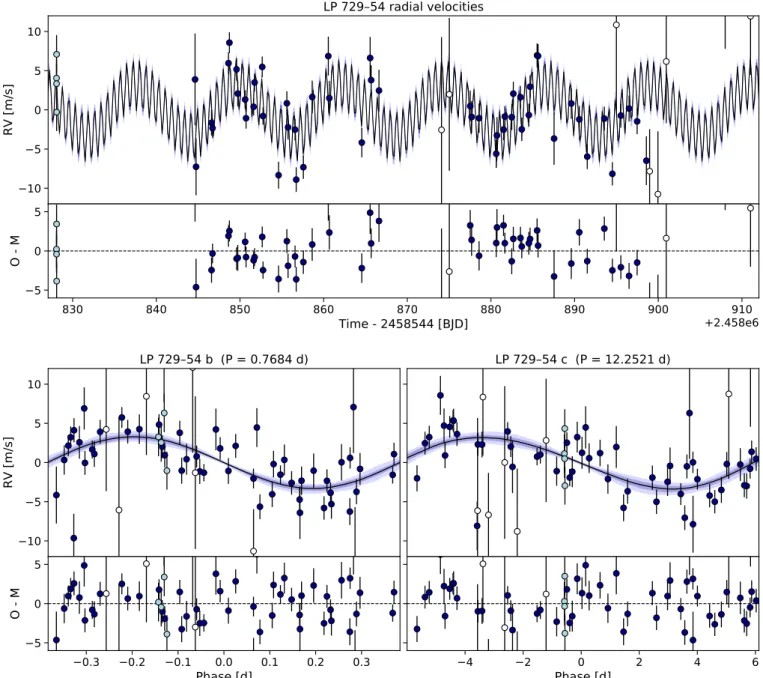
Fig. 7.Top panel: CARMENES (black circles), IRD (light blue circles), and iSHELL (open circles) RV measurements along with the residuals of the median posterior joint fit model (black line) and the 68, 95, and 99% central posterior limits (blue). Bottom panels: RVs phase-folded to the period of the two transiting planets (left: LTT 3780 b; right: LTT 3780 c).

In order to explore possible atmospheric scenar-ios of LTT 3780 c, we followed the approach outlined in

Molaverdikhani et al.(2019a), assuming that the planet sustains a substantial primary atmosphere. First we modelled the atmo-sphere self-consistently over a wide range of parameters using petitCODE(Mollière et al. 2015,2017). Given the uncertainties on the estimated equilibrium temperature of LTT 3780 c and possible missing feedback mechanisms in our self-consistent simulations, we chose the effective temperature as a free parameter with values of 350, 400, and 450 K (the equilibrium temperature derived for LTT 3780 c is 397+39

−40K). Since the

interior heat budget of exoplanets is not well understood, we assumed an interior heat budget contribution similar to that of Earth, i.e. ∼0.027 (e.g. Archer 2011). Slight deviations of the interior heat budget from this value do not change the results significantly. The atmospheric metallicity of planets seems to increase for less massive planets, both in the Solar System (e.g.

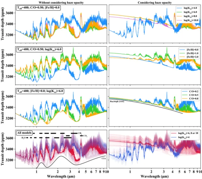
Molaverdikhani et al. 2019b) and beyond (Wakeford et al. 2017). Thus, we assumed three different metallicities, namely 1 ×, 10 ×, and 100 × solar metallicity, similar to those used byLuque et al. (2019). In addition, we also investigated the role of the carbon-to-oxygen ratio (C/O) in the atmosphere of LTT 3780 c, assuming C/O = 0.2 (sub-solar), 0.5 (∼solar), and 0.8 (super-solar). Altogether, 27 self-consistent temperature structures were calculated (Fig.11). No Earth-like cloud formation was included in our models.

In the next step we used these temperature structures as the input of our photochemical model (ChemKM;Molaverdikhani et al. 2019a,2020) to estimate abundances of atmospheric con-stituents. Studying the atmosphere of this planet required a validated chemical network over the assumed equilibrium tem-peratures. We therefore used theHébrard et al.(2012) full kinetic network (including 788 reactions and 135 H-C-O-N bearing species) and an updated version of their ultraviolet absorption

Fig. 8. Combined and phase-folded transits of LTT 3780 b and c for each passband. The blue points show the original photometry with the median baseline model removed, the black dots with error bars show the photometry binned to 10 min resolution, the black line shows the median posterior model, and the dark and light shaded areas show the 68 and 95% model posterior percentile limits, respectively.

cross-sections and branching yields. While the formation of hydrocarbon-based hazes is not fully understood (e.g. Hörst et al. 2018), it is believed that these processes start with the photolysis of haze precursor molecules such as CH4, C2H2,

HCN, and C6H6 (e.g. Molaverdikhani et al. 2020). The

cho-sen chemical network included all these precursor molecules and represented the haze particles collectively as one con-stituent called “soot” (e.g.Lavvas & Koskinen 2017). This soot included C8H6, C8H7, C10H3, C12H3, C12H10, C14H3, C2H4N, C2H3N2, C3H6N, C4H3N2, C4H8N, C5HN, C5H3N, C5H4N, 0.5 1 2 3 5 10 20 30

Mass (

M

)

R

ad

iu

s

(

R

)

Fig. 9. Mass-radius diagram for all planets with mass and radius measurement better than 20% (from the TEPCat9 _{database of} well-characterised planets; Southworth 2011). M-dwarf host planets are shown in orange, LTT 3780 b and LTT 3780 c with red dots. Theoreti-cal models (Zeng et al. 2016) are overplotted using different lines and colours. 1.5 2.0 2.5 3.0 3.5 Planet radius, Rp(R⊕) 0.0 2.5 5.0 7.5 10.0 12.5 Planet bulk density ,ρp (g/cm 3) Kepler-10 HD 15337 K2-138 LTT 3780 K2-36 GJ 9827 K2-106

Fig. 10.Radius–density diagram for multi-planet systems with planets on both sides of the radius gap. Different colours represent the different planetary systems, with the LTT 3780 planets marked and labelled in red. The vertical dotted line marks the centre of the radius gap at 1.7 R⊕.

C5H6N, C9H6N, C3H3O, C3H5O, C3H7O, and C4H6O, following

the convention outlined byHébrard et al.(2012).

The temperature of GJ 667C, another M-dwarf exoplanet host, is estimated to be around 3330 K (Neves et al. 2014), sim-ilar to that of LTT 3780. Consequently, we estimated the flux of LTT 3780 in the range of X-ray to optical wavelengths using GJ 667C data, obtained from the MUSCLES database (France et al. 2016). In addition to photolysis, we considered the effect of vertical mixing in the photochemical simulations by considering four values, 104_{, 10}6_{, 10}8_{, and 10}10_{cm s}−2_{, covering a wide range}

of possibilities from terrestrial values to tidally locked gaseous planets. In total, 108 photochemical models were calculated11_.

Examples of H2O, CH4, CO2, CO, and soot (haze particles)

abundances are shown in Fig. 11, assuming an effective tem-perature of 400 K, solar metallicity and solar C/O. In general, chemical depletion of H2O and CH4 are noticeable at strong

vertical mixing conditions, i.e. 106_{, 10}8 _{and 10}10_{cm s}−2_{, while}

CO2, CO, and soot particles show an enhancement in abundance

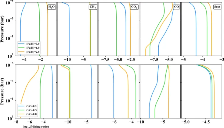
under such conditions. Figure12isolates the effect of metallicity

11 _{The atmospheric temperature structures, abundances and}

transmis-sion and emistransmis-sion spectra of these 108 models are publicly available at

250

500

750

10

10

10

10

Pressure (bar)

5

4

3

log10(Mixing ratio)

H2O log(Kzz)=4.0 log(Kzz)=6.0 log(Kzz)=8.0 log(K_zz)=10.0

20

10

30 20 10

30 20 10

20

10

Fig. 11. Left panel: simulated temperature structures of LTT 3780 c assuming a substantial primary atmosphere. Blue, green, and red curves represent the temperature profiles at different effective temperatures of 350, 400, and 450 K, respectively. Different profiles within each group are caused by different atmospheric metallicity and C/O ratio. There are 27 temperature structures in total. The dashed and solid black vertical lines mark 273.15 K (0◦_{C) and 373.15 K (100}◦_{C) for reference. Remaining panels: examples of atmospheric abundances of H2O, CH4, CO2, CO, and}

soot (haze particles), for solar metallicity and C/O ratio, and effective temperature of 400 K, resulting from the photo-chemical simulations at different vertical mixing strengths.

Fig. 12.Abundances of several atmospheric constituents at Teff=400 K. Top panels: solar C/O ratio, and Kzz= 106cm2s−1. Bottom panels: solar

metallicity and C/O ratios varying from 0.2 to 0.8.

(upper panels) and C/O ratio (lower panels) on the abundance of H2O, CH4, CO2, CO, and soot. For these illustrated examples,

we assumed an effective temperature of 400 K and a vertical mixing strength (Kzz) of 106cm2s−1. In general, increasing the

metallicity would enhance the production of most species at most altitudes under these conditions. However, given the highly non-linear nature of atmospheric feedback, some species could behave differently; see e.g. CO in the upper panel of Fig.12. The C/O ratio is modified by changing the oxygen elemental abun-dance and keeping the carbon elemental abunabun-dance the same. This represents a scenario in which gas or planetesimals accrete

onto a forming planet with different water content, while the car-bon content assumed to remain the same. Hence, variations of the C/O should not change methane abundances very much, as it has no oxygen compound. However, as a function of the depen-dency of the chemical formation pathway of a constituent on the formation of oxygen-bearing species, as well as their radiative feedback, the abundance of hydrocarbons could change with the C/O ratio. The lower panels of Fig.12illustrate such an exam-ple, where CH4 remains mostly insensitive to the C/O ratio at

C/O ≥ 0.5, but a C/O of 0.2 results in an enhanced abundance of methane. This unexpected methane production (or lack of

Fig. 13.Synthetic transmission spectra of LTT 3780 c. Left panels: transmission spectra calculated without taking into account the opacity contri-bution of haze particles (soot). Top-left panel: variation of spectra with the strength of vertical mixing, corresponding to the cases in Fig.11. Two middle panels: correspond to the two cases in Fig.12. Bottom-left panel: transmission spectra of all 108 models in the two categories of strong (106_{, 10}8_{, or 10}10_cm2_s−1_{) and weak (10}4_cm2_s−1_{) vertical mixing. Right panels: same as left panels, but with opacity of haze particles taken into}

account.

methane depletion) is largely caused by how disequilibrium pro-cesses, namely photo-dissociation and atmospheric mixing, act on this planet. In addition, a variation of the C/O ratio affects the H2O abundance significantly, as is shown in the lower-left panel

of Fig.12.

We find that, due to the relatively low temperature of LTT 3780 c, any vertical mixing stronger than 104_cm2_s−1_could

strongly quench the abundance of most species. This appears as a nearly constant abundance profile for any given species at such Kzz. Figure11illustrates examples for this at three different

values of Kzz. This is particularly important for haze particles

because under these circumstances their abundance becomes very significant at all altitudes and can therefore affect the spec-tra by obscuring the atomic and molecular features in the optical and NIR ranges.

Figure13shows synthetic transmission spectra of the above-mentioned cases calculated using petitRADTRANS (Mollière et al. 2019). We considered two cases, one without haze opacity, and the other with haze opacity assuming a mono-disperse parti-cle size distribution with an effective partiparti-cle radius of 50 nm

(e.g. Tomasko et al. 2005; Trainer et al. 2006). The change in the C/O ratio had only a small effect compared to other parameters, where it mainly affected the spectral significance of H2O. On the other hand, a combination of low

metallic-ity and strong vertical mixing could change the transmission spectra significantly. Under such conditions, the atmosphere becomes methane-depleted. The case of methane-depletion at Kzz>104 cm2s−1and [Fe/H] = 0.0 (solar metallicity) is shown

in the top panels of Fig.13. Similarly, at Kzz= 106cm2s−1, solar

metallicity results in the depletion of methane, second row from top in Fig.13. Another key feature is the presence of CO2 at

around 4.3 µm with a spectral difference above 200 ppm for most cases with strong mixing. Prominent spectral features (associ-ated with CH4, H2O, and CO2) are marked in the lower left panel

of Fig.13. The collision-induced absorption (CIA) continuum is also shown in the same panel.

The right panels of Fig.13show the same cases as the left panels, except that they include the opacity of haze particles in the synthetic transmission spectra of LTT 3780 c. The signifi-cance of this opacity in the spectra is evident. As mentioned,