On the Diagnostic of Road Pathway Visibility

On the Diagnostic of Road Pathway Visibility

(1)

Research Director LCPC (ERA 27)

11 rue Jean Mentelin, B.P. 9, 67035 Strasbourg, France

Pierre.Charbonnier@developpement-durable.gouv.fr

(2)

Researcher

University Paris Est-INRETS-LCPC (LEPSIS)

58 Bd Lefebvre, 75015, Paris, France tarel@lcpc.fr

(3)

Associate professor

CAOR - Centre de Robotique - Mathématiques et Systèmes - Mines ParisTech 60 boulevard Saint Michel, 75272 Paris, France

francois.goulette@mines-paristech.fr

Abstract

Sight distance along the highway plays a significant role in road safety and in particular, has a clear impact on the choice of speed limits. Visibility distance is thus of importance for road engineers and authorities. While visibility distance criteria are routinely taken into account in road design, few systems exist for estimating it on existing road networks. Most available systems comprise a target vehicle followed at a constant distance by an observer vehicle, which only allows to check if a given, fixed visibility distance is available. We propose two new approaches for estimating the maximum available visibility distance, involving only one vehicle and based on different sensor technologies, namely binocular stereovision and 3D range sensing (LIDAR). The first approach involves the processing of two views taken by digital cameras onboard an inspection vehicle. The main stages of the process are: road segmentation, edge registration between the two views, 3D reconstruction of the road profile and finally, maximum roadway visibility distance estimation. The second approach is based on a Terrestrial LIDAR Mobile Mapping System. The triangulated 3D model of the road and its surroundings provided by the system is used to simulate targets at different distances, which allows for estimation of the maximum geometric visibility distance along the pathway. These approaches were developed in the context of the French SARI-VIZIR PREDIT project. Both approaches are described, evaluated and compared. Their pros and cons with respect to vehicle following systems are also discussed.

1.

Introduction

In this paper, we address the problem of assessing the visibility distance along an existing highway. Among the many definitions of visibility distance that can be found in the literature, we consider the stop-on-obstacle scenario. More specifically, we define the required visibility distance as the distance needed by a driver to react to the presence of an obstacle on the roadway and to stop the vehicle. This distance clearly depends on factors such as the driver's reaction time and the pavement skid resistance. They can be set to conventional, worst-case values, e.g. 2 seconds for the reaction time, and a value corresponding to a wet road surface for skid resistance.

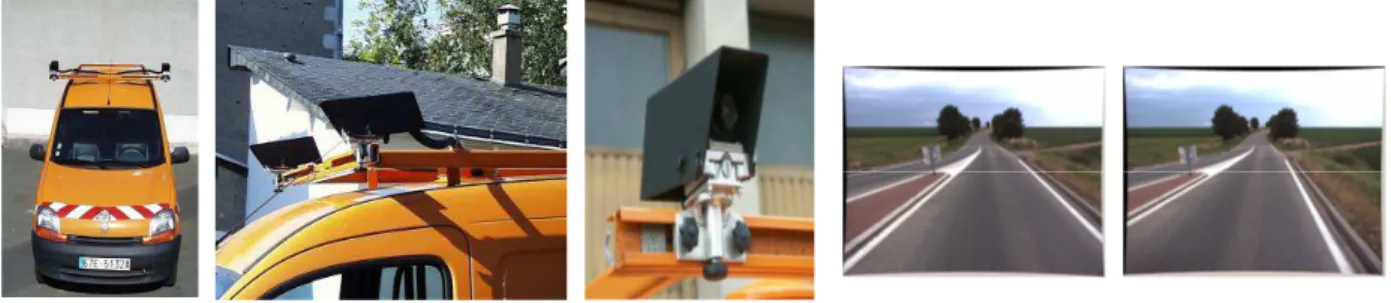
Figure 1: Experimental inspection vehicle with two digital cameras for stereovision (left 3 images, by courtesy of CECP). On the rightmost part of the figure, a stereo pair of images acquired by the vehicle is displayed.

Since road visibility evaluation by drivers is essentially a visual task, the first approach we propose exploits images taken by cameras mounted on the inspection vehicle. The use of a single camera allows only 2D measures. Two cameras are necessary to take into account the 3D shape of the road, through stereovision, during the estimation of the visibility distance. The acquisition system being reduced to two colour cameras and a computer, it is quite inexpensive. Pairs of still images (see example on Fig. 1) can be acquired every 5 meters along the path, by the vehicle at a normal speed (thus at a frame rate of around 5f/s). However, designing an accurate image processing method for estimating the 3D visibility distance remains challenging. This is due to the difficulties of 3D reconstruction from real images taken under uncontrolled illumination in the traffic.

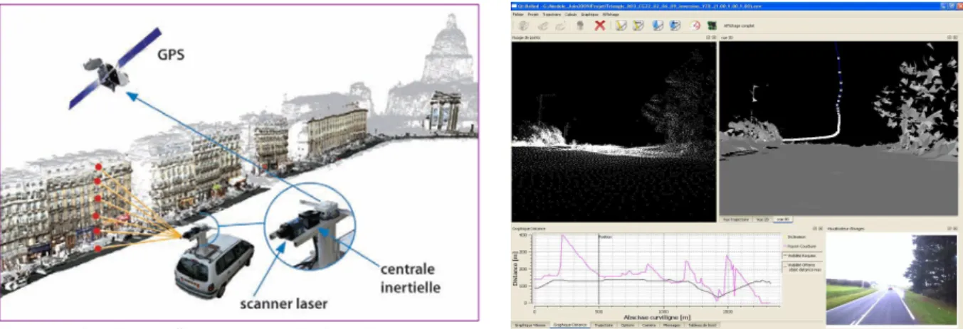
As an alternative, we also investigated the use of 3D data provided by a LIDAR terrestrial Mobile Mapping System, called LARA-3D. This prototype had been developed by the CAOR (Mines ParisTech) for several years, see (Goulette and others, 2006). Its adaptation to the creation of 3D road models for visibility computation has been initiated during the SARI-VIZIR project and developed during ANR-DIVAS project. While the vehicle moves, 3D points are sampled along the road and registered in an absolute reference system thanks to the use of INS and GPS sensors. In order to generate 3D models from points, several algorithms have been implemented, addressing particularly the need for downsizing the 3D model, and for suppressing artefacts. In order to suppress artefacts caused by the presence of vehicles, we use the position of the vehicle on the road and the approximate position of road borders, to suppress the data above the road surface. For downsizing the model, we use at first a decimation step over each scanner profile, and then a plane modelling approach based on RANSAC and region growing, followed by a Ball-Pivoting Algorithm (BPA) triangulation (Bernardini and others, 1999). This processing leads to an important reduction of the number of triangles (by a factor 10 or more). It also helps filtering artefacts, so the resulting 3D model can be fully exploited for computing visibility.

Figure 2: The LARA-3D experimental inspection vehicle of the CAOR (Mines ParisTech) is shown on the left with an example of obtained 3D point cloud and mesh on the right.

This stage provides a model of the road environment in the form of a 3D mesh, as shown in Fig. 2. Although the acquisition system is more complex and hence, more expensive than in the stereovision approach, its advantage is that 3D data is directly grabbed with high accuracy.

2.

Visibility distance using binocular stereovision

In this case, the available visibility distance is defined as the maximum distance of points belonging to the image of the road. This distance is similar to the one perceived by the driver, provided that the distance between the driver’s eye and the cameras on the roof is small. This technique was developed by LEPSiS (LCPC) during the SARI-VIZIR PREDIT project. It is estimated by a three-step processing of the pair of left and right stereo views: segmentation of the roadway on each image using colour information, registration between the edges in the road regions of the left and right images allowing to estimate a 3D model of the road surface, and estimation of the maximum 3D distance of visible points on the road.

2.1 Road segmentation

Since the roadway is of prime importance for estimating the visibility, the first step of the processing consists in classifying each pixel, in left and right images, as road or non-road. This segmentation is based on an iterative learning of the colorimetric characteristics of both the road and the non-road classes, along the image sequence. To this end, pixels in the bottom centre of each image are assumed to belong to the road class, while pixels in the top left and right regions are assumed non-road elements. These regions may be visualized in the middle image of Fig. 3. The road and non-road colour characteristics are collected in past images when the processing is running real time. However, it is better to process the sequence backwards when the algorithm can be run in batch. The reason is that it allows sampling road colours at different distances ahead of the current image. This strategy leads to improved segmentation results in the presence of lighting perturbations, shadows, variations of pavement colour. Once the road and non-road colour models are built, the image is segmented in two classes by a region growing algorithm, starting from the road (i.e. bottom centre) part of the image. Fig. 3 shows an example of segmentation result.

pixels as road and non-road pixels is shown on the right.

The non-road colour model remains stable in case of an occlusion of the non-road region, due for example to the presence of a vehicle, during a reduced number of frames. To keep a correct

road colour model, occlusions of the road region can be filtered out by removing colours which

are not usually found on the pavement. More details on this algorithm may be found in (Tarel and others, 2009).

2.2 Edge registration and road profile reconstruction

The edges found in the left and right road regions segmented in the first step differ in pose due to the change in viewpoint. This difference in pose is directly related to the shape of the road surface.

Figure 4: After matching the road edges in the left and right images, points on the road can be estimated by triangulation from the left and right viewpoints.

Assuming a polynomial parametric model of the road longitudinal profile, see Fig. 4, the second step consists in the global registration of the left and right road edges and in the estimation of the parameters of the polynomial road model. This algorithm is described in details in (Tarel and others, 2007) and is based on an iterative scheme that alternates between matching of pairs of edge pixels and the estimation of road surface parameters. The higher the number of edges (even those due to dust on the road may be useful), the better the registration. Of course, occulted parts of the road can not be correctly reconstructed. However, situations where a vehicle completely hides the road were rarely observed in practice.

Left image

Right image Road surface

2.3 Road visibility distance estimation

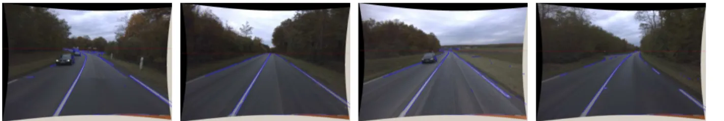
Once the 3D surface of the road has been estimated from the second step of the processing, the maximum distance at which edges of the left and right images can be registered is computed. Finally, the road model is used to convert this distance to a metric estimate of the highway visibility distance. Examples of results are shown in Fig. 5, where the red line corresponds to the visibility height in each image. As explained in details in (Bigorgne and others, 2008), the standard deviation of the estimator is also computed, in order to qualify this estimated visibility distance.

Figure 5: The blue edges are those edges of the right image that were registered on the left image, which is displayed. These images are extracted from a sequence of 400 images.

3.

Visibility distance from a 3D model of the road and its surroundings

In this approach, we exploit both the 3D triangulated data provided by the LIDAR system and the trajectory recorded by GPS/INS integration to estimate visibility distances.

3.1 Estimating the visibility distance from a 3D model

The definition of the available visibility distance we use in this approach is purely geometric and does not involve any photometric or meteorological consideration. It involves a target and an observer. The target may either be placed at a fixed distance from the observation point, to assess the availability of a specific distance, or it may be moved away from the observation point until it becomes invisible, to estimate the maximum visibility distance.

Conventional values can be found in the road design literature, see (SETRA, 2000) and (SETRA, 1994), for both the location of the observer and the geometry and position of the target. Both the viewpoint and the target are centered on the road lane axis. Typically, the viewpoint is located one meter high, which roughly corresponds to a mean driver's eye position. The conventional target is a pair of points that model a vehicle's tail lights. For visibility distance computation, we request a line-of-sight connection between the tail lights and the driver’s eyes. Ray-tracing algorithms are well-suited for this task. We also found it realistic to consider a parallelepiped (1.5×4×1.3 m) to model a vehicle. We found that a good rule of thumb was to consider the target as visible if 5% of its surface is visible. The threshold was set experimentally, in such a way that the results of the test would be comparable to the ones obtained when using the conventional target.

3.2 Qt-Ballad: a tool for visibility estimation

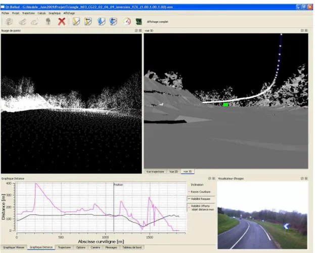
ERA 27 (LCPC) developed a specific software application, called Qt-Ballad (see Fig. 6) during the SARI-VIZIR PREDIT project. It allows to walk through the 3D model (which can be visualized as a point cloud or a surface mesh). The trajectory of the inspection vehicle on the

Figure 6: interface of the Qt-Ballad software. The top-left panel displays the original point cloud. The top-right panel shows the triangulated model (in grey), the trajectory of the LIDAR system (in blue) and a parallelepiped target placed 100 m ahead of the observation point (in green). At the bottom right, an image of the scene is displayed. Finally, the bottom-left panel displays the required visibility (black) and the estimated available visibility (magenta) vs. the curvilinear abscissa. The vertical line shows the current position. The curves show that the available visibility is not sufficient in this situation.

Qt-Ballad implements both required and available visibility distance computation. For the point-wise, conventional target, we use a software ray-tracing algorithm. When the volumetric target is used, we exploit the Graphical Processing Unit's capabilities. More specifically, the target is first drawn in the graphical memory, then the scene is rendered using Z-buffering and finally, an

occlusion-query request (which is standard in up-to-date OpenGL implementations) provides the

percentage of visible target surface. The visibility distance can be computed at every point of the trajectory (i.e. every 1 meter) or with a fixed step (typically, 5 or 10 meters) to speed up computations.

Two different ways of computing the visibility are implemented. In the first case, a fixed distance is maintained between the observation point and the target. The output is a binary

function which indicates at every position whether the prescribed distance is available or not. In the second case, for every position of the observation point, the target is moved away as long as it is visible and the maximum available visibility distance is recorded.

4.

Discussion

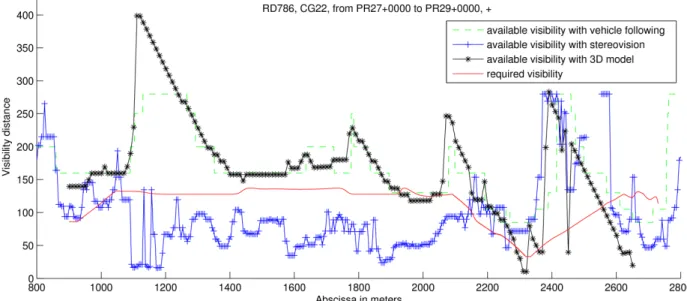
Within the SARI-VIZIR PREDIT project, see (Tarel and others, 2008), different kinds of road section have been selected to perform a comparative study. Three approaches were tested: using stereovision, using a 3D model and using vehicle following. The last method, called VISULINE, see (Kerdudo and others, 2008), is used as a reference. It consists of two vehicles, connected by radio in order to maintain a fixed distance. An operator, in the following vehicle, checks visually whether the leader vehicle is visible or not. To estimate the maximum visibility distance, the vehicle-following system had to be run for several intervals: 50, 65, 85, 105, 130, 160, 200, 250 and 280 meters. The result is shown for a 2 km road section of RD768, CG22, as a green discontinuous curve, see Fig. 7. On the same figure, the required visibility distance computed from the road characteristics is shown as a red, continuous curve. Estimated available visibility obtained using stereovision is displayed as a blue curve with pluses, and the black curve with stars shows the results of the approach based on 3D modelling.

Figure 7: Comparison on the same 2 km road section (RD786, CG22), of the estimates of the available visibility distance using 3 techniques: vehicle following, stereovision, 3D model. The required visibility computed from the road geometry is also displayed. When the available visibility is lower that the required one (e.g. at abscissa 2000 m), a lack of visibility is detected.

The results show that the stereovision approach under-estimates the visibility distance over most of the length of the section. A careful examination of the results has shown that the algorithm is very sensitive to the presence of vehicles in the road scene. Moreover, the long range road/non-road classification becomes more difficult when colors are flatter, which occurs under certain weather conditions or during the winter. The results of the 3D-based method are in good accordance with those of the reference method. However, we recall that the vehicle-following

alternative to LIDAR sensors and we plan to investigate this in the near future.

5.

Acknowledgements

The authors are thankful to the French PREDIT SARI-VIZIR and ANR-DIVAS projects for funding. The VISULINE data was provided by the LRPC St Brieuc (ERA 33 LCPC).

6.

References

1. SETRA (2000), ‘ICTAAL : Instruction sur les Conditions Techniques d’Aménagement des Autoroutes de Liaison’, circulaire du 12/12/2000.

2. SETRA (1994), ‘ARP : Aménagement de Routes Principales (sauf les autoroutes et routes express à deux chaussées)’, 08/1994. Chapter 4 and Appendix 3.

3. Goulette F., Nashashibi F., Abuhadrous I., Ammoun S. & Laurgeau C. (2006) , ‘An Integrated On-Board Laser Range Sensing System for On-The-Way City and Road Modelling’. Int. Archives of the Photogrammetry, Remote Sensing and Spatial Information

Sciences, Vol 34, Part A.

4. Bernardini F., Mittleman J., Rushmeier H. & Silva C. (1999), ‘The Ball Pivoting Algorithm for surface reconstruction’, IEEE Trans. On Visual and Computer Graphics, vol. 5, no. 4, pp. 349-359.

5. Tarel J.-P. & Bigorgne E. (2009), ‘Long-Range Road Detection for Off-line Scene Analysis’,

Proceedings of the IEEE Intelligent Vehicle Symposium (IV'09), China, pp. 15-20.

6. Tarel J.-P., Ieng S.-S. & Charbonnier P. (2007). ‘Accurate and Robust Image Alignment for Road Profile Reconstruction’, Proceedings of the International Conference on Image

Processing (ICIP'07), USA, pp. 365-368.

7. Bigorgne E., Charbonnier P. & Tarel J.-P. (2008), ‘Méthodes de mesure de la visibilité géométrique’, SARI-VIZIR PREDIT project, action 1.2 – Livrable n° 1.2.4.

8. Tarel J.-P., Charbonnier P., Désiré L., Bill D. & Goulette F. (2009), ‘Evaluation comparative des méthodes de mesure de la distance de visibilité géométrique’, SARI-VIZIR PREDIT

project, action 3.1 – Livrable n° 3.1.2.

9. Kerdudo K., Le Mestre V., Charbonnier P., Tarel J.P. & Le Potier G., ‘La visibilité géométrique : quels outils de diagnostic ?’ Revue Générale des Routes et Autoroutes, n°865, march 2008.